Article

Automatic Recognition of Vertical-Line Pulse Train from China Seismo-Electromagnetic Satellite Based on Unsupervised Clustering

1
Institute of Disaster Prevention, Sanhe 065421, China
2
Microelectronics and Optoelectronics Technology Key Laboratory of Hunan Higher Education, School of Physics and Electronic Electrical Engineering, Xiangnan University, Chenzhou 423000, China
3
Hunan Engineering Research Center of Advanced Embedded Computing and Intelligent Medical Systems, Chenzhou 423000, China
4
National Institute of Natural Hazards, Ministry of Emergency Management of China, Beijing 100085, China
5
National Space Science Center, Chinese Academy of Sciences, Beijing 100085, China
6
Faculty of Arts, Hebei University of Economics and Business, Shijiazhuang 050061, China
*
Author to whom correspondence should be addressed.
Atmosphere 2023, 14(8), 1296; https://doi.org/10.3390/atmos14081296
Submission received: 24 July 2023 / Revised: 11 August 2023 / Accepted: 14 August 2023 / Published: 16 August 2023

Abstract

:
Pulse signals refer to electromagnetic waveforms with short duration and high peak energy in the time domain. Spatial electromagnetic pulse interference signals can be caused by various factors such as lightning, arc discharge, solar disturbances, and electromagnetic disturbances in space. Pulse disturbance signals appear as instantaneous, high-energy vertical-line pulse trains (VLPTs) on the spectrogram. This paper uses computer vision techniques and unsupervised clustering algorithms to process and analyze VLPT on very-low-frequency (VLF) waveform spectrograms collected by the China Seismo-Electromagnetic Satellite (CSES) electric field detector. First, the waveform data are transformed into time–frequency spectrograms with a duration of 8 s using the short-time Fourier transform. Then, the spectrograms are subjected to grayscale transformation, vertical line feature extraction, and binarization preprocessing. In the third step, the preprocessed data are dimensionally reduced and fed into an unsupervised K-means++ clustering model to achieve automatic recognition and labeling of VLPTs. By recognizing and studying VLPT, not only can interference be recognized, but the temporal and spatial locations of these interferences can also be determined. This lays the foundation for identifying VLPT sources and gaining deeper insights into the generation, propagation, and characteristics of electromagnetic radiation.

1. Introduction

Since the mid-20th century, with the development of space technology, satellites have been used as observation platforms to acquire electromagnetic wave data from Earth and the universe. They have been widely applied in fields such as meteorology, geophysics, environmental science, and astronomy [1,2,3,4,5]. Satellite observations provide global-scale electromagnetic wave data, including a large number of electromagnetic disturbances such as lightning, solar magnetic storms, and ionospheric disturbances [6,7,8,9]. By identifying and studying these disturbances, we can not only monitor and predict space weather phenomena and predict earthquakes but also provide information on ionospheric and atmospheric activities for sectors such as aviation, aerospace, communications, and navigation. In addition, it helps to gain a deeper understanding of the generation, propagation, and characteristics of electromagnetic radiation.
Electromagnetic pulse interference signals refer to electromagnetic waveforms with short time duration and high peak energy. Spatial electromagnetic pulse interference signals can be caused by various factors, such as lightning, arc discharge, solar disturbances, and spatial electromagnetic wave disturbances [10,11,12]. A spectrogram is a tool used to describe the temporal and spectral variations of a signal. By applying time–frequency analysis techniques (such as the short-time Fourier transform), we can visualize the temporal and frequency domain information of the signal [13,14,15,16]. Pulse disturbance signals appear as instantaneous, high-energy vertical lines on the spectrogram [17]. Pulse signals typically have a wide frequency spectrum, so vertical lines on the spectrogram may cover multiple frequencies. These vertical-line pulse trains (VLPTs) indicate the pulse occurrence time and frequency distribution characteristics.
At present, the identification of different types of spatial electromagnetic waves on spectrograms mainly focuses on two aspects: constant frequency electromagnetic wave identification and L-shape whistler wave identification. However, there is currently limited research and application for the identification of other types of electromagnetic waves. Constant frequency electromagnetic wave identification refers to the classification and identification of electromagnetic waves within specific frequency ranges, which appear as horizontal lines on the spectrogram, such as wireless communication frequency bands. By using computer techniques to identify horizontal lines on the spectrogram, different types of constant-frequency electromagnetic wave sources can be distinguished, enabling identification and classification [18,19,20]. L-shaped whistler waves, on the other hand, refer to a special-shaped electromagnetic wave signal with unique spectral characteristics and temporal patterns. L-shape whistler waves can be manually labeled with an L-shape tag and be automatically identified using deep learning methods [21]. In addition, article [22] introduces the method of using convolutional neural networks (ConvNet) for automated ULF (ultra-low frequency) wave classification in swarm time series. However, for other types of electromagnetic waves, such as random frequencies or irregular signal spectra, there are currently no definite methods or research findings for their identification.
During its five years of operation, the CSES satellite has accumulated a significant amount of data resources, which contain rich and complex information on electromagnetic wave disturbances in space. In order to delve into the inherent value of these data, there is an urgent need to employ advanced batch processing techniques of big data to extract hidden electromagnetic disturbance information from it.
This paper uses computer vision techniques and unsupervised clustering algorithms to automatically recognize VLPTs on spectrogram of VLF waveform data collected by the CSES electric field detector. By studying spectral distribution and duration, automatic recognition of VLPT is realized. This study proposes new methods and approaches for automatically recognizing VLPT and locating disturbance sources, providing technical support for electromagnetic radiation research and related fields of application.

2. Data Collection

The China Seismo-Electromagnetic Satellite (CSES) was successfully launched on 2 February 2018. It is China’s first dedicated space science satellite for studying seismic electromagnetics [23,24,25,26,27]. The CSES satellite is designed to investigate electromagnetic phenomena and related physical mechanisms in the field of geophysics before and after seismic events. CSES is equipped with a series of scientific instruments, including a fluxgate magnetometer (FGM), electric field detector (EFD), plasma analyzer package (PAP), Langmuir probe (LP), low-energy charged particle analyzer (LECPA), high-energy particle detector (HEPD), seismo-electromagnetic (SEM) field detector, etc. [28,29,30,31]. These instruments work together to study various phenomena in space, including electromagnetic waves, plasma dynamics, magnetic field variations, and their interactions with seismic activities on Earth. Since the launch of the CSES satellite, many studies and experiments have been carried out, including space weather research, ionosphere and electromagnetic wave research, earthquake prediction research, and Earth observation and environmental research [32,33,34,35,36,37].
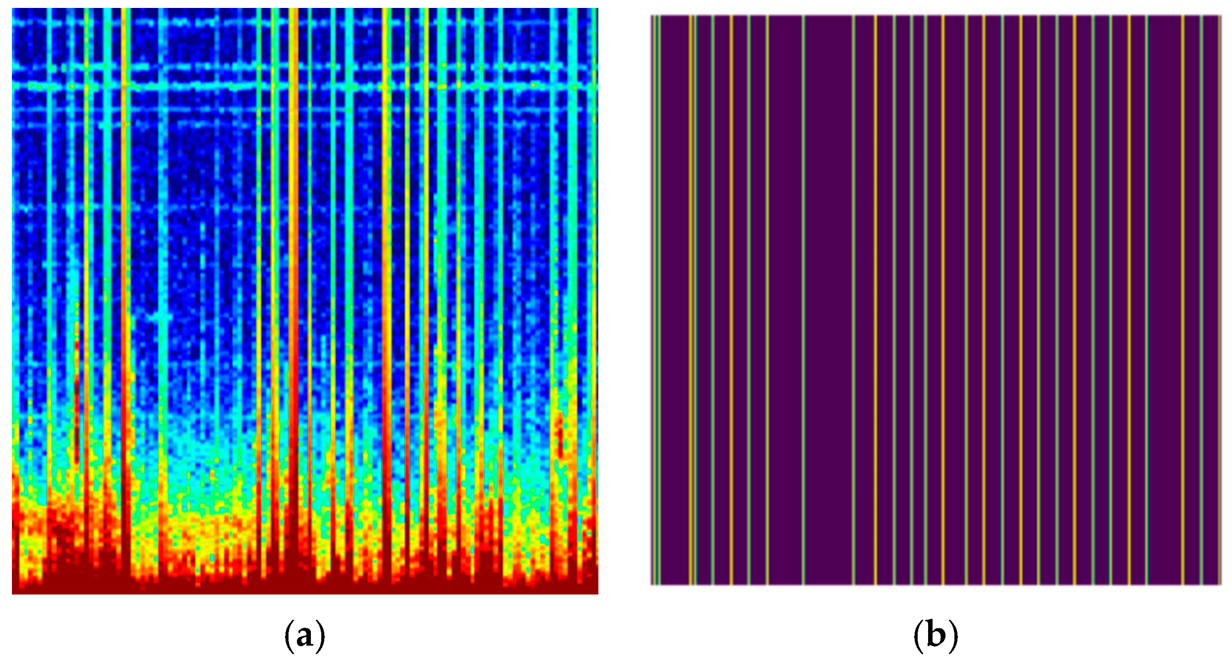
In this experiment, we processed VLF waveform data collected by the CSES EFD over the period 2019–2020. By performing short-time Fourier transform, we converted the waveform data into a time–frequency spectrogram, as shown in Figure 1. The spectrogram illustrates the temporal and frequency variations of an 8 s signal. In the spectrogram, the x-axis represents time with a length of 8 s, the y-axis represents frequency, and the color bar represents signal intensity. The time–frequency spectrogram obtained by short-time Fourier transform provides an intuitive way to simultaneously display the time domain and frequency domain information of the signal. By observing changes in the spectrogram, we can analyze the temporal and frequency characteristics of the signal’s evolution, thus gaining deeper insights into the behavior of very-low-frequency waveforms.

3. Automatic Recognition Algorithm of VLPT

Clustering analysis, as an unsupervised learning method, involves grouping or categorizing samples according to their measured similarity. This paper aims to use unsupervised clustering learning methods to automatically recognize VLPTs with varying energies, as shown by the different energy vertical lines in Figure 1b. The algorithm flowchart for VLPT recognition is shown in Figure 2.
  • Grayscale: The color image is converted into a grayscale image.
  • Edge feature enhancement: Edge enhancement algorithms are applied to enhance the edge features of vertical lines in the grayscale image.
  • Binarization: The enhanced grayscale image is converted into a binary image, where each pixel has only two values, typically black and white.
  • Data dimensionality reduction: Each pixel column is treated as a recognition sample.
  • Unsupervised clustering: The K-means++ clustering algorithm is used to cluster pixel columns into different clusters or categories based on their similarity.
  • Automatic marking: The identified lines are automatically marked, facilitating further observation and analysis.

3.1. Grayscale

Grayscale conversion is the process of transforming a color image into a grayscale image, where the value of each pixel is represented in a grayscale color space instead of the RGB (redgreenblue) color space. This conversion is performed to reduce computational complexity and storage requirements and facilitate further image processing tasks. There are various methods available for grayscale conversion. In an RGB color image, each pixel consists of numerical values for the red (R), green (G), and blue (B) channels. The blue channel refers to the numerical value of the blue component for each pixel in the image. In this paper, the blue channel is used to achieve grayscale conversion [19].
  G r a y ( x , y )   =   R G B B ( x , y )
where, RGB refers to the original color spectrogram, (x, y) represents the coordinates of a pixel on the image, and it corresponds to the blue (B) channel. Figure 1b shows an original spectrogram to be recognized, and Figure 3 shows the resulting spectrogram after the grayscale conversion process.

3.2. Vertical Edge Features Enhancement

Edge detection helps to capture the contour of edges between objects and the background in an image. To enhance the features of the vertical line edge in the image, a vertical edge detection filter can be applied. In order to improve computation speed, this paper uses a 1 × 3 convolution kernel, as shown in Equation (2).
K e r n e l = [ [ 1 , 0 , 1 ] ]
By applying the convolution Kernel to the convolution operation expression in Equation (3), vertical edge feature enhancement is achieved.
O u t p u t ( x , y ) = s t K e r n e l ( s , t ) I n p u t ( x s , y t )
where I n p u t represents the input image, (x, y) represents the pixel coordinates, (s, t) represents the position of the convolution kernel elements, and o u t p u t represents the output image. Step 1 is used, and pixel copy edge padding is used. By applying the vertical edge enhancement filter to the grayscale image in Figure 3, the resulting image is shown in Figure 4.

3.3. Binarization

Image binarization is the process of setting pixel values in an image to either 0 or 255, resulting in a clear black and white effect throughout the entire image. By binarizing the image, it reduces the dimensionality of the image data while eliminating interference from factors such as noise, allowing the contours of the regions of interest to be clearly displayed. This method of processing provides clearer and more effective basic data for subsequent image processing and analysis. The binarization formula is expression in Equation (4).
d s t ( x , y ) = { m a x V a l if   s r c ( x , y ) > t h r e s h 0 otherwise
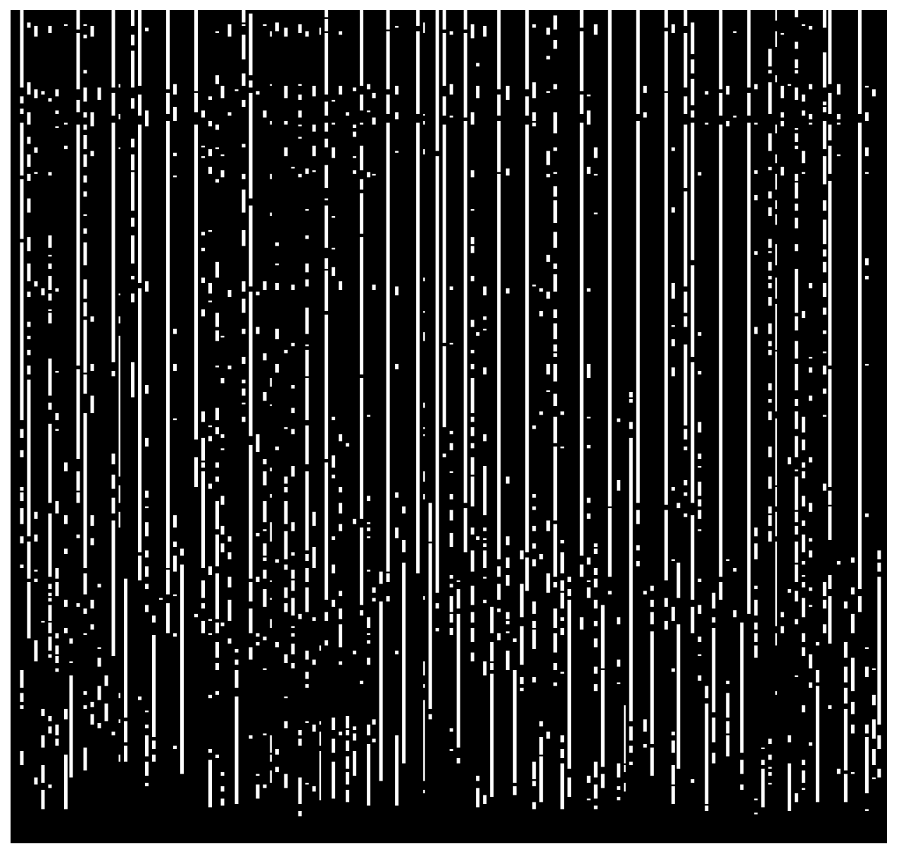
Here dst is the output image, maxVal is the maximum value set (in this experiment, it is set to 255), src is the input image, thresh is the fixed threshold value set (in this experiment, thresh is set to 35). Pixels with values greater than 35 are set to 255, while pixels with values less than 35 are set to 0. (x, y) represents the coordinates of pixels. The results of binarization are shown in Figure 5.

3.4. Data Dimensionality Reduction

The purpose of this experiment is to identify vertical lines. Clustering algorithms typically group data samples based on some similarity measure to maximize intra-cluster similarity and minimize inter-cluster similarity. In order to extract the features of these vertical lines and understand the data, we perform dimensionality reduction on the image before clustering. We use the column pixels of the image as the basic processing unit for this dimensionality reduction.
Assuming there is an m × n binary image corresponding to a two-dimensional data matrix, where each column represents a feature, resulting in a total of n features.

3.5. Unsupervised Clustering

Unsupervised clustering is a machine learning task that aims to partition data samples into similar groups or clusters without requiring prior knowledge of labels or class information. Unlike supervised learning, where models rely on external guidance, unsupervised learning performs clustering by discovering the inherent structure and similarities within the data [38].
In unsupervised clustering tasks, algorithms automatically identify and learn similarities between data samples. They assign similar data points to the same cluster while assigning dissimilar data points to different clusters. Unsupervised clustering finds wide applications in many fields and domains, including data mining, image analysis, text mining, recommendation systems, and more. Unsupervised clustering models belong to a class of models in unsupervised learning used to discover underlying categories or cluster structures in unlabeled datasets. Here are several common clustering models: K-means clustering [39], hierarchical clustering [40], density-based spatial clustering of applications with noise (DBSCAN) [41], spectral clustering (SC) [42], etc.
The computational complexity of K-means clustering is relatively low, and it is computationally efficient. The trained model can be pre-trained and used to predict new samples. Spectral clustering is a clustering algorithm based on graph theory. It constructs a graph using similarity between data samples and performs dimensionality reduction and clustering based on graph features. Spectral clustering, in contrast to traditional clustering algorithms such as K-means, does not generate a model that can be used to predict new samples.
Therefore, in this experiment, combining the idea of dimensionality reduction with spectral clustering, we use the K-means model to train and predict the reduced matrix. First, we perform dimensionality reduction and clustering on feature vectors by considering them as column vectors. Then, we preprocess and reduce a set of clear VLPT spectrograms, as shown in Figure 1b, which serve as training samples for the K-means model. We use the trained model to predict new samples.
Unsupervised clustering model K-means clustering: Using selected cluster centers as initial centers, run the allocation and update steps of the K-means algorithm iteratively until the convergence condition is met. K-means++ is an improved version of the K-means algorithm that enhances the selection of initial cluster centers to improve the accuracy and stability of clustering results. Here are the steps of the K-means algorithm:
  • Randomly select a data point as the first cluster center.
  • For each data point, calculate the squared distance to the cluster centers already selected and use it as a weight.
  • Based on distance weights, select the next cluster center with a higher probability. For each data point, normalize the weights, and then select the next cluster center probabilistically.
  • Repeat steps 2 and 3 until K cluster centers are selected.

3.6. The Predetermined Number of Clusters, K

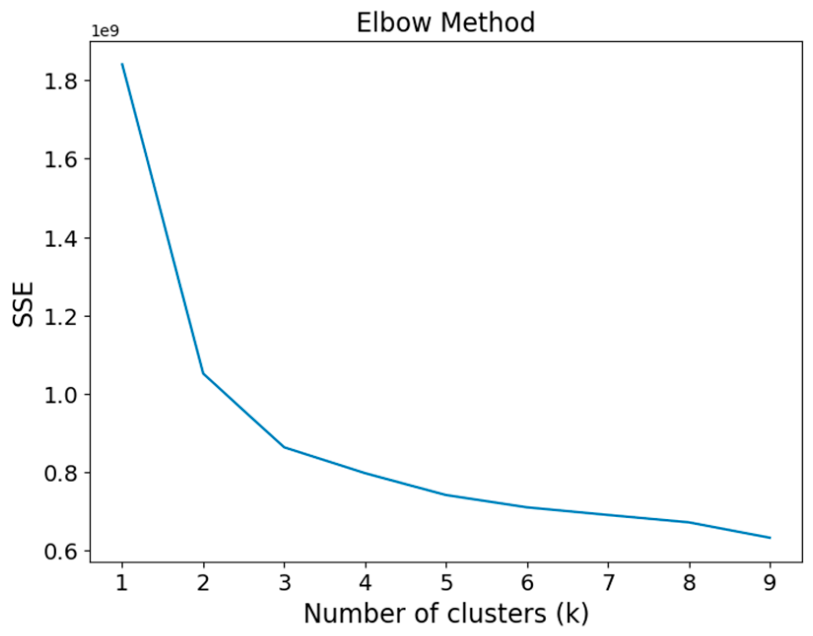
In the K-means algorithm, K refers to the number of clusters to be formed, also known as the predetermined number of clusters. The appropriate value of K is crucial for the effectiveness of the K-means algorithm and the quality of clustering results. A common method of determining the value of K is experimentation and adjustment based on data characteristics and domain knowledge. There are also quantitative methods such as the elbow method, silhouette coefficient, and within-cluster sum of squares (WCSS) to assist in this determination. The elbow method involves plotting the curve of the sum of squared errors (SSE) of clusters under different K values and selecting the K value at the “elbow” point where the curve begins to level off. The silhouette coefficient, on the other hand, evaluates the compactness and separation of clustering results based on similarity and dissimilarity among samples as shown as Figure 6.
After dimensionality reduction, the data about Figure 5 is fed into the K-means++ model for training. The curve of the sum of squared errors (SSE) at different values of K is plotted, and the value of K is chosen based on the location where the curve exhibits an elbow bend. It is observed that the optimal number of clusters corresponds to the inflection point, which in this case is K = 2. This result is further supported by calculating the silhouette coefficient, also yielding K = 2. Furthermore, considering the practical requirements of the experiment to divide the data into two categories: straight lines and non-straight lines, K = 2 is appropriate based on the actual application.
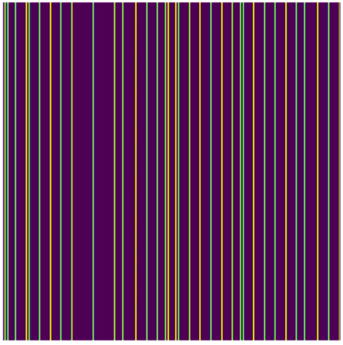
Therefore, in this paper, we set K = 2, representing two categories: straight lines and non-straight lines. The clustering operation is performed on each column as the clustering element. After clustering, each row is assigned a label representing either a straight line or a non-straight line. The visualization of the labeled straight lines after training the model is shown in Figure 7.

3.7. Automatic Labeling of Recognition Results

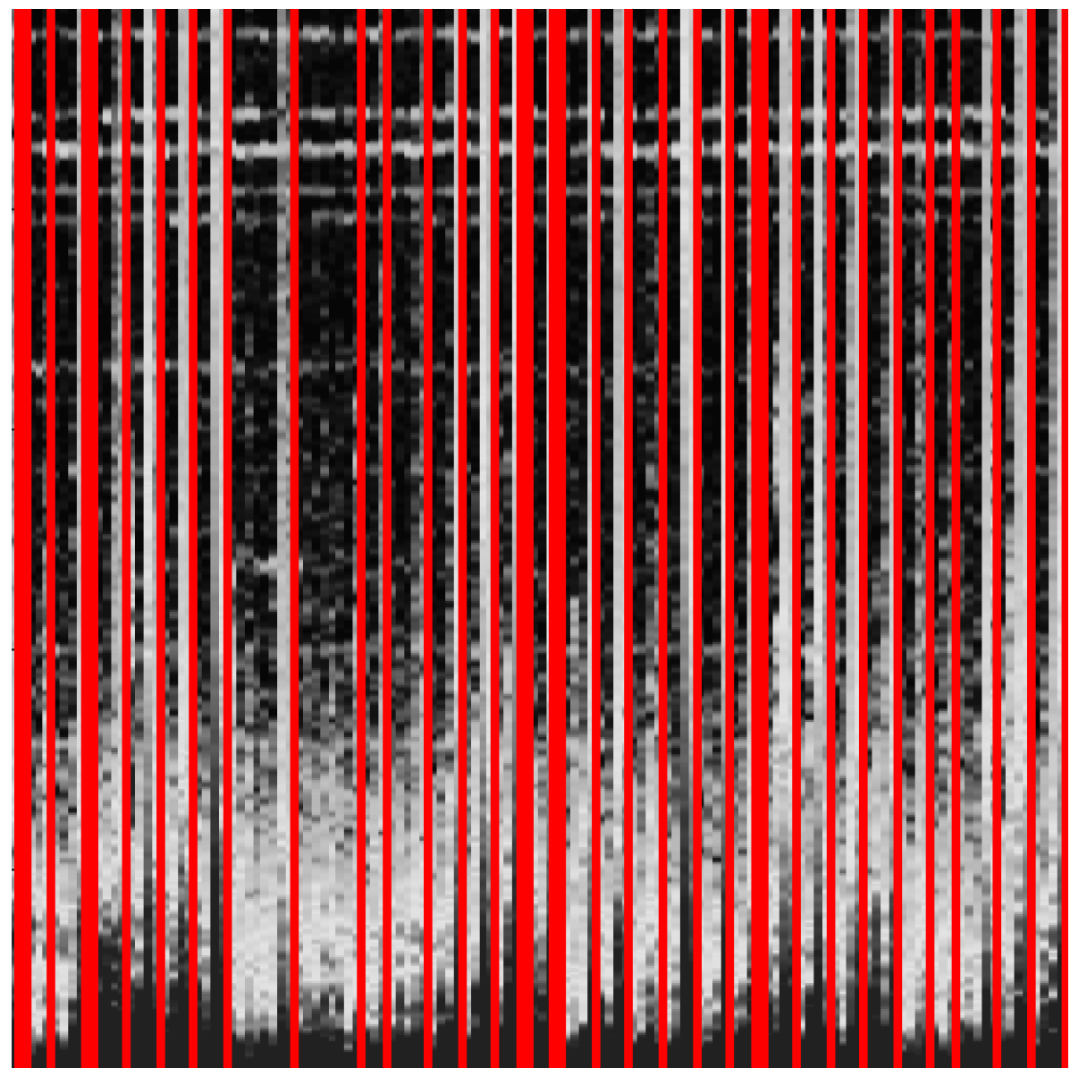
After clustering, column pixels are classified into straight-line and non-straight-line classes. To facilitate further visual observation and analysis, the pixel columns identified are marked with red lines. Due to variations in the energy and color of VLPTs in the original image, in order to observe the clustering results clearly, red lines are used for marking on the grayscale image. Figure 8 shows an example of the marked results.

4. Experimental Setup and Results Analysis

4.1. Experimental Environment

For this experiment, MATLAB 2020 was used to generate spectrograms. Python 3.7 was used with the OpenCV and Scikit-learn libraries for feature extraction and clustering algorithms. This implementation enabled automatic recognition of electromagnetic pulse sequence signals.

4.2. Experimental Data

The experimental data used in this study were obtained from VLF waveform data collected by the CSES EFD from 2019 to 2020. They include complete revisited track cycle waveform data and a random set of waveform data. A total of 8558 spectrograms were produced.

4.3. Experimental Method

4.3.1. Data Preprocessing

For each track dataset, multiple spectrograms with a duration of 8 s were generated. The following preprocessing steps were applied to each spectrogram: grayscale conversion, edge feature enhancement, and binarization. Taking a spectrogram (denoted Figure 9a) with fewer vertical lines as an example, the results of each preprocessing step are shown in Figure 9b–d.

4.3.2. Model Training

A K-means++ model is established with K = 2. A spectrogram with clear and abundant vertical lines, such as shown in Figure 10a, is selected. After the aforementioned preprocessing steps, each column of pixels is treated as a sample vector and undergoes dimensionality reduction. These vectors are then fed into the model for training. By accessing the label attribute of the K-means++ model, the clustering labels of each column vector sample can be obtained. The labels representing the vertical lines are visualized in Figure 10b.

4.3.3. Prediction

After training the K-means++ model and obtaining the clustering labels for the training samples, we can now use this trained model to make predictions on new or unseen samples.
To predict on new samples, we apply the same preprocessing steps as before to obtain the binary image data. We then pass these data to the model’s prediction method. The model will assign each new sample a clustering label based on the similarity to the existing clusters.
For example, in the case of the 2D image shown in Figure 10d, after performing dimensionality reduction and passing it to the trained model, we obtain the predicted clustering labels. The visualization of the labels representing the vertical lines in the new samples is displayed in Figure 11a. Additionally, the predicted results can be observed in Figure 11b.

4.4. Comparative Analysis of Results from Different Experimental Methods and Conclusions

In this experiment, we tested different line recognition algorithms and clustering algorithms, including Hough line detection, hierarchical clustering, DBScan clustering, spectral clustering, and improved K-means++ clustering. The results of each algorithm’s line recognition are shown in Figure 12.
According to the experimental results, we can observe the following: the Hough line detection method detects both horizontal and vertical lines as line segments; the hierarchical clustering model recognizes many false detections; the DBScan clustering model misses many line detections; spectral clustering and the improved K-means++ approach used in this study have similar identification performance. However, K-means++ demonstrates higher time efficiency. The statistical analysis of spectral clustering and K-means++ clustering is shown in Table 1.
In terms of time efficiency, K-means++ outperforms spectral clustering because K-means++ can be pre-trained, eliminating the need for training the model from scratch each time. This makes K-means++ more time-efficient than spectral clustering. Therefore, in this experiment, we combined the dimensionality reduction concept of spectral clustering with the high time efficiency of K-means++. This algorithm not only achieves high recognition accuracy, but also demonstrates high efficiency.

4.5. VLPTs Recognition

According to the method described above for recognizing straight lines on the spectrogram, Figure 13 shows the results of vertical line recognition in different spectrograms.
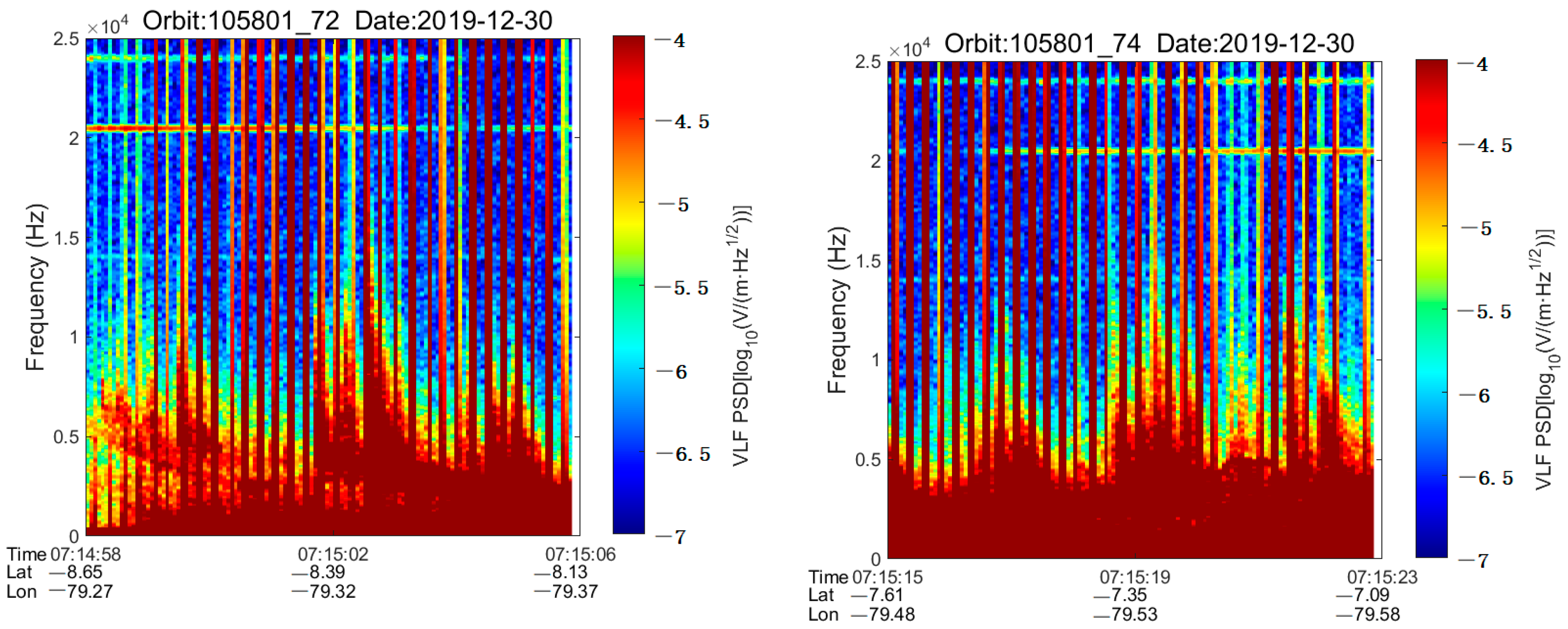
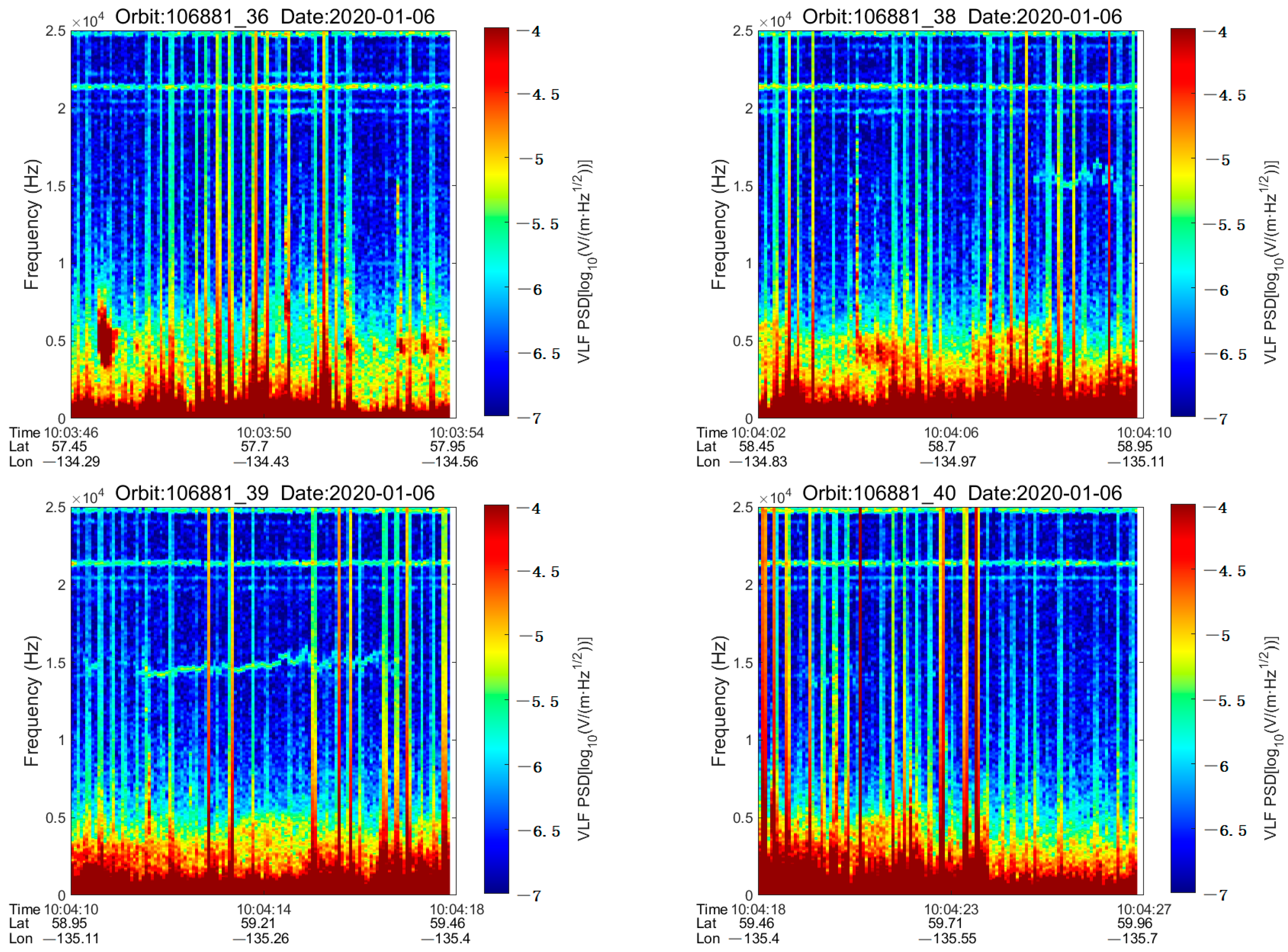
By comparing Figure 13, we can observe that the greater the number of recognized lines, the greater the disturbance. To optimize the recognition process, we introduced a variable linesnum, which represents the number of column vectors representing row clusters detected in an 8 s spectrogram. Analyzing linesnum, we found that spectrograms with linesnum > 60 usually indicate significant perturbations. We recorded the spectrograms with linesnum > 60. Using this method, we can not only recognize prominent VLPTs that indicate significant perturbations but also determine their spatial and temporal perturbations. The following two sets of spectrograms are examples of VLPTs found in a massive dataset, as shown as Figure 14 and Figure 15, all of which satisfy linesnum > 60. This method effectively filters out high-energy VLPTs from vast amounts of data and obtains their spatial and temporal information.

5. Discussion

There can be multiple causes for VLPT generation, and here are some potential sources: Lightning is the result of charge separation and discharge in the atmosphere, which can generate intense pulsed electromagnetic radiation [10,11,12]. Solar activities, such as solar flares and solar bursts, can also cause pulsed electromagnetic wave radiation, and the energy released from these solar activities can trigger electromagnetic pulses in nearby space on Earth. The ionosphere, which is a layer of ionized gas in the Earth’s atmosphere, plays an important role in the propagation and reflection of electromagnetic waves. Disturbances in the ionosphere, such as ionospheric irregularities, shear layers, and fluctuations, can cause pulsed electromagnetic wave radiation. Conforming propagation is a phenomenon in the propagation of electromagnetic waves, where pulsed signals may be formed due to interference from different paths after the reflection of electromagnetic waves in the atmosphere. These are just some of the possible reasons for VLPT generation, and the actual situation may be more complex and require specific analysis based on the data and scenario.
There have been many methods proposed by previous researchers for the identification of pulse signals. One approach is based on the extraction of timedomain features, such as pulse width, peak value, and pulse shape, for signal classification and recognition [43,44]. Another approach is through frequencydomain feature extraction: the pulse signal is transformed using Fourier transform or wavelet transform, and features such as spectral distribution and frequency components are extracted for signal classification and recognition [45,46]. The third method utilizes morphological transformations to process the pulse signal and extract morphological features, such as skeleton, convex hull, and valleys, for signal classification and recognition [47,48]. The fourth method involves using machine learning algorithms for pulse signal classification, such as support vector machines, artificial neural networks, and decision trees [49,50]. Although these are some common methods for pulse signal extraction, and in practical applications, specific tasks and data characteristics may require the selection of appropriate methods. For example, reference [43] proposed a pulse signal analysis and recognition method based on multiscale morphological component analysis. It applies multiscale morphological transformations to the original signal, extracts specific features from the transformed results, and then utilizes a classifier for signal recognition. The success of this method is sensitive to parameter selection, as the choice of parameters can significantly impact the final recognition results. Reference [51] presented a feature extraction framework for underwater pulse signals based on morphology and wavelet packet transform, specifically for the field of ocean and underwater signal processing. This method has the capability of multiscale analysis and powerful spectral analysis, but its applicability may be limited to specific types of underwater pulse signals or specific application scenarios. Reference [52] used a Gaussian distribution-based electromagnetic pulse model and estimated parameters such as shape, amplitude, and duration of the pulse to describe the characteristics of ultra-wideband electromagnetic pulses. The methods for estimating these parameters are detailed in the article, and their effectiveness is validated through experimental results. However, this method is only applicable to Gaussian-distribution-based electromagnetic pulses and may not be suitable for other pulse distributions.
This paper employs computer vision techniques and unsupervised clustering algorithms on the spectrogram obtained through the Fourier transform to realize automatic recognition of VLPT. The vertical line recognition algorithm proposed in the paper is applicable to the recognition of vertical lines on any type of spectrogram. And this method not only identifies VLPT but also discovers their spatiotemporal locations.
Although this method allows us to find the spatiotemporal positions of these significant electromagnetic disturbances, further confirmation is needed to determine the sources of these disturbances. In addition, research is needed on the physical characteristics, propagation mechanisms, and potential effects of electromagnetic pulse radiation on electronic systems.

6. Conclusions

This study used computer vision techniques and unsupervised clustering algorithms to process and analyze VLF waveform data collected by the CSES satellite’s EFD. First, the waveform data were transformed into an 8 s spectrogram using the short-time Fourier transform. The spectrogram was then processed by grayscale conversion, vertical edge feature enhancement, and binarization. The preprocessed data were columnwise dimensionality reduced and fed into an unsupervised K-means++ clustering model for training and prediction, enabling the identification of vertical lines on the spectrogram. Any vertical line on the spectrogram identified as exceeding 60 lines is considered the recognized VLPT result. It realized automatic recognition and labeling of VLPT disturbances as well as localization of the spatiotemporal positions of pulse signals.
Pulse interference signals can potentially disrupt satellite communication or observation tasks. By promptly identifying and locating the source of interference and implementing appropriate interventions, the normal operation of satellites can be ensured. Additionally, in applications such as satellite communication and radar systems, analyzing the spectrogram of pulse signals allows for the study of signal propagation effects in the atmosphere, ionosphere, or other media. This analysis further enables the optimization of signal transmission and reception performance.
In conclusion, the results of this study provide new methods and approaches for automatic recognition and localization of VLPTs. This provides the basis for electromagnetic wave disturbance monitoring, space weather research, earthquake prediction, and related applications. It will contribute to enhancing our understanding of environmental changes and natural phenomena and provide more reliable data support for the development and application of relevant industries. Future work will focus on the following areas:
  • Further study of spectral distribution, duration, power characteristics, etc., of interference signals to enhance the ability to identify different types of interference sources. By establishing a library of interference signals, modeling and classifying signals generated by different interference sources can improve the accuracy of identification.
  • Research and apply more efficient data preprocessing and noise reduction techniques to improve the quality of VLF waveform data. For example, filtering methods are used to optimize signal to noise ratio.

Author Contributions

Conceptualization, methodology, writing—original draft, and writing—review and editing, Y.H.; methodology, Y.L. and J.Y.; funding acquisition, Y.L. and Y.L.; data curation, J.H.; supervision, X.S.; editing, L.M. and Y.Z.; investigation and resources, Z.L., Y.W. and X.C. All authors have read and agreed to the published version of the manuscript.

Funding

This research was funded by the Natural Science Foundation of Hunan Province, China (No. 2023JJ50066), Teacher Research Fund Project (No. 20150109), Fundamental Research Funds for the Central Universities (No. ZY20215143), NSFC project (No. 42104159), Investigation of the Lithosphere Atmosphere Ionosphere Coupling (LAIC) Mechanism before the Natural Hazards, and Open Project Fund of Hebei Key Laboratory of Seismic Disaster Instrument and Monitoring Technology (No. FZ224104), and The 14th Five-Year Plan of Educational and Scientific Research (Lifelong Education Research Base Fundamental Theory Area) in Hunan Province (No. XJK22ZDJD58).

Data Availability Statement

Publicly available datasets were analyzed in this study. The CSES electric field data can be found here: (www.leos.ac.cn, accessed on 1 September 2022).

Acknowledgments

The authors acknowledge the International Space Science Institute (ISSI in Bern, Switzerland and ISSI-BJ in Beijing, China) for supporting International Team 23-583 lead by Dedalo Marchetti and Essam Ghamry. This work used the data from the CSES mission, a project funded by the China National Space Administration (CNSA) and the China Earthquake Administration (CEA). Thanks to the CSES team for the data (www.leos.ac.cn, accessed on 1 September 2022).

Conflicts of Interest

The authors declare no conflict of interest.

References

  1. Schmit, T.J.; Bedka, K. Satellite meteorology. In Encyclopedia of Remote Sensing; Springer: Cham, Switzerland, 2017; pp. 1–9. [Google Scholar]
  2. Raza, A.; Razzaq, A.; Mehmood, S.S.; Zou, X.; Zhang, X.; Lv, Y.; Xu, J. Study on the effects of climate change on agriculture. J. Clim. Chang. 2019, 12, 201–215. [Google Scholar]
  3. Hollenstein, C.; Müller, M.D.; Geiger, A.; Kahle, H.G. Crustal motion and deformation in Greece from a decade of GPS measurements, 1993–2003. Tectonophysics 2008, 449, 17–40. [Google Scholar] [CrossRef]
  4. Lazos, I.; Chatzipetros, A.; Pavlides, S.; Pikridas, C.; Bitharis, S. Tectonic crustal deformation of Corinth gulf, Greece, based on primary geodetic data. Acta Geodyn. Geomater. 2020, 17, 413–424. [Google Scholar] [CrossRef]
  5. Müller, M.D.; Geiger, A.; Kahle, H.G.; Veis, G.; Billiris, H.; Paradissis, D.; Felekis, S. Velocity and deformation fields in the North Aegean domain, Greece, and implications for fault kinematics, derived from GPS data 1993–2009. Tectonophysics 2013, 597–598, 34–49. [Google Scholar] [CrossRef]
  6. Jacobson, A.R. Lightning and atmospheric electricity observations in the ancient world. J. Geophys. Res. Atmos. 2015, 120, 10811–10825. [Google Scholar]
  7. Rodger, C.J.; Brundell, J.B.; Thomson, N.R. First results from the TARANIS satellite. Geosci. Instrum. Methods Data Syst. 2017, 6, 49–57. [Google Scholar]
  8. Rycroft, M.J.; Odzimek, A.; Popek, M. Terrestrial space radiation as a threat to electronic systems and passengers in passenger airplanes and experimental verification of the method of shielding from natural radiation. Aerosp. Sci. Technol. 2019, 92, 89–103. [Google Scholar]
  9. Zhang, D.; Li, M.; Xiong, A. Dual-effect of ionosphere on VHF Radar observations of severe thunderstorms. IEEE Geosci. Remote Sens. Lett. 2020, 17, 492–496. [Google Scholar]
  10. Blancard, C.; Friedland, L. (Eds.) Introduction to the Physics of Highly Charged Ions; CRC Press: Boca Raton, FL, USA, 2016. [Google Scholar]
  11. Stone, R.G.; Greenhouse, M.A.; Nelson, J.P. Lightning Electromagnetic Pulse Radiation (EMP). In Introduction to the Physics of Energetic Particles in the Heliosphere and Cosmic Rays; Springer: Berlin/Heidelberg, Germany, 2019; pp. 641–652. [Google Scholar]
  12. Carpenter, D.L.; Anderson, R.R. Radio Techniques for Probing the High-Latitude Ionospheric and Inner Magnetospheric Plasma. Rev. Geophys. 1992, 30, 283–326. [Google Scholar]
  13. Cohen, L. Time-Frequency Analysis: Theory and Applications; Prentice Hall: Upper Saddle River, NJ, USA, 1995. [Google Scholar]
  14. Boashash, B. (Ed.) Time-Frequency Signal Analysis and Processing: A Comprehensive Reference; Academic Press: Cambridge, MA, USA, 2015. [Google Scholar]
  15. Daubechies, I. The wavelet transform, time-frequency localization, and signal analysis. IEEE Trans. Inf. Theory 1990, 36, 961–1005. [Google Scholar] [CrossRef]
  16. Marple, S.L., Jr. Computing the discrete-time “analytic” signal via FFT. IEEE Trans. Signal Process. 1999, 47, 2600–2603. [Google Scholar] [CrossRef]
  17. Gardner, W.A.; Napolitano, A. Signal Interception: A Unifying Theoretical Framework for Feature-Based Detection and Estimation; Wiley: New York, NY, USA, 2005. [Google Scholar]
  18. Han, Y.; Yuan, J.; Feng, J.; Yang, D.; Huang, J.; Wang, Q.; Shen, X.; Zeren, Z. Automatic detection of “horizontal” electromagnetic wave disturbance in the data of EFD on ZH-1. Prog. Geophys. 2021, 36, 2303–2311. [Google Scholar]
  19. Han, Y.; Yuan, J.; Feng, J.L.; Yang, D.; Huang, J.; Wang, Q.; Shen, X.; Zeren, Z. Automatic detection of horizontal electromagnetic ave disturbance in EFD data of Zh-1 based on horizontal convolution kernel. Prog. Geophys. 2022, 37, 11–18. [Google Scholar]
  20. Han, Y.; Yuan, J.; Ouyang, Q.; Huang, J.; Li, Z.; Zhang, Y.; Wang, Y.; Shen, X.; Zeren, Z. Automatic Recognition of Constant Frequency Electromagnetic Disturbances Observed by the Electric Field Detector on Board the CSES. Atmosphere 2023, 14, 290. [Google Scholar] [CrossRef]
  21. Yuan, J.; Wang, Q.; Yang, D.H. Automatic recognition algorithm of lightning whistlers observed by the Search Coil Magnetometer onboard the Zhangheng-1 Satellite. Chin. J. Geophys. 2021, 64, 3905–3924. [Google Scholar]
  22. Antonopoulou, A.; Balasis, G.; Papadimitriou, C.; Boutsi, A.Z.; Rontogiannis, A.; Koutroumbas, K.; Daglis, I.A.; Giannakis, O. Convolutional Neural Networks for Automated ULF Wave Classification in Swarm Time Series. Atmosphere 2022, 13, 1488. [Google Scholar] [CrossRef]
  23. Lu, H.; Li, D.; He, Y.; Wang, Y.; Zhang, K.; An, Z. The China Seismo-Electromagnetic Satellite (CSES): Mission overview. Rev. Geophys. 2020, 58, e2019RG000688. [Google Scholar]
  24. Wang, X.; Ma, Q.; Zhang, S.; Liu, H.; Zhang, X.J.; Liu, J. The China Seismo-Electromagnetic Satellite mission. Space Sci. Rev. 2018, 214, 1–20. [Google Scholar]
  25. Liu, Y.; He, F.; Zhan, W.; Zhou, Q.; Xi, J.; Yuan, S. Monitoring electromagnetic field perturbations with CSES satellites around China’s 9Ms Wenchuan earthquake. J. Geophys. Res. Solid Earth 2021, 125, e2019JB018395. [Google Scholar]
  26. Shen, X.; Yue, X.; Li, L.; Zhang, D.; Huang, J. Observations and initial analysis of the China Seismo-Electromagnetic Satellite on earthquake-related electromagnetic disturbances. J. Geophys. Res. Solid Earth 2020, 125, e2020JB019488. [Google Scholar]
  27. Zhang, K.; He, Y.; Chen, B.; Xu, T.; Wang, Y.; An, Z. China Seismo-Electromagnetic Satellite detection of Landslide-induced electromagnetic excitations from the 2017 Jiuzhaigou earthquake. Geophys. Res. Lett. 2020, 47, e2020GL090646. [Google Scholar]
  28. Huang, J.; Chi, P.; Wang, Y.; Tang, J.; Yuan, S. The Plasma Analyzer of High-energy Particle Detector on board China Seismo-Electromagnetic Satellite and preliminary results. Chin. J. Geophys. 2019, 62, 4409–4421. [Google Scholar]
  29. Zhang, Z.; Yuan, S.; Liu, Z.; Liu, J. Data Processing System Design of the China Seismo-Electromagnetic Satellites (CSES). Remote Sens. 2020, 12, 2449. [Google Scholar]
  30. Zhou, X.; Huang, J.; Wang, Y.; Yuan, S. The Measurement Method of Plasma in Space Based on Retarding Potential Analyzer Analysis. J. Electr. Comput. Eng. 2020, 1, 1–4. [Google Scholar]
  31. He, Y.; Lu, H.; Lu, Z.; Yuan, S.; Zhang, K.; Zhou, Z. The Electric Field Detector (EFD) of China Seismo-Electromagnetic Satellite (CSES): Instrument Overview and In-orbit Performance. Space Sci. Rev. 2019, 215, 16. [Google Scholar]
  32. Verronen, P.T.; Rodger, C.J.; Clilverd, M.A.; Wang, S. First evidence of mesospheric hydroxyl response to electron precipitation from the radiation belts. J. Geophys. Res. 2011, 116, D07307. [Google Scholar] [CrossRef]
  33. Li, X.; Xu, Y.; An, Z.; Liang, X.; Wang, P.; Zhao, X.; Wang, H.; Lu, H.; Ma, Y.; Shen, X. The high-energy particle package onboard CSES. Radiat Detect. Technol. Methods 2019, 3, 22. [Google Scholar] [CrossRef]
  34. Wang, L.; Shen, X.; Zhang, Y.; Yan, R. Preliminary proposal of scientific data verification in CSES mission. Earthq. Sci. 2015, 28, 303–310. [Google Scholar] [CrossRef]
  35. Liu, C.; Guan, Y.-B.; Zhang, A.-B.; Zheng, X.Z.; Sun, Y.-Q. The ionosphere measurement technology of Langmuir probe on China seismo-electromagnetic satellite. Acta Phys. Sin. 2016, 65, 189401. [Google Scholar] [CrossRef]
  36. Masciantonio, G. The High Energy Particle Detector for the 2nd Chinese Seismo Electromagnetic Satellite. In Proceedings of the 2019 IEEE Nuclear Science Symposium and Medical Imaging Conference (NSS/MIC), Manchester, UK, 26 October–2 November 2019; pp. 1–4. [Google Scholar] [CrossRef]
  37. Hou, W.; Xu, B.; Wang, H.; Li, Y.; Li, X.; Liu, D. Spatiotemporal variations of quiet time equatorial ionosphere longitudinal structure under low solar activity. J. Geophys. Res. Space Phys. 2021, 126, e2020JA028820. [Google Scholar] [CrossRef]
  38. Tan, P.-N.; Steinbach, M.; Karpatne, A.; Kumar, V. Introduction to Data Mining; Pearson Education: Upper Saddle River, NJ, USA, 2018. [Google Scholar]
  39. Hartigan, J.A.; Wong, M.A. Algorithm AS 136: A k-means clustering algorithm. J. R. Stat. Soc. Ser. C (Appl. Stat.) 1979, 28, 100–108. [Google Scholar] [CrossRef]
  40. Everitt, B.S.; Landau, S.; Leese, M.; Stahl, D. Hierarchical Clustering. In Cluster Analysis, 5th ed.; Wiley Series in Probability and Statistics; John Wiley & Sons, Ltd.: London, UK, 2011; pp. 27–82. [Google Scholar]
  41. Ester, M.; Kriegel, H.-P.; Sander, J.; Xu, X. A Density-Based Algorithm for Discovering Clusters in Large Spatial Databases with Noise. In Proceedings of the Second International Conference on Knowledge Discovery and Data Mining, Portland, OR, USA, 2–4 August 1996; pp. 226–231. [Google Scholar]
  42. von Luxburg, U. A Tutorial on Spectral Clustering. Stat. Comput. 2007, 17, 395–441. [Google Scholar] [CrossRef]
  43. Yun, Z.; Liu, S. Pulse signal analysis and identification based on multi-scale morphological component analysis. J. Appl. Geophys. 2020, 177, 104134. [Google Scholar]
  44. Chaudhary, V.; Naik, G.R. A review on pulse signal analysis and its applications. J. Signal Process. Syst. 2018, 90, 1147–1163. [Google Scholar]
  45. Zhou, Y.; Li, H. Pulse signal classification based on wavelet packet transform and support vector machine. J. Phys. Conf. Ser. 2017, 839, 042033. [Google Scholar]
  46. Zhang, W.; Wang, Z. Pulse signal classification based on wavelet analysis and neural network. J. Phys. Conf. Ser. 2015, 641, 012020. [Google Scholar]
  47. Zhang, Y.; Li, Y.; Wang, Y. Pulse signal classification based on mathematical morphology and extreme learning machine. J. Phys. Conf. Ser. 2019, 1146, 032023. [Google Scholar]
  48. Li, Y.; Zhang, Y.; Wang, Y. Pulse signal classification based on mathematical morphology and random forest. J. Phys. Conf. Ser. 2018, 964, 012024. [Google Scholar]
  49. Liu, Y.; Wang, Y. Pulse signal classification based on deep learning. J. Phys. Conf. Ser. 2019, 1146, 032024. [Google Scholar]
  50. Zhang, X.; Li, Y. Pulse signal classification based on extreme learning machine and wavelet packet transform. J. Phys. Conf. Ser. 2017, 839, 042034. [Google Scholar]
  51. Liu, S.; Sun, J.; Ni, Q. A feature extraction framework for underwater pulse signal based on morphology and wavelet packet transform. Sensors 2019, 19, 1645. [Google Scholar]
  52. Ure, J.S.; Maynard, O.E. Parameter estimation for time-domain characterization of ultra-wideband electromagnetic pulses. IEEE Trans. Electromagn. Compat. 2013, 55, 1076–1086. [Google Scholar]
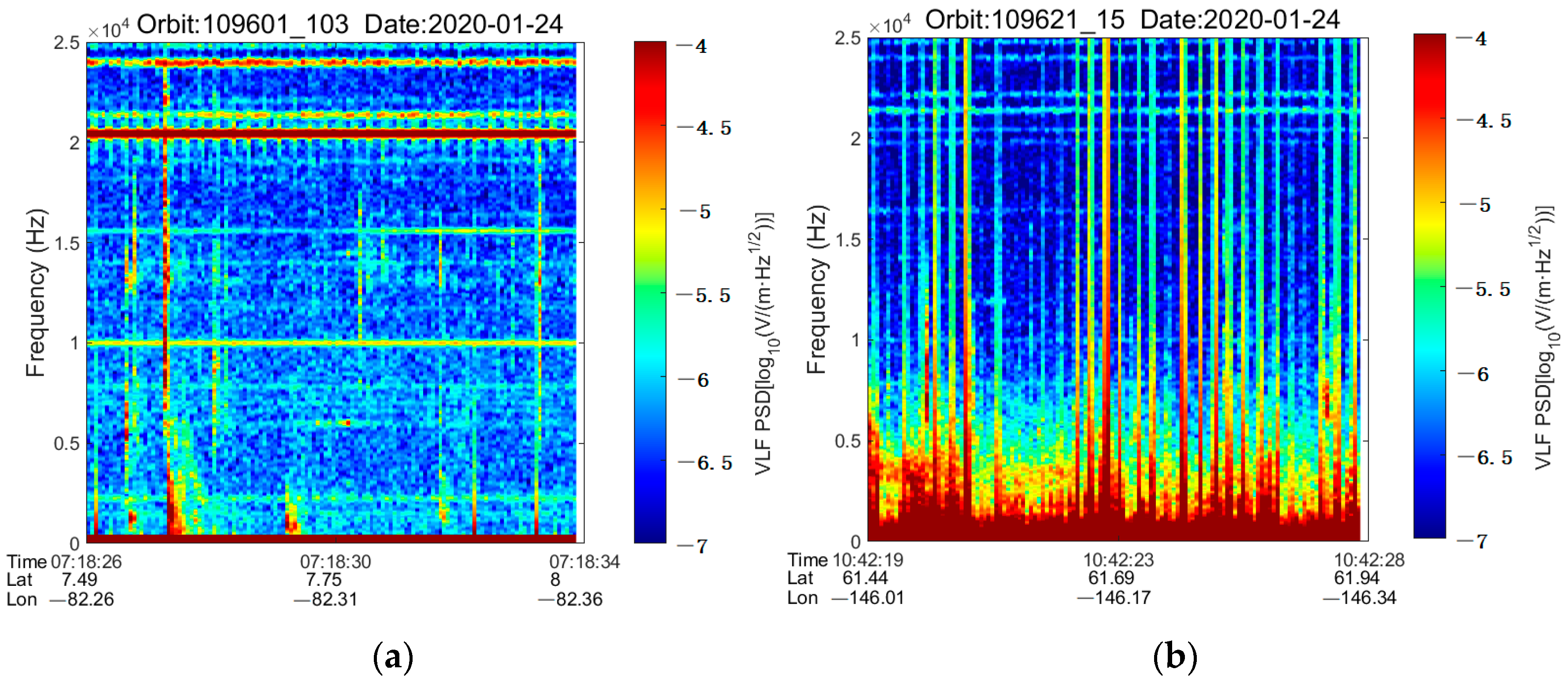
Figure 1. Two spectrograms with a duration of 8 s. (a) The 103rd spectrogram of orbit number 109601; (b) the 15th spectrogram of orbit number 109621.
Atmosphere 14 01296 g001
Figure 2. Flow chart of automatic recognition algorithm of VLPT. Among them, the yellow box represents the object handled in this article, the red box indicates the preprocessing process for the spectrogram, and the green box represents the workflow for unsupervised clustering.
Atmosphere 14 01296 g002
Figure 3. The result after grayscale conversion.
Atmosphere 14 01296 g003
Figure 4. Enhancement of vertical edge features.
Atmosphere 14 01296 g004
Figure 5. Binarization.
Atmosphere 14 01296 g005
Figure 6. When K = 2, an elbow occurs.
Atmosphere 14 01296 g006
Figure 7. Visualization of labeled straight lines after clustering.
Atmosphere 14 01296 g007
Figure 8. Recognition results marked on the grayscale.
Atmosphere 14 01296 g008
Figure 9. Step-by-step results of data preprocessing. (a) Original spectrogram; (b) grayscale; (c) vertical line feature enhancement; (d) binarization.
Atmosphere 14 01296 g009
Figure 10. Spectrograms of training samples. (a) A spectrogram which can be used as training samples after preprocessing; (b) visualization of the labels representing the vertical lines in the samples.
Atmosphere 14 01296 g010
Figure 11. Prediction on new samples. (a) Visualization of the labels representing the vertical lines in the new samples; (d) predicted results.
Atmosphere 14 01296 g011
Figure 12. Comparative analysis of different line recognition experiment results. (a) Original image; (b) Hough line recognition; (c) hierarchical clustering model; (d) DBScan model; (e) spectral clustering model; (f) K-means++ model after dimensionality reduction.
Atmosphere 14 01296 g012
Figure 13. The recognition results of different spectrograms, and the more column vectors representing line clusters there are, the greater the disturbance. (a) The results of line recognition; (b) the original spectrograms.
Atmosphere 14 01296 g013
Figure 14. A set of pulse sequence disturbances occurred in the latitude range (−8.65, −0.85) and longitude range (−79.27, −80.8) between 7:14:58 and 7:17:01 on 30 December 2019 from CSES with orbit number 105801.
Atmosphere 14 01296 g014aAtmosphere 14 01296 g014b
Figure 15. A set of pulse sequence disturbances occurred in the latitude range (−15.89, −3.83) and longitude range (−77.77, −80.17) between 7:12:52 and 7:16:02 on 4 January 2020 from CSES with orbit number 106561.
Atmosphere 14 01296 g015aAtmosphere 14 01296 g015b
Table 1. Statistical analysis of spectral clustering and improved K-means + + clustering Vertical lines recognition results.
Spectral ClusteringK-Means++
Accuracy (%)0.96 ± 0.010.98 ± 0.01
Missed Detection Rate (%)0.04 ± 0.010.02 ± 0.01
Error Rate (%)00
Time (s/per image)0.0420.013
Disclaimer/Publisher’s Note: The statements, opinions and data contained in all publications are solely those of the individual author(s) and contributor(s) and not of MDPI and/or the editor(s). MDPI and/or the editor(s) disclaim responsibility for any injury to people or property resulting from any ideas, methods, instructions or products referred to in the content.