Article

Estimation of the Concentration of XCO2 from Thermal Infrared Satellite Data Based on Ensemble Learning

1
College of Geomatics and Geoinformation, Guilin University of Technology, Guilin 541000, China
2
State Key Laboratory of Remote Sensing Science, Institute of Aerospace Information Innovation, Chinese Academy of Sciences, Beijing 100101, China
3
School of Electrical Engineering, Nantong University, Nantong 226019, China
*
Author to whom correspondence should be addressed.
Atmosphere 2024, 15(1), 118; https://doi.org/10.3390/atmos15010118
Submission received: 6 December 2023 / Revised: 8 January 2024 / Accepted: 10 January 2024 / Published: 19 January 2024
(This article belongs to the Section Atmospheric Techniques, Instruments, and Modeling)

Abstract

:
Global temperatures are continuing to rise as atmospheric carbon dioxide (CO2) concentrations increase, and climate warming has become a major challenge to global sustainable development. The Cross-Track Infrared Sounder (CrIS) instrument is a Fourier transform spectrometer with 0.625 cm−1 spectral resolution covering a 15 μm CO2-absorbing band, providing a way of monitoring CO2 with on a large scale twice a day. This paper proposes a method to predict the concentration of column-averaged CO2 (XCO2) from thermal infrared satellite data using ensemble learning to avoid the iterative computations of radiative transfer models, which are necessary for optimization estimation (OE). The training data set is constructed with CrIS satellite data, European Centre for Medium-Range Weather Forecasts (ECMWF) Reanalysis v5 (ERA5) meteorological parameters, and ground-based observations. The training set was processed using two methods: correlation significance analysis (abbreviated as CSA) and principal component analysis (PCA). Extreme Gradient Boosters (XGBoost), Extreme Random Trees (ERT), and Gradient Boost Regression Tree (GBRT) are used for training and learning to develop the new retrieval model. The results showed that the R2 of XCO2 prediction built from the PCA dataset was bigger than that from the CSA dataset. These three learning models were verified by validation sets, and the ERT model showed the best agreement between model predictions and the truth (R2 = 0.9006, RMSE = 0.7994 ppmv, MAE = 0.5804 ppmv). The ERT model was finally selected to estimate the concentrations of XCO2. The deviation of XCO2 predictions of 12 TCCON sites in 2019 was within ±1 ppm. The monthly averages of XCO2 concentrations in close agreement with TCCON ground observations were grouped into four regions: Asia (R2 = 0.9671, RMSE = 0.7072 ppmv), Europe (R2 = 0.9703, RMSE = 0.8733 ppmv), North America (R2 = 0.9800, RMSE = 0.6187 ppmv), and Oceania (R2 = 0.9558, RMSE = 0.4614 ppmv).

1. Introduction

Since the beginning of industrialisation, humanity’s pursuit of sustainable development has led to increasing greenhouse gas emissions. This significant rise in worldwide atmospheric carbon dioxide concentrations has escalated from 280 ppmv before the industrial revolution to 413.2 ppmv in 2020 [1]. The present extent of human-induced pollution and the unregulated release of greenhouse gases into the atmosphere have the potential to exacerbate signs of global climate change such as global warming, shifts in precipitation patterns, the thawing of glaciers, and the escalation of sea levels [2]. These issues have caused significant concern in the international community. In response to the challenge of climate change, the United Nations Paris Agreement was adopted at the 2015 Paris Climate Change Conference. The primary aim of the agreement is to restrict the rise in global average temperature, keeping it well below 2 °C, or even 1.5 °C [3]. Concerted efforts must be initiated to reduce carbon emissions and increase carbon sequestration through a range of socio-economic and technological interventions [2].
Concentrations of atmospheric trace gases are observed using spectrometers or air-sampling instruments. However, column-averaged concentrations are usually retrieved from spectrometers on the ground or onboard space aircraft. Ground-based measurements are effective in precisely determining trace gas concentrations. Nonetheless, the assessment of CO2 levels is limited by sparse spatial and temporal coverage [4]. In contrast, spaceborne measurements characterized by high spatiotemporal resolution are widely regarded as the most efficacious means of capturing spatial and temporal variations in CO2 distributions [5]. Satellite observations are suitable for “bottom-up” inversion to improve the accuracy of carbon sink estimations [6].
Thermal infrared (TIR) detectors [7] and near-infrared (NIR) detectors [8] are two primary methods of monitoring the concentration of CO2 in space. Thermal infrared hyperspectral sensors receive thermal radiation from the Earth’s surface, and are sensitive to the CO2 absorption in the mid to upper troposphere. In contrast, short-wave infrared detectors receive solar radiation reflected from surfaces, having sensitivities to CO2 absorption near the surface, but being affected by clouds and water vapour [9]. CrIS onboard NOAA-20, launched in 2017 and featuring accurate radiometric and spectral calibration, can provide observations in long time series. When considering a machine learning model to estimate CO2 concentrations, a sufficient number of samples can improve the model’s ability to generalize, reduce the risk of overfitting, and consequently improve the model’s predictive accuracy [10]. CrIS has much wider range than these SW IR sensors, and can provide more observations for modelling.
The physical retrieval model has commonly been used to estimate the concentrations of CO2 from satellite measurements. Zhang et al. [11] conducted a CO2 optimal estimation using CrIS full resolution spectral data, with an R2 of 0.72 and an RMSE of 0.45 ppmv when compared with measurements from the Civil Aircraft for the Regular Investigation of the Atmosphere Based on an Instrument Container (CARIBIC). The iterative inverse process is prone to nonconvergence due to the nonlinear radiation transfer equation and the difficulty of obtaining accurate atmospheric state parameters [12]. Zhao et al. [13] proposed a two-step machine learning model based on Greenhouse gases Observing SATellite (GOSAT) clear sky radiances, achieving a mean error (ME) of 0.09 ppmv and an RMSE of 3.13 ppmv, compared to GOSAT Level 2 product data. David et al. [14] proposed a neural network model (NN) for CO2 concentration estimation, with a precision of 0.8 ppmv, indicating that when trained on a representative dataset, the NN model offers slightly superior accuracy compared to the fully physical algorithm. This work demonstrated that both machine learning and neural network models can achieve high accuracy in predicting CO2 concentrations.
Ensemble learning is a meta-method that improves the performance of a model by combining multiple machine learning models, and mitigates the risk of overfitting often seen in machine learning algorithms when dealing with challenges like imbalanced, multidimensional, and noisy data [15]. This approach can improve the overall forecast accuracy and stability. In this paper, we employed three models to predict the concentration of XCO2 from thermal infrared satellite data using ensemble learning. The dataset used for training was constructed using CrIS satellite data, ERA5 meteorological parameters, the normalised difference vegetation index (NDVI), surface parameters, DEM, and ground-based observations; the training set was processed using two methods: correlation significance analysis and principal component analysis (PCA). Comparing between model predictions and the truth in three ensemble learning algorithm models, we identified the most suitable model for estimating CO2 concentrations using thermal infrared data. This research provides a precise and efficient model algorithm for CO2 concentration estimation.

2. Data Sources and Processing

2.1. Data Sources

We used column-averaged concentrations of CO2 from TCCON sites as reference benchmarks to build the dataset and validate the accuracy of the model [16]. Parameters were derived from CrIS, ERA5, and products from other satellites for describing representative features in spectral, spatial-temporal, meteorological and surface domains.

2.1.1. TCCON Data

The Total Carbon Column Observing Network (TCCON) is a global observational network that gathers high-precision atmospheric greenhouse gas (primarily CO2 and CH4) concentrations from ground-based Fourier transform spectrometers. TCCON was established in 2004, and has expanded from its initial 3 sites to the current 26 official sites [17]. Figure 1 illustrates the distribution of TCCON sites, primarily located in North America, Europe, and the East Asia.
The concentrations of XCO2 were processed with the Gas Fit (GFIT) algorithm, a non-linear least-squares fitting method [18], which involves generating a synthetic spectrum by fine-tuning a priori profiles to achieve the closest match with the observed spectrum. The total column amounts of CO2 were integrated from the adjusted CO2 profile, and the concentrations of XCO2 were divided by the total column amount of dry air [19]. This study used the latest version of the TCCON data (GGG 2020) [20], from all 26 sites in 2019. The detailed information of TCCON sites is listed in Table 1.

2.1.2. CrIS

The Joint Polar Satellite System-1 (JPSS-1) satellite was successfully launched into space from Vandenberg Air Force Base on 18 November 2017. Mounted on the satellite, the CrIS (Cross-track Infrared Sounder) is a Fourier-transform infrared spectrometer equipped with a total of 2211 infrared detection channels. ATMS (Advanced Technology Microwave Sounder) is a microwave sensor with 22 channels, operating within a frequency range from 23 GHz to 183 GHz. The CLIMCAPS (Community Long-Term Infrared Microwave Coupled Product System) algorithm was employed for the analysis of the infrared and microwave well-calibrated radiance of this CrIS/ATMS. Due to the significant impact of clouds on observations from the infrared detector, cloud-clearing processing was applied, yielding cloud-cleared radiance L2 products, which provides radiation that is free of cloud and fog interference. The data are generated at 6 min intervals, covering 30 positions horizontally and having 45 data points along the orbit. With a spatial resolution of 50 km, this dataset has one of the highest spatial and temporal resolutions of the data sets currently available for meteorological analysis [21,22,23].

2.1.3. ERA5

The European Centre for Medium-Range Weather Forecasts (ECMWF) Reanalysis v5 (ERA5) is a fifth-generation global climate reanalysis dataset. It provides high-spatial-resolution and high-temporal-resolution meteorological fields worldwide, including various meteorological and cloud parameters such as temperature, precipitation, wind speed, and atmospheric pressure. ERA5 features a spatial resolution of 0.25° and a temporal resolution of 1 h, establishing its status as the most high-resolution global meteorological reanalysis dataset available to date [24].
To further investigate the influence of cloud and meteorological features on CO2 concentration, this study acquired meteorological parameters including temperature, wind components (U and V), and vertical velocity within the pressure range of 100 to 1000 hPa. Additionally, data related to cloud features were collected, including boundary layer height (blh), cloud base height (cbh), total cloud cover (tcc), and total precipitation (tp). Furthermore, gas-related data, such as total ozone column concentration (tco3) in the atmosphere, were also obtained.

2.1.4. Other Parameters

The normalized difference vegetation index (NDVI) is an indicator used to assess the extent of vegetation coverage and its growth conditions. The concentration of CO2 is highly affected by the condition of surface vegetation [25]. In this work, NDVI values were extracted from MODIS (MOD13Q1 [26]) with a spatial resolution of 250 m and a temporal resolution of 16 days.
Surface parameters such as surface emissivity and skin temperature are crucial for upward atmospheric radiation [27,28]. In this work, the surface reflectance was extracted from MODIS (MOD09GA [29]), in the infrared band (620–670 nm) with a spatial resolution of 500 m.
There is also a certain relationship between site elevation and XCO2 concentration. Additionally, the elevation was extracted from Global Land One km Base Elevation (GLOBE) (GLOBE Topography [30]) with a spatial resolution of 1 km.

2.2. Data Processing

TCCON carries out continuous measurements of data at 90 s intervals on a daily basis. For each TCCON site, we calculated the mean and standard deviation of XCO2 concentrations. Then, we removed the data that exceed three times the standard deviation. Finally, we recomputed the mean of the remaining values to obtain the corrected daily XCO2 concentration for each site [13]. The processing of parameters as trained by CrIS included the following operations. (1) The reciprocal of the cosine of the solar zenith angle and the zenith angle were found, respectively, and the sine of the difference between the solar azimuth angle and the satellite azimuth angle was found. (2) The spectral channels were selected in the range of 648.75 cm−1 to 1096.875 cm−1, giving a total of 717 channels. Due to variations in the temporal and spatial resolutions of the parameters involved in the modelling process, it was necessary to perform spatiotemporal matching. This involved standardizing the data to a daily temporal resolution and a spatial resolution of 1° [17]. We performed daily averaging on the hourly data provided by ERA5 meteorological reanalysis. The MODIS NDVI and surface reflectance data have different temporal resolutions (16 days and daily, respectively). These parameters used daily column-averaged CO2 concentrations from TCCON sites as reference benchmarks to build the dataset. The specific information of the features used for model training is listed in Table 2.

3. Methodology

Machine learning is a branch of artificial intelligence whose primary aim is to enable computers to automatically learn from data and use the acquired knowledge for prediction or decision making [31]. Models in machine learning are mathematical algorithms that learn from data to make predictions, classifications, or decisions on unseen data by identifying patterns and relationships in the information; many machine learning models have been developed and are widely used, including neural networks (NNs), random forest (RF), support vector machines (SVMs), convolutional neural networks (CNNs), etc. [32]. Ensemble learning has shown good consistency in gas concentration inversion studies [33]. This study analyses and compares three ensemble learning algorithms: Gradient Boosting Decision Trees (XGBoost), Gradient Boosting Regression Trees (GBRT), and Extremely Randomized Trees (ERT), with the aim of selecting the optimal estimation model.

3.1. Ensemble Learning Methods

Ensemble learning is a machine learning approach whose core idea is to enhance the overall performance and robustness of a model by combining the predictions of multiple individual models [34]. Ensemble learning methods are primarily divided into two main categories: bagging and boosting. Bagging involves the creation of many subsamples through random sampling with replacement. Each of these subsamples is then utilized to train an individual base model. The final prediction results from these models are combined through averaging or voting [35]. By contrast, boosting modifies the weights of the samples in each iteration, based on the prediction errors from the previous stage; the final ensemble model is ultimately obtained by aggregating the predictions of all the base models through weighted combination [36]. By combining predictions from several models, ensemble learning can efficiently employ different models’ strengths, address individual models’ weaknesses, and improve prediction accuracy and generalization capabilities. This approach has been demonstrated in practical applications to significantly enhance model performance, making it adaptable to a broader range of data and problems [37].
Extreme Gradient Boosting (XGBoost) stands out as an optimized distributed gradient boosting algorithm, notable for its expedited computational performance compared to contemporary popular machine learning models. This model incorporates a regularization term within the loss function to manage the model’s complexity. The adjusted loss function is elucidated through the utilization of the two-dimensional Taylor formula. This strategic refinement effectively addresses the issues of overfitting inherent in conventional gradient boosting models, concurrently augmenting the model’s accuracy and its generalization capabilities [38]. Gradient Boosted Regression Trees (GBRT) constitute a supervised machine learning technique that was first conceptualized by Friedman in 2001. It embodies the concept of a robust learner, weighted by an ensemble of multiple weaker learners. Each of the weaker learners is represented as an individual regression decision tree, and every subtree is oriented toward learning in the direction of the negative gradient associated with the residuals from the preceding tree. Through continuous iterations aimed at minimizing the loss function, the GBRT prediction model is systematically forged. The algorithm predominantly comprises the stages of expanding regression decision trees, judiciously pruning these trees and harmoniously amalgamating them into a coherent ensemble [39]. Compared with traditional random forest, Extremely Randomized Trees (ERT) employ the entire dataset to train individual decision trees. This ensures the effective utilization of training samples and contributes to a reduction in the final prediction bias. To maintain distinct structural variations among each decision tree, ERT introduces increased randomness to node splitting. Specifically, it involves the random selection of division thresholds for each feature from the sub-dataset, and the optimal partition attribute is chosen based on the best division according to the specified threshold feature [40].

3.2. Model Evaluation Methodology

The model’s performance was evaluated using the squared coefficient of determination (R2), which determines the extent to which the model explains the variance in the observations [41]. Furthermore, the root mean square error (RMSE) was used to illustrate the standard deviation of residuals (prediction error) [42], whereas the mean absolute error (MAE) calculated the average absolute difference between model predictions and observed values [43]. The TCCON observation was set as yi y ¯ i is the mean of the TCCON observation,  y ^ i is the model prediction, and n is the number of samples.
R 2  is computed as follows:
R 2 = 1 i = 1 n ( y i y ^ i ) 2 i = 1 n ( y i y ¯ i ) 2
The  R M S E  is the square root of the mean of the squared deviations between predicted values and observed values. The formula is as follows:
R M S E = = i = 1 n ( y i y ^ i ) 2 n
The  M A E  is the mean of the absolute disparities between predicted values and observation values. The formula is as follows:
M A E = 1 n i = 1 n | y i y ^ i |

3.3. Technical Flowchart

The estimation process of the concentration of XCO2 from thermal infrared satellite data based on ensemble learning in the thermal infrared is shown in Figure 2. Firstly, the data were standardized to a daily temporal resolution and a unique spatial resolution of 1°. Due to the large number of features, two methods were employed to construct datasets to select the optimal feature parameters: correlation significance analysis and principal component analysis. The datasets were randomly divided into training sets (80%), testing sets (10%), and validation sets (10%). Three different ensemble learning models (ERT, XGBoost, GBRT) were employed and compared over two datasets. The final objective is to choose the model with the lowest RMSE in the estimation of XCO2 concentration.

4. Feature and Model Experiments

This study employed correlation and significance analysis and principal component analysis (PCA) to select the characteristic variables. Improving training speed by reducing features and reducing interference noise to reduce the risk of overfitting improves model effectiveness, we chose a training set that is more suitable for building an ensemble learning model. The experiments were carried out using XGBoost, GBRT, and ERT with two datasets.

4.1. Correlation and Significance Analysis

Correlation and significance analysis can be employed to filter out unimportant features, reduce the number of features, enhance model accuracy, and reduce runtime. The Pearson correlation coefficient is typically denoted as “r”, and is used as a statistical measurement to assess the strength of the linear relationship between two continuous variables [44]. Significance is commonly represented using p-values and is also used to filter out unimportant features [45].
In Figure 3, the heat map of correlation coefficients shows a positive correlation in red and a negative correlation in blue, and the number of stars shows the level of significance. Sensitivity was assessed in each case by examining the correlation coefficient® and its level of statistical significance (p-value). XCO2 showed a positive correlation with lat, DEM, blh, cl, and tco3, with a significance of 0.01. Among these factors, tco3 has the highest positive correlation, which is 0.27. XCO2 showed a negative correlation with lon, month, dd, NDVI, skt, and t2m, and NDVI showed the highest negative correlation of −0.21. Other features exhibited low or no correlation with XCO2, so they were all removed. Ultimately, lat, lon, month, dd, NDVI, skt, t2m, DEM, blh, cl, and tco3 were retained. The selection of spectral bands involved choosing two channels around 15 µm that are sensitive to CO2 but not sensitive to other variables, based on the Jacobian function, as mentioned in [11]. Figure 4 illustrates the selected bands, denoted by red lines. The final selected two spectral bands corresponded to radiance at wavelengths of 668.75 cm−1 and 701.875 cm−1.

4.2. Principal Component Analysis

Principal component analysis (PCA) is a widely used method for data dimensionality reduction and extracting essential information [46]. This process involves finding a new set of orthogonal feature vectors, also known as principal components, that capture the variability in the original data in a particular way, allowing for an efficient representation of the data in lower dimensions while maximising the retention of information in the data. By selecting an appropriate number of principal components, it is possible to achieve dimensionality reduction in the data, reducing redundancy and enabling a deeper understanding and analysis of the data [47].
In this work, principal component analysis was conducted on 717 channels within the spectral range of 648.75 cm−1 to 1096.875 cm−1 which had information on CO2 absorption, and the first three principal components scores were computed to represent the information from 717 channels. Similarly, principal component analysis was conducted on meteorological data on ten pressures (100–1000 hPa), and temperature (T), vertical wind speed (U), horizontal wind speed (V), vertical wind speed (W) on these ten pressures, and the first three principal components were selected to represent meteorological data. Additionally, one principal component was chosen to represent satellite observed geometry information. Additionally, surface parameters such as NDVI, SR, and DEM have become crucial for the upward atmospheric radiation. The initial dataset was constructed by employing spatial–temporal and spectral characteristics as reference benchmarks. This study investigates the influence of additional parameters on model correctness through the utilization of the ERT model. Figure 5 illustrates the values of R2, RESE, and MAE for the ERT model that was trained using various features. The results demonstrated that the features such as NDVI, SR, and PCA scores of the observed geometry information of satellites (abbreviated as SOA) resulted in a noteworthy enhancement of the R2 value of the model. Furthermore, a decrease in RMSE and MAE values suggested a favourable impact of these features on the overall performance of the model. The first three principal components score of meteorological data and DEM exhibited a minimal or negligible impact on the accuracy of the model. Consequently, these features were excluded from the dataset.

4.3. Model Training Comparison

Three distinct ensemble learning models, namely ERT, XGBoost, and GBRT, were utilized for training. The determination of the optimal selection of primary parameters for the three ensemble learning models was achieved by optimizing model parameters. The model parameter settings can be found in Table 3. The adjustment of parameter configurations will improve the performance of the model during both the training and prediction stages, hence guaranteeing more precise and dependable forecasting outcomes [48].
Figure 6 showed a scatter plot of the XCO2 concentration of the three different ensemble learning models (ERT, XGBoost, GBRT), with datasets derived from the testing dataset. Comparing these three models, the R2 of XCO2 prediction built from the PCA was found to be significantly higher than that from the correlation and significance analysis. The ERT model demonstrated the best agreement (as shown in Table 4), with an R2 of 0.9231, an RMSE of 0.7552 ppmv, and a MAE of 0.5568 ppmv. The result showed that the R2 of the ERT model was higher, and the RMSE and MAE were lower than those of the other models.

5. Validation

Figure 7 shows a scatter plot of predicted XCO2 concentration in the validation set. These three learning models were validated using validation sets. The results show that the R2 values were 0.9006, 0.8720, and 0.8769 for ERT, GBRT, and XGBoost, respectively. The RMSE values were 0.7994, 0.9068, and 0.8897, and the MAE values were 0.5804, 0.6705, and 0.6624(as shown in Table 5). The ERT had the highest R2 and the lowest RMSE and MAE. Combining these with consideration of three model evaluation indicators, the ERT model showed the best agreement in model validation, with high prediction accuracy and minimal prediction errors. Thus, the ERT model was finally selected to estimate the concentrations of XCO2.
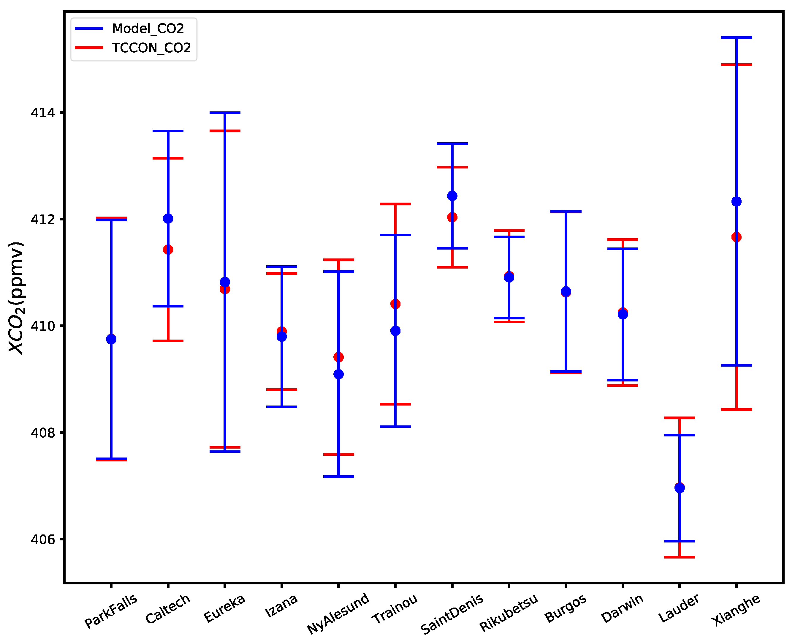
The mean and standard deviation of the XCO2 concentrations obtained from 12 TCCON stations in the validation set were compared with the XCO2 concentrations predicted by the ERT model in Figure 8. The Xianghe station in China exhibited the highest concentration of XCO2, as indicated by a model projected value of 412.33 ppmv and an observed value of 412.17 ppmv. The Lauder station in New Zealand exhibited the lowest concentration of XCO2, as evidenced by the observed value of 406.86 ppmv compared to the model projected value of 406.96 ppmv. The mean and standard deviations of XCO2 concentrations at various stations were within ±1 ppmv. The results indicate that the XCO2 concentrations at various longitudes and latitudes were accurately predicted by the ERT model.
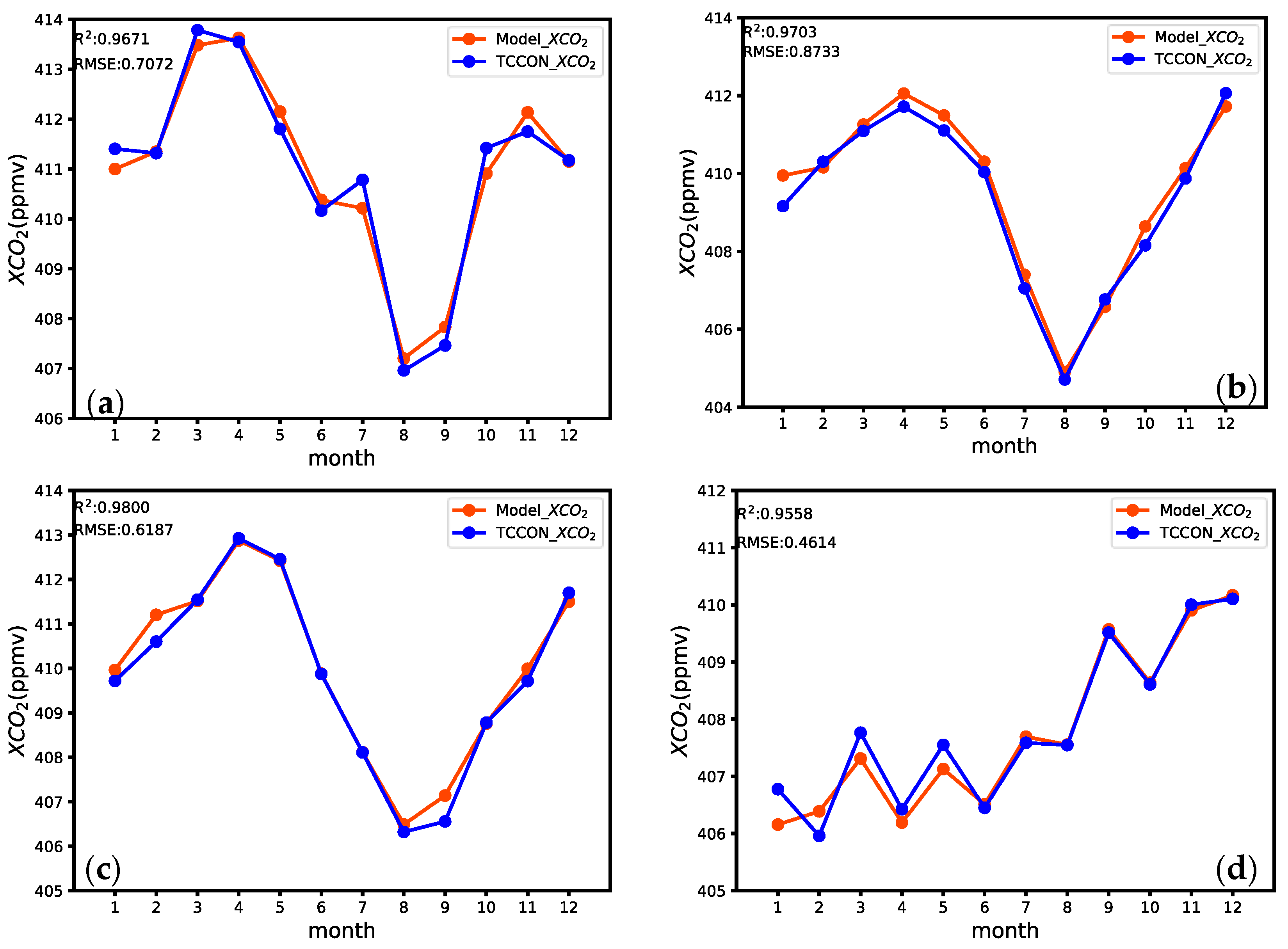
Based on the global distribution of TCCON sites, the results of ground-based observations and model predictions were categorized into four groups: such as Asia, Europe, South America, and Oceania. The model predicted results were compared with the monthly means and standard deviations of the TCCON measurements (as shown in Figure 9). The R2 and RMSE values for the monthly mean values of TCCON observations and model predictions are as follows in the four regions: Asia (R2 = 0.9671, RMSE = 0.7072 ppmv), Europe (R2 = 0.9703, RMSE = 0.8733 ppmv), North America (R2 = 0.9800, RMSE = 0.6187 ppmv), and Oceania (R2 = 0.9558, RMSE = 0.4614 ppmv). The monthly averages of XCO2 concentrations of model prediction and TCCON observations are generally consistent in the four regions. The concentration of XCO2 at the sites located in Asia, Europe, and North America demonstrate a declining pattern throughout June to August, followed by a steady increase in the subsequent months from August to December.
The model prediction exhibits significant agreement with the TCCON observations in most months, notably in the trends of XCO2 concentration seasonal fluctuations during the summer and autumn. The results suggest that the model exhibits a strong ability to estimate XCO2 concentrations on a monthly basis. However, the accuracy of model predictions in the Oceania region is limited due to a lack of samples.

6. Conclusions

In this work, three ensemble learning models were used for the prediction of column-averaged CO2 concentrations from thermal infrared satellite data. These estimations were based on data obtained from the CrIS satellite, ERA5 meteorological parameters, and ground-based observations. The study involved a comparison of datasets generated using two methodologies in order to identify the most suitable model. Research indicates the following conclusions:
(1) The primary determinants affecting the evaluation of the concentration of XCO2, as studied through correlation and significance analysis, encompass latitude, NDVI, and TCO3. The correlations between XCO2 and these variables are 0.18, −0.17, and 0.26, showing a strong correlation between the concentration of CO2 and the seasonal variation in biomass. The PCA showed that the features such as NDVI, SR, and PCA scores of the observed geometry information of satellites could raise up the R2 of the model. The NDVI showed a substantial influence on both datasets and warranted careful consideration as a pivotal feature in forthcoming CO2 retrieval procedures.
(2) The dataset constructed using PCA leads to improved accuracy in the estimation of XCO2 concentrations. The ERT model demonstrated the highest estimation accuracy based on several evaluation indicators, including an R2 value of 0.9231, an RMSE value of 0.7552 ppmv, and an MAE value of 0.5568 ppmv.
(3) The model predictions agree well with the measurements from the TCCON sites in industrial regions, including Xianghe, Saint Denis and Caltech, showing higher XCO2 concentrations than other sites. The examination of monthly trends indicates the existence of seasonal variations in XCO2 levels across multiple sites in Asia, Europe, and North America. It is worth noting that the lowest concentration of XCO2 appears in August. TCCON station observations have high precision, but the scarcity of globally effective observation sites results in very limited observational data. Looking ahead, as the number of observation sites continues to grow, our model presents a valuable tool for estimating regional CO2 concentrations. Furthermore, it enables the analysis of spatiotemporal variations in CO2 concentrations, particularly focusing on key urban areas. This research contributes to the broader understanding of carbon dioxide dynamics, aiding in the development of targeted strategies for environmental management and policy formulation.

Author Contributions

Conceptualization, X.G.; methodology, X.G. and X.Z.; formal analysis, X.G.; investigation, X.G., Y.Z. and S.S.; data curation, X.G. and Y.Z.; writing—original draft, X.G.; writing—review and editing, X.G., Y.Z. and Z.L., visualization, X.G.; supervision, Y.Z. and M.F. All authors have read and agreed to the published version of the manuscript.

Funding

This research was financially supported by the National Key Research and Development Plan (Grant No. 2021YFB3901000).

Institutional Review Board Statement

Not applicable.

Informed Consent Statement

Not applicable.

Data Availability Statement

XCO2 remote sensing data: Cross-Track Infrared Sounder (CrIS) satellite data: https://www.avl.class.noaa.gov/saa/products/ (accessed on 2 December 2022). European Centre for Medium-Range Weather Forecasts (ECMWF) Reanalysis v5 (ERA5) meteor-ological parameters: https://www.ecmwf.int/en/forecasts/datasets/reanalysis-datasets/era5/ (accessed on 1 December 2022). XCO2 measurements data: TCCON: https://tccondata.org/2020 (accessed on 2 December 2022).

Conflicts of Interest

The authors declare no conflict of interest.

References

  1. Liu, L.Y.; Chen, L.F. Satellite remote sensing for global stocktaking: Methods, progress and perspectives. Natl. Remote Sens. Bull. 2022, 26, 243–267. [Google Scholar] [CrossRef]
  2. Yoro, K.O.; Daramola, M.O. CO2 emission sources, greenhouse gases, and the global warming effect. In Advances in Carbon Capture; Woodhead Publishing: Cambridge, UK, 2020; pp. 3–28. [Google Scholar]
  3. Rogelj, J.; Huppmann, D.; Krey, V.; Riahi, K.; Clarke, L.; Gidden, M.; Nicholls, Z.; Meinshausen, M. A new scenario logic for the Paris Agreement long-term temperature goal. Nature 2019, 573, 357–363. [Google Scholar] [CrossRef]
  4. Houweling, S.; Hartmann, W.; Aben, I.; Schrijver, H.; Skidmore, J.; Roelofs, G.J.; Breon, F.M. Evidence of systematic errors in SCIAMACHY-observed CO2; due to aerosols. Atmos. Chem. Phys. 2005, 5, 3003–3013. [Google Scholar] [CrossRef]
  5. Baker, D.F.; Bösch, H.; Doney, S.C.; O’Brien, D.; Schimel, D.S. Carbon source/sink information provided by column CO2 measurements from the Orbiting Carbon Observatory. Atmos. Chem. Phys. 2010, 10, 4145–4165. [Google Scholar] [CrossRef]
  6. Wang, Y.; Wang, X.; Wang, K.; Chevallier, F.; Zhu, D.; Lian, J.; He, Y.; Tian, H.; Li, J.; Zhu, J.; et al. The size of the land carbon sink in China. Nature 2022, 603, E7–E9. [Google Scholar] [CrossRef] [PubMed]
  7. Rogalski, A. Recent progress in infrared detector technologies. Infrared Phys. Technol. 2011, 54, 136–154. [Google Scholar] [CrossRef]
  8. Suto, H.; Kataoka, F.; Kikuchi, N.; Knuteson, R.O.; Butz, A.; Haun, M.; Buijs, H.; Shiomi, K.; Imai, H.; Kuze, A. Thermal and near-infrared sensor for carbon observation Fourier transform spectrometer-2 (TANSO-FTS-2) on the Greenhouse gases Observing SATellite-2 (GOSAT-2) during its first year in orbit. Atmos. Meas. Tech. 2021, 14, 2013–2039. [Google Scholar] [CrossRef]
  9. Chen, L.F.; Zhang, Y. Overview of atmospheric CO2 remote sensing from space. Natl. Remote Sens. Bull. 2015, 19, 1–11. [Google Scholar]
  10. Ying, X. An Overview of Overfitting and its Solutions. J. Phys. Conf. Ser. 2019, 1168, 022022. [Google Scholar] [CrossRef]
  11. Zhang, X.; Zhang, Y.; Bai, L.; Tao, J.; Chen, L.; Zou, M.; Han, Z.; Wang, Z. Retrieval of Carbon Dioxide Using Cross-Track Infrared Sounder (CrIS) on S-NPP. Remote Sens. 2021, 13, 1163. [Google Scholar] [CrossRef]
  12. Li, J.B.; Zhang, Y.; Gai, R.L. CO2 satellite inversion method based on machine learning for short wave infrared channel. China Environ. Sci. 2023, 43, 1499–1509. [Google Scholar]
  13. Zhao, Z.; Xie, F.; Ren, T.; Zhao, C. Atmospheric CO2 retrieval from satellite spectral measurements by a two-step machine learning approach. J. Quant. Spectrosc. Radiat. Transf. 2022, 108006. [Google Scholar] [CrossRef]
  14. David, L.; Bréon, F.-M.; Chevallier, F. XCO2 estimates from the OCO-2 measurements using a neural network approach. Atmos. Meas. Tech. 2020, 14, 117–132. [Google Scholar] [CrossRef]
  15. Dong, X.; Yu, Z.; Cao, W.; Shi, Y.; Ma, Q. A survey on ensemble learning. Front. Comput. Sci. 2019, 14, 241–258. [Google Scholar] [CrossRef]
  16. He, Q.; Ye, T.; Chen, X.; Dong, H.; Wang, W.; Liang, Y.; Li, Y. Full-coverage mapping high-resolution atmospheric CO2 concentrations in China from 2015 to 2020: Spatiotemporal variations and coupled trends with particulate pollution. J. Clean. Prod. 2023, 428, 139290. [Google Scholar] [CrossRef]
  17. Messerschmidt, J.; Geibel, M.C.; Blumenstock, T.; Chen, H.; Deutscher, N.M.; Engel, A.; Feist, D.G.; Gerbig, C.; Gisi, M.; Hase, F.; et al. Calibration of TCCON column-averaged CO2: The first aircraft campaign over European TCCON sites. Atmos. Chem. Phys. 2011, 11, 10765–10777. [Google Scholar] [CrossRef]
  18. Wunch, D.; Toon, G.C.; Blavier, J.F.L.; Washenfelder, R.A.; Notholt, J.; Connor, B.J.; Griffith, D.W.T.; Sherlock, V.; Wennberg, P.O. The total carbon column observing network. Philos. Trans. R. Soc. A 2011, 369, 2087–2112. [Google Scholar] [CrossRef]
  19. Dupuy, E.; Morino, I.; Deutscher, N.M.; Yoshida, Y.; Uchino, O.; Connor, B.J.; De Mazière, M.; Griffith, D.W.T.; Hase, F.; Heikkinen, P.; et al. Comparison of XH2O Retrieved from GOSAT Short-Wavelength Infrared Spectra with Observations from the TCCON Network. Remote Sens. 2016, 8, 414. [Google Scholar] [CrossRef]
  20. Total Carbon Column Observing Network (TCCON) Team. 2020 TCCON Data Release; CaltechDATA: Pasadena, CA, USA, 2022. [Google Scholar] [CrossRef]
  21. Fu, D.; Bowman, K.W.; Worden, H.M.; Natraj, V.; Worden, J.R.; Yu, S.; Veefkind, P.; Aben, I.; Landgraf, J.; Strow, L.; et al. High-resolution tropospheric carbon monoxide profiles retrieved from CrIS and TROPOMI. Atmos. Meas. Tech. 2016, 9, 2567–2579. [Google Scholar] [CrossRef]
  22. Gambacorta, A.; Barnet, C.D. Methodology and Information Content of the NOAA NESDIS Operational Channel Selection for the Cross-Track Infrared Sounder (CrIS). IEEE Trans. Geosci. Remote Sens. 2013, 51, 3207–3216. [Google Scholar] [CrossRef]
  23. Smith, N.; Barnet, C.D. Uncertainty characterization and propagation in the community long-term infrared microwave combined atmospheric product system (CLIMCAPS). Remote Sens. 2019, 11, 1227. [Google Scholar] [CrossRef]
  24. Wang, H.; Wang, Y.; Cai, K.; Zhu, S.; Zhang, X.; Chen, L. Evaluating the performance of ozone products derived from CrIS/NOAA20, AIRS/aqua and ERA5 reanalysis in the polar regions in 2020 using ground-based observations. Remote Sens. 2021, 13, 4375. [Google Scholar] [CrossRef]
  25. He, Z.; Lei, L.; Zeng, Z.C.; Sheng, M.; Welp, L.R. Evidence of carbon uptake associated with vegetation greening trends in eastern China. Remote Sens. 2020, 12, 718. [Google Scholar] [CrossRef]
  26. MOD13GA. Available online: https://ladsweb.modaps.eosdis.nasa.gov/missions-and-measurements/products/MOD13GA (accessed on 5 March 2022).
  27. Yang, J.; Yao, Y.; Wei, Y.; Zhang, Y.; Jia, K.; Zhang, X.; Shang, K.; Bei, X.; Guo, X. A Robust Method for Generating High-Spatiotemporal-Resolution Surface Reflectance by Fusing MODIS and Landsat Data. Remote Sens. 2020, 12, 2312. [Google Scholar] [CrossRef]
  28. Zhao, L.; Chen, S.; Xue, Y.; Cui, T. Study of Atmospheric Carbon Dioxide Retrieval Method Based on Normalized Sensitivity. Remote Sens. 2022, 14, 1106. [Google Scholar] [CrossRef]
  29. MOD13Q1. Available online: https://ladsweb.modaps.eosdis.nasa.gov/missions-and-measurements/products/MOD13Q1 (accessed on 20 March 2022).
  30. National Geophysical Data Center. Global Land One-km Base Elevation Project (GLOBE Topography); National Geophysical Data Center: Boulder, Colorado, 1999. [Google Scholar]
  31. Kumar, Y.; Kaur, K.; Singh, G. Machine learning aspects and its applications towards different research areas. In Proceedings of the 2020 International Conference on Computation, Automation and Knowledge Management (ICCAKM), Dubai, United Arab Emirates, 9–10 January 2020; pp. 150–156. [Google Scholar]
  32. Zhang, M.; Liu, G. Mapping contiguous XCO2 by machine learning and analyzing the spatio-temporal variation in China from 2003 to 2019. Sci. Total Environ. 2023, 858, 159588. [Google Scholar] [CrossRef] [PubMed]
  33. Song, S.P.; Fan, M. Estimating ground-level ozone concentration in China using ensemble learning methods. Natl. Remote Sens. Bull. 2023, 27, 1792–1806. [Google Scholar]
  34. Kunapuli, G. Ensemble Methods for Machine Learning; Simon and Schuster: New York City, NY, USA, 2023. [Google Scholar]
  35. Tang, W.Y.; Zhou, Z.H. Bagging-based selective clusterer ensemble. J. Softw. 2005, 16, 496–502. [Google Scholar] [CrossRef]
  36. Yu, L.; Wu, D.J. Assemble Learning: A Survey of Boosting Algorithms. Pattern Recognit. Artif. Intell. 2004, 17, 52–59. [Google Scholar]
  37. Polikar, R. Ensemble learning. In Ensemble Machine Learning: Methods and Applications; Springer: New York, NY, USA, 2012; pp. 1–34. [Google Scholar]
  38. Chen, T.; Guestrin, C. XGBoost: A scalable tree boosting system. In Proceedings of the ACM SIGKDD International Conference on Knowledge Discovery and Data Mining, San Francisco, CA, USA, 13–17 August 2016; Association for Computing Machinery: New York, NY, USA, 2016; pp. 785–794. [Google Scholar]
  39. Xu, S.; Ni, C.; Hu, X. Predicting Terrestrial Heat Flow in North China Using Multiple Geological and Geophysical Datasets Based on Machine Learning Method. Energies 2023, 16, 1620. [Google Scholar] [CrossRef]
  40. He, S.; Yuan, Y.; Wang, Z.; Luo, L.; Zhang, Z.; Dong, H.; Zhang, C. Machine Learning Model-Based Estimation of XCO2 with High Spatiotemporal Resolution in China. Atmosphere 2023, 14, 436. [Google Scholar] [CrossRef]
  41. Nagelkerke, N.J.D. A note on a general definition of the coefficient of determination. Biometrika 1991, 78, 691–692. [Google Scholar] [CrossRef]
  42. Chai, T.; Draxler, R.R. Root mean square error (RMSE) or mean absolute error (MAE)—Arguments against avoiding RMSE in the literature. Geosci. Model Dev. 2014, 7, 1247–1250. [Google Scholar] [CrossRef]
  43. Hodson, T.O. Root-mean-square error (RMSE) or mean absolute error (MAE): When to use them or not. Geosci. Model Dev. 2022, 15, 5481–5487. [Google Scholar] [CrossRef]
  44. Armstrong, R.A. Should Pearson’s correlation coefficient be avoided. Ophthalmic Physiol. Opt. 2019, 39, 316–327. [Google Scholar] [CrossRef]
  45. Goïta, K.; Magagi, R.; Beauregard, V.; Wang, H. Retrieval of Surface Soil Moisture over Wheat Fields during Growing Season Using C-Band Polarimetric SAR Data. Remote Sens. 2023, 15, 4925. [Google Scholar] [CrossRef]
  46. Frappart, F.; Ramillien, G.; Seoane, L. Monitoring Water Mass Redistributions on Land and Polar Ice Sheets Using the GRACE Gravimetry from Space Mission. In Land Surface Remote Sensing in Continental Hydrology; Elsevier: Amsterdam, The Netherlands, 2016; pp. 255–279. [Google Scholar]
  47. Song, W.; Han, X.; Qi, J. Prediction of Gas Emission in the Working Face Based on LASSO-WOA-XGBoost. Atmosphere 2023, 14, 1628. [Google Scholar] [CrossRef]
  48. Stephen, B.; Hastie, T.; Tibshirani, R. Cross-validation: What does it estimate and how well does it do it. J. Am. Stat. Assoc. 2023, 1–12. [Google Scholar] [CrossRef]
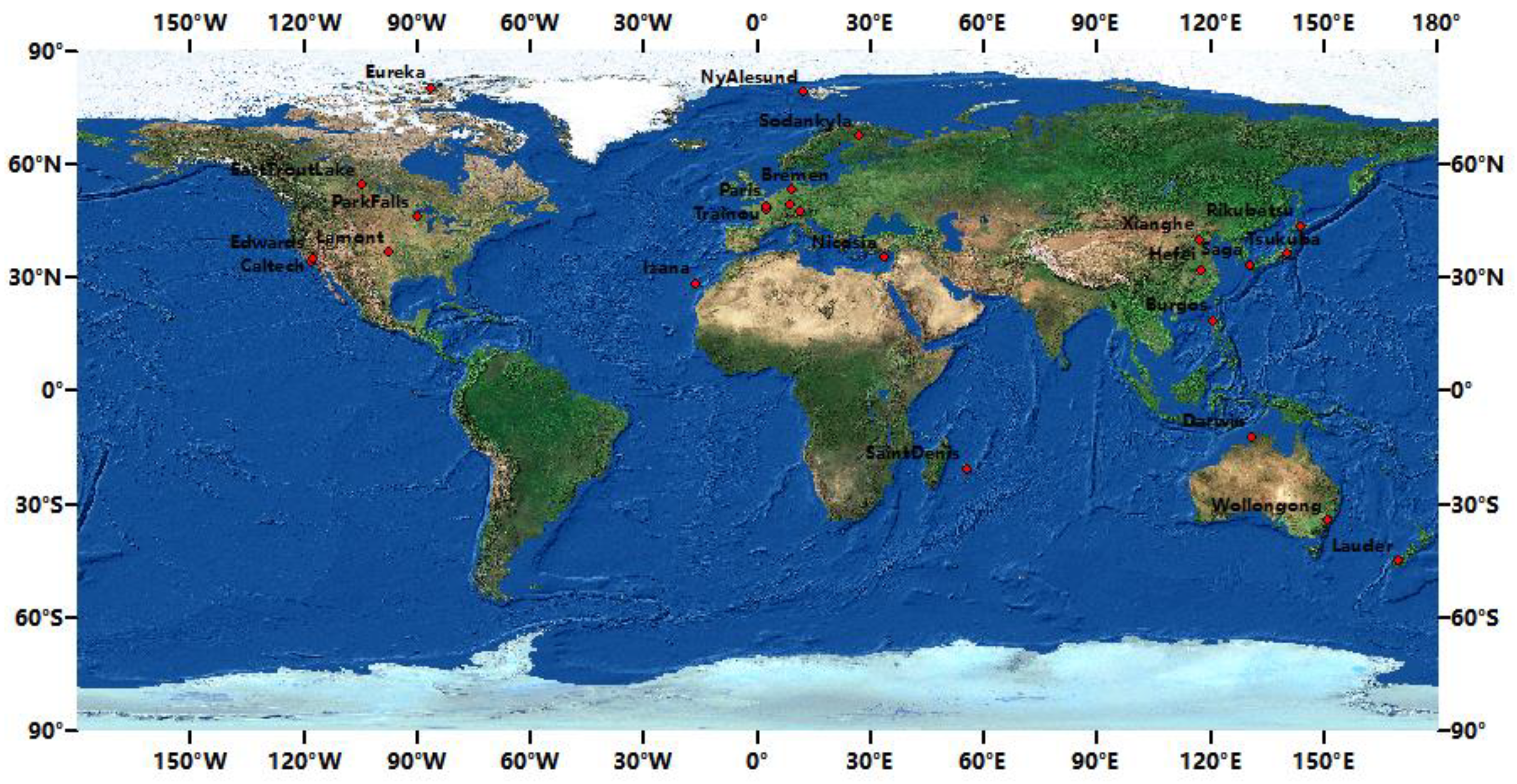
Figure 1. Distribution of TCCON stations.
Atmosphere 15 00118 g001
Figure 2. Technical flowchart.
Atmosphere 15 00118 g002
Figure 3. Correlation and significance heatmap of XCO2 with features (*, **, *** = significant at 0.01, 0.05 and 0.001 probability levels).
Atmosphere 15 00118 g003
Figure 4. The spectral plots of CrIS on 1 January 2019, at the Xianghe (39.8° N, 116.96° E) site.
Atmosphere 15 00118 g004
Figure 5. The R2, RESE, and MAE of the ERT model trained with different features.
Atmosphere 15 00118 g005
Figure 6. XCO2 concentration prediction using a scatter plot of the training set model based on correlation and significance analysis and PCA. (The red dashed line represents the isoproportion line, while the blue dashed line represents the fitted line. The color of the points varies with density.)
Atmosphere 15 00118 g006
Figure 7. Scatter plot of predicted XCO2 concentrations in the validation set. (The red dashed line represents the isoproportion line, while the blue dashed line represents the fitted line. The color of the points varies with density).
Atmosphere 15 00118 g007
Figure 8. The mean and standard deviation of XCO2 observations and model predictions at 12 TCCON sites.
Atmosphere 15 00118 g008
Figure 9. Monthly mean of XCO2 concentration from TCCON observations and model predictions in four major regions: (a) Asia; (b) Europe; (c) North America; (d) Oceania.
Atmosphere 15 00118 g009
Table 1. Information for TCCON stations used for validation.
NameLonLatNumberNameLonLatNumber
Xianghe116.9639.816,075Rikubetsu143.7743.463976
Hefei117.1731.913002SaintDenis26.6367.379825
Zugspitze10.9847.423567Paris2.3648.8521,442
Wollongong150.88−34.4119,508ParkFalls−90.2745.9421,986
Tsukuba140.1236.0513,990Trainou2.1147.9715,753
NyAlesund11.9278.924736Lamont−97.4936.628,766
Lauder169.68−45.0442,984Eureka−86.4280.057652
Karlsruhe8.4449.18229EastTrout−104.9954.3639,992
Saga130.2933.2415,147Edwards−117.8834.9657,555
Izana−16.4828.312,940Darwin130.89−12.4312,838
Garmisch47.4811.068803Caltech−118.1334.1436,000
Bremen8.8553.11451Burgos120.6518.5332,649
Sodankyla26.6367.3713,050Nicosia33.3835.1410,476
Table 2. The specific feature information used in model training.
Variable AbbreviationFull Name of the VariableUnitTemporal ResolutionSpatial ResolutionData Sources
XCO2Column-averaged CO2 dry air mole fractionppmv--TCCON
lonLongitude 6 min50 km × 50 kmCloud-cleared radiances V2
latLatitude
monthMonthm
ddDaysd
bandRadiancemw/(m2 sr cm−1)
szaSolar zenith angle-
saaSolar azimuth angledegree
zaZenith angle-
aaAzimuth angle-
P1 *100 hpahPa1 h0.25° × 0.25°ERA5
T1 *Temperature at 100 hpaK
U1 *U-component of wind at 100 hpam/s
V1 *V-component of wind at 100 hpam/s
W1 *Vertical velocity at 100 hpapa/s
blhBoundary layer heightm
cbhCloud bottom heightm
tpTotal precipitation-
clLake cover-
tccTotal cloud coverage-
sktSkin temperatureK
t2m2 m TemperatureK
tco3Total column ozonekg/m−2
NDVINormalized difference vegetation index-16 d250 m × 250 mMOD13Q1
SRSurface reflectance%1 d500 m × 500 mMOD09GA
DEMDigital elevation modelm--GLOBE Topography
* T, U, V, and W at different vertical air pressures from 100–1000 hPa.
Table 3. Detailed settings of model parameters.
Modeln_EstimatorsMax_DepthMin_Samples_SplitMin_Samples_Leaf
ERT4003051
GBRT3002555
XGBoost 4003080.2
Table 4. The various evaluation metrics of the model training results.
ModelR2RMSE (ppmv)MAE (ppmv)
ERT (PCA)0.92310.75520.5568
ERT (CSA)0.90290.80260.5704
GBRT (PCA)0.90670.79070.5812
GBRT (CSA)0.89380.84580.6163
XGBoost (PCA)0.89950.83820.6371
XGBoost (CSA) 0.87010.93680.6777
Table 5. Validation results of the three models.
ModelR2RMSE (ppmv)MAE (ppmv)
ERT0.90060.79940.5804
GBRT0.87200.90680.6705
XGBoost0.87680.88970.6624
Disclaimer/Publisher’s Note: The statements, opinions and data contained in all publications are solely those of the individual author(s) and contributor(s) and not of MDPI and/or the editor(s). MDPI and/or the editor(s) disclaim responsibility for any injury to people or property resulting from any ideas, methods, instructions or products referred to in the content.