Abstract
This study aimed to investigate the effect of human heart-rate synchronization with variations in the geomagnetic field (GMF) (“biogeophysical synchronization effect”). We analyzed 403 electrocardiogram (ECG) recordings of 100 or 120 min that were obtained in 2012–2023 from two middle-aged female volunteers in good health. The minute-value series of the GMF vector from the INTERMAGNET network was used. Each ECG recording was individually examined using cross-correlation and wavelet analysis. The findings from two separate experimental sets (306 recordings from Volunteer A and 97 from Volunteer B) displayed notable similarity in all aspects analyzed: (1) For both participants, the biogeophysical synchronization effect is observed in 40–53% of the recordings as a statistically significant (p < 0.0045) correlation between minute heart-rate (HR) time-series values and at least one of the horizontal components of the GMF, with a time shift between values of [−5, +5] min. (2) Wavelet analysis indicates that the spectra of the HR series and at least one GMF component exhibit similarity in 58–61% of cases. (3) The synchronization is most evident within the period range between 8–13 min. The probability of the synchronization effect manifestation was independent of the geomagnetic activity (GMA) level, which was recorded during the observations.
1. Introduction
The phenomenon of the human cardiovascular system’s response to variations in space-weather factors has long attracted the attention of researchers.
There are two reasons for this attention: on the one hand, there is the desire to understand the fundamental mechanisms of solar–biospheric interactions.
On the other hand, sudden changes in space weather may prove to be dangerous for individuals with cardiovascular diseases [1,2,3,4,5,6,7,8,9,10,11,12,13,14,15,16,17]. This necessitates a comprehensive analysis of possible risks; which external impacts pose a danger, for whom exactly they are dangerous, and what precautions can be taken. This is the main reason why many heliobiological studies to date have focused on the special aspects of the cardiovascular systems’ reactions.
The following logic can be seen in the development of heliobiological ideas.
The first studies of solar–biosphere relations date back to the 19th century [1]. These were systematized and developed in the works of A.L. Chizhevsky [1,2,3] and mainly concerned the links between changes in solar activity (SA) in a 11-year cycle and the population responses of various large biosystems; for example, the timing of epidemics in different countries.
The following decades, especially those since the 1970s, brought a wealth of research showing that not only the rhythm of the 11-year SA cycles but also short-term (1–3-day long) space-weather phenomena can exert severe, even catastrophic, effects on human health. Solar flares with coronal mass ejections, Forbush decreases, and planetary geomagnetic storms (GMS) were studied in relation to their possible contribution to changes in medical and population indices, such as the number of hypertensive crises, strokes, cases of ischemia, and sudden death. The research studies usually examined large groups of people; for example, the population of a city or region, patients at a particular hospital, etc. [4,5,6,7,8,9,10,11,12,13,14,15,16,17].
Other aspects of solar–biospheric connections were discovered step by step:
- (1)
- In some cases, the strong GMS or abrupt changes in cosmic-ray intensity can have not only a catastrophic but also a reversible biological effect; for example, an increase in blood pressure (without a hypertensive crisis) or other reversible changes in the general condition in groups of individuals [18,19,20,21,22];
- (2)
- Significant deterioration in patient health can be observed not only during major space-weather events, but also during moderate geomagnetic disturbances [23,24,25,26,27,28] and periods of extremely low GMA [29,30,31,32], suggesting that the system of solar–biospheric connections is non-linear and non-monotonic;
- (3)
- The observed biological effects from the GMS of different origins (caused by Corotating Interaction Regions or by the body of Coronal Mass Ejection in interplanetary space [33]) vary significantly [8,34,35]. Therefore, consideration of the origin of GMS is essential for an accurate analysis of potential bioeffects.
- (4)
- The impact of space weather on individuals can vary greatly in terms of time, magnitude, and even direction [36,37]. As a result, a new approach to studying heliobiological effects has emerged that is aimed at analyzing long-term observations of a certain individual [36,37,38,39,40,41,42]. This approach identified the specific trait features of an effect unobserved in group studies.
- (5)
- GMS and other space-weather phenomena affect not only the patients with cardiac disorders but also virtually healthy people [37,38,39,40,41,42,43,44,45,46,47,48,49,50,51].
It can be seen from the above that the development of heliobiological concepts was moving from the examination of large effects of essential space-weather events to their increasingly weaker manifestations. On the other hand, the list of biological responses under examination was gradually expanding, and the catastrophic responses of the body were supplemented with reversible ones at the beginning, and later on, with responses close to the physiological norm. Currently, all of the above approaches remain relevant and are attracting the attention of researchers [32,52,53,54,55,56,57,58,59,60,61,62,63,64,65,66,67,68,69,70,71].
Finally, about ten years ago, a new type of response was discovered, which became the next stage in the study of the heliobiological effect manifestation. In this case, the average value of the measured physiological parameter remains within normal limits. The response is manifested as an adjustment of the body-rhythm frequency to the frequency of the GMF vector variations [72,73,74,75,76,77].
Though the hypotheses on the existence of this mechanism were proposed over half a century ago [78], they were not experimentally validated until recently.
Currently, the effect of biogeophysical synchronization has not yet been sufficiently studied.
The papers that have been published so far either describe measurements that were intentionally performed at low geomagnetic activity (Kp(3h) ≤ 3) [73,79,80] or that did not analyze the possible influence of the GMA level on the effect [74,75].
Therefore, it is unclear to what extent the manifestation of this effect depends on factors such as the level of geomagnetic activity. However, many studies have shown that the phase of the solar-activity cycle or the average GMA level during observations significantly affect the manifestation of the heliobiological effect [13,38,69,81,82].
At the same time, it is reasonable to believe that for a person with heart-rhythm disturbances in a state of rest and relaxation (for example, during sleep), the effect of biogeophysical synchronization can pose a serious danger, because under these conditions, a “capture” or “disruption” of the heart rhythm is potentially possible. It is no coincidence that a sharp deterioration in the well-being of such cardiac patients very often occurs in the early morning when the person is at rest.
For these reasons, examination of the heliobiological manifestation effects at any level is important for both basic and applied purposes; that is, the comprehension of the mechanisms of living systems’ interaction with the environment, and the protection of individuals against the detrimental effects of this interaction.
The objective of this study was to examine the potential correlation between the manifestation of the biogeophysical synchronization effect in healthy individuals and the level of geomagnetic activity.
2. Materials and Methods
2.1. Collection of Experimental Data
Previously, researchers had discovered notable differences in the manifestation of the biogeosynchronization phenomenon among participants [73,74,75,83,84]. To minimize potential errors resulting from individual variability, we implemented a long-term, multiyear experimental design involving two female participants, aged 63 and 54, who lived in the central latitudes of Russia. They were considered to be in good health and susceptible to geomagnetic field variations, as demonstrated by preliminary observations.
The participants were screened for cardiovascular diseases (primarily heart-rhythm disorders), diabetes, and bad health habits. Exclusion criteria included severe fatigue, stress, infectious diseases, and coffee consumption within four hours before measurement.
Measurements were taken at rest in a supine position and in a state of quiet wakefulness. No conversations, sudden movements, or changes in body position were permitted during ECG recordings. Participants were, however, allowed to listen to or watch audio and video files featuring popular science content such as videos exploring animal life or guides to geographical wonders. Such an experimental design was aimed at excluding the influence of sudden external stimuli that could cause abrupt changes to the heart rate or autonomic balance.
Volunteer A conducted 306 ECG recordings, each lasting 100 min, between 2020 and 2022, at the same location in the north of the Moscow region.
Volunteer B conducted 97 recordings, each lasting 120 min, between 2012 and 2023 at various locations, including the Arkhangelsk region, Leningrad region, Moscow region, and Sofia (Bulgaria).
Table 1 shows that all statistical parameters of the participants’ HR were within the physiologically normal range.

Table 1.
Statistical characteristics of volunteers’ heart rates.
A recording duration of 100–120 min provides adequate accuracy for determining the values of present periods within the range of up to 30 min. Additionally, this duration is not sufficiently long to cause significant changes to the body’s condition due to such factors as hunger, thirst, immobility, fatigue, etc.
To record and process the ECG signal, we used technical and software tools developed by Medical Computer Systems LLC. These included the “KARDI-2” unit for recording the ECG signal and a package of application programs known as “CardioVisor-06sI” (Zelenograd).
After each recording, the researcher evaluated the ECG signal to verify the accuracy of automatically detected R-peaks and corrected any potential recognition errors if needed. The RR intervals from each recording were transformed into a time sequence of HR values per minute, consisting of n = 100 or n = 120 points each.
2.2. Geomagnetic Data
One-minute readings of the X and Y components of the GMF vector were chosen as the geophysical indicators based on data collected from geomagnetic stations closest to each measurement point. Thus, the study employed data from Nurmijarvi stations (NUR, 60.500 N, 24.600 E) for the Arkhangelsk region (64°34′ N/40°32′ E), Borok stations (BOX, 58.070 N, 38.230 E) for the Moscow region (55°45′ N/37°36′ E), and St. Petersburg (60°542′ N/29°716′ E) stations for the Leningrad region (59°57′ N/30°19′ E). Additionally, the Panagyurishte station (PAG, 42.50 N, 24.20 E) was used for Sofia (42°40′ N/23°20′ E). Data were obtained from the INTERMAGNET network (https://imag-data.bgs.ac.uk/GIN_V1/GINForms2 accessed on 2 December 2023). Daily values of the Kp index (https://kp.gfz-potsdam.de/en/data, accessed on 2 December 2023) were used to evaluate the planetary GMA level.
We used the X and Y components of the GMF vector because prior research [79] confirmed that their wavelet spectra in the 3–40 min range change quite weakly with distance. The minute-by-minute fluctuations of the GMF Z-component are heavily affected by the underlying surface at the measurement point. Due to this fact, in our testing conditions, the use of data on the dynamics of the GMF Z-component (and, consequently, of the full vector F) is inappropriate.
2.3. Analysis Procedure
Calculations were performed in the MATLAB R2010a software environment using built-in functions and custom applications.
At the preliminary stage, trends and low-frequency fluctuations were excluded from the geophysical and biological time series, which could be due to internal reasons for each process, but, at the same time, these would contribute to the value of the indicators of their statistical relationship.
For this purpose, each 100 min segment of the series was filtered using a bandpass filter with a Blackman–Harris window and values for the lower and upper cut-off frequencies of Fl = 0.02–0.08 and Fr = 0.9995 of the Nyquist frequency, respectively. The lower limit of the filter was selected based on the requirement that the maximum amplitudes in the frequency ranges of 5–20 min and 20–50 min are comparable in magnitude.
Figure 1 displays the effect of the filtering technique on time-series data. For example, the time series of HR values of Volunteer A in two experiments in November 2021 are shown.
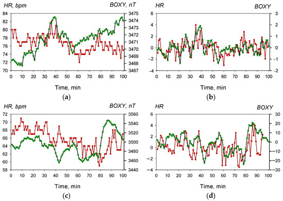
Figure 1.
Examples of changes in the time series after application of a bandpass filter. Red line—the minute HR values of Volunteer A; green line—the synchronous values of the GMF Y-component observed at the Borok geophysical station (BOXY). (a) Experiment 19 November 2021: Time = 11:55 UT; Kp(daily) = 9; Kp (12–15 UT) = 1.7; Dst(d) = 1 nT; original data; (b) Time series from Figure 1a after filtration. (c) Experiment 4 November 2021: Time = 10:17 UT; Kp(daily) = 39.7; Kp(09–12 UT) = 7.7; Dst(d) = −59 nT); original data; (d) Time series from Figure 1c after filtration.
The study involved cross-correlation analysis, wavelet analysis, and a combination of both.
Correlation analysis. First, we computed the Spearman rank-correlation coefficient, which is insensitive to the shape of the sampling distribution. The computation involved 11 different intervals of time lags (−5...5 min) between the HR values and their corresponding X and Y values of the GMF. Then, we screened the 11 resultant correlation coefficients to find the one with the largest modulus coefficient. Its value was used as the correlation value in the experiment. To compensate for the additional degrees of freedom introduced by the inclusion of multiple time-lag values in the analysis, the statistical significance cut-off of p = 0.05 was adjusted according to the Bonferroni correction for 11 degrees of freedom. Correlation coefficients with a significance level of p < 0.0045 were considered statistically significant.
Wavelet analysis. We used the wavelet-transform method with the basic complex Morlet function because it gives good frequency resolution [85].
We used the built-in Matlab “cwt” function: WT = cwt(X) returns the continuous wavelet transform (cwt) of X. If X is real-valued (as is in our case), then WT is a 2-D matrix where each row corresponds to one scale.
In order to facilitate interpretation of the results obtained by the different methods, the scale parameters obtained by wavelet analysis were converted into time characteristics similar to the periods of the oscillations in spectral analyses.
The algorithm for calculating the scalar quantity characterizing the degree of similarity of the wavelet transform spectra included the following steps:
- The wavelet transformation of a 100-point segment of the HR series, within the tested periods of T = 3...50 min, produces a 2-D matrix of wavelet coefficients (W(HR)s) of size i × n, where i ranges from 1 to 50, and n denotes the point number in the data series that corresponds to the experiment’s minutes. It is worth noting that the association between i and T is monotonous but non-linear. Matrices illustrating the HR series (W(HR)) and the GMF vector Y (W(Y)) can be found in Figure 2a,c, respectively. Along the abscissa axis, the experimental time is displayed in minutes, while the T period values are displayed on the ordinate axis. The spectral density of each period is represented by red gradations.
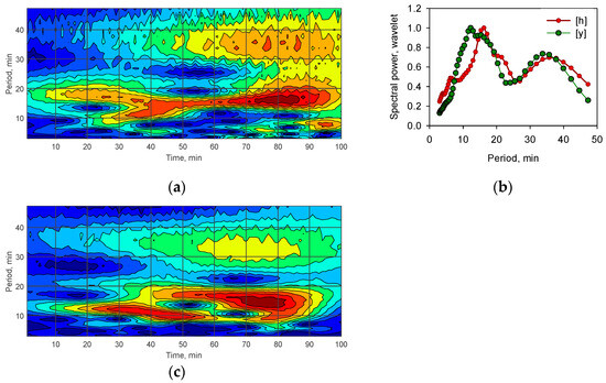 Figure 2. An example of the wavelet transformation of the HR time series of Volunteer A and the GMF vector Y in the 04.11.2021 experiment. (a) Wavelet image of the HR series; (b) Vectors [h] and [y] as a result of averaging wavelet matrices of the HR and BOXY series for each period; (c) Wavelet image of the GMF vector Y.
 - We calculate the arithmetic mean of the values in each row i (i = 1...50) of the wavelet matrix W(HR) and obtain the average values of the amplitudes of each period for n minutes of the experiment (vector [h], size 1 × 50). Then we normalize the vector [h] to its maximum value to facilitate comparison of their shapes. For the series of geomagnetic components X and Y of the GMF vector, we similarly compute the matrices and vectors [x] and [y]. Examples of vectors [h] and [y] are shown in Figure 2b.
- As a scalar quantity characterizing the degree of similarity/difference between the spectra of the HR and Y series, we calculate the values of Qy between a pair of vectors, [h] and [y], as the value of the scalar product of these vectors, normalized to the length of each of them, i.e., Qy = (h,y)/|h|∙|y|.
The calculation of the value Qy is performed not in a space of dimension of 50 (the full dimension of the vectors [h] and [y]) but in a space of dimension m = 32 (for line numbers i = 16...47), which corresponds to the range of periods T = 7...40 min. This exclusion of the smallest (T = 3...6.7 min) and longest periods (T = 40...50 min) when calculating the Qy parameter was made because, in these ranges, there is a decrease in amplitude regardless of the set filter boundaries. Therefore, the incorporation of these ranges in the computation of the Qy value would augment it and also reduce the precision of this numerical indicator with regards to the alignment or non-alignment of peak positions in the time range of 7–40 min. The similarity parameter Qx for wavelet spectra W(HR) and W(X) is calculated in a similar way.
The Qy parameter’s mathematical meaning equates to the cosine of the angle between [h] and [y] or their correlation coefficient, which has values ranging from −1 to 1. However, neighboring values of these vectors are not autonomous; hence, conventional algorithms for measuring statistical significance cannot apply to them. Therefore, we chose the limit of Qx and Qy parameter values that would indicate co-directionality between two vectors and similarity in the corresponding spectra empirically, i.e., at the Qf ≥ 0.4 level. For the situation depicted in Figure 2b, Qy was measured as 0.546.
Combined approach (wavelet analysis and correlation). The purpose of applying this approach was to establish whether there are particular periods that contribute most to the synchronization effect or if this phenomenon affects all oscillation periods within the 3–50 min range equally.
Let j represent the experiment number of Volunteer A, with taking on values of j ranging from 1 to 306. For each experiment j, we complete steps 1–3 outlined in the preceding section: obtaining the wavelet coefficient matrices W(HR)j, W(X)j, and W(Y)j and calculating the average amplitude vectors [h]j, [x]j, and [y]j for each j = 1 through to j = 306.
Now, we establish a 50 × 306 matrix of the G(HR) results from the arrays of vector values [h]j for j = 1, 2,..., 306, where each row j is a vector of values [h]j from the j-th experiment, and each column i is a sequence of amplitudes for period i across all 306 experiments. We also form G(X) and G(Y) matrices in a similar manner using the vectors [x]j and [y]j, respectively.
For each i (i = 1, 2,..., 50), we compute the Spearman correlation coefficients Rx(i) between the j-th (j = 1, 2,..., 306) values in the columns numbered i in the matrices G(HR) and G(X). This coefficient demonstrates the degree to which periods of the same number occur synchronously in the time series of HR and X elements of the GMF vector.
Consecutive experiments of Volunteer A were separated by intervals of at least 20 h, and Volunteer B’s by at least one hour. Within an hour, a person’s heart-rate parameters can vary significantly due to potential movements such as standing up, walking, or talking, so we can consider each ECG recording to be independent from previous and subsequent measurements. Therefore, to assess the synchronicity of the appearance of a certain period in a sequence of experiments, we can use the traditional criterion for assessing the level of statistical significance of the correlation coefficient.
3. Results
Data obtained from each experiment (306 registrations for Volunteer A and 97 for Volunteer B) were processed with the above-described algorithm to calculate the following values:
- The Spearman correlation coefficient of the HR series against the series of each X and Y component of the GMF. Correlation cases were considered significant at p < 0.0045.
- The cosine of angles Qx and Qy between the vectors of averaged amplitudes of wavelet spectra HR [h] and the components of the GMF vectors [x] and [y] (the spectra were deemed similar when values of Qx and Qy exceeded Qf = 0.4).
- Correlation coefficients Rx and Ry between the amplitude values of different periods ranging from 3 to 50 min (based on the full set of experiments for each of the volunteers).
3.1. Results of Cross-Correlation Analysis
Table 2 presents the total number and percentage of experiments conducted with each volunteer, where the correlation coefficients between the HR time series and the X and Y vector time series were statistically significant at p < 0.0045.
Table 2.
The total number and percentage of experiments with a statistically significant correlation.
The sample set of Volunteer A’s results contains 114 cases (37%) of significant correlations for vector X, and 92 cases (30%) for vector Y. Volunteer’s B sample contains 23 (24%) and 20 (21%) such cases, respectively. At the same time, evaluation by the criterion “similarity to at least one of the components of the GMF vector” shows that Volunteer A’s sample set contains 163 such cases (58%), while Volunteer B’s contains 39 (i.e., 40%).
To evaluate whether the level of GMA has an impact on the probability of a synchronization effect occurrence, we have distributed the results of each volunteer into four samples according to the Kp-index values on the day of measurements (Kp-daily), with the limits for the GMA levels detailed in Table 3.
Table 3.
Limits of Kp-index values and the number of trials for different GMA levels.
Setting boundaries for each GMA level enabled the acquisition of four comparable sample sizes of experiments for each volunteer, corresponding to different levels. Table 3 displays the observed range of Kp values from completely calm days to middle magnetic storms for both volunteers.
Figure 3 shows the percentage distribution of cases that display a significant correlation (p < 0.0045) according to the GMA level for Volunteers A and B.
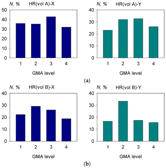
Figure 3.
Relative frequency of cases with a statistically significant correlation between the HR series and the GMF vector component based on the GMA level (a) for Volunteer A and (b) for Volunteer B.
According to the χ2-test, there were no statistically significant (p < 0.05) differences between any two bars within each of the four distributions presented in Figure 3.
3.2. The Findings of the Wavelet Spectra Similarity Analysis
Table 4 displays the absolute and relative number of experiments for each volunteer where the wavelet spectra of the HR series were found to be similar to the spectra of the X and Y vector series at the Qf = 0.4 similarity-threshold value.
Table 4.
Absolute and relative numbers of cases with similarities between the wavelet spectra of HR and GMF.
Table 4 shows that the proportion of spectra found to be similar in both volunteers and for both GMF components appears to be very close, both when assessed by a single GMF component (41–43%) and by their combination (58–61%).
Figure 4 presents the relative values of Qx and Qy for three threshold levels: Qf = 0.3, 0.4, and 0.5. The value of Qf = 0.4 was chosen as the threshold value for cases of close bio- and geo-wavelet spectra. The stability of the relative magnitudes of the bars belonging to different GMA levels was additionally assessed by testing the threshold values of 0.3 and 0.5.
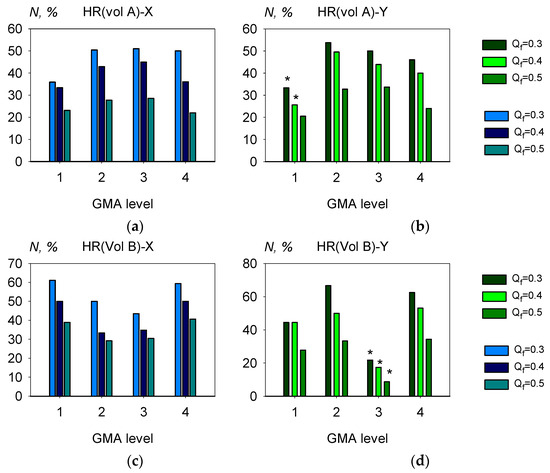
Figure 4.
Relative number of Qx and Qy values exceeding the Qf threshold at the three levels of Qf = 0.3, 0.4, 0.5 for Volunteer A (a,b) and for Volunteer B (c,d). *—statistically significant cases (p < 0.05). See text below for detailed explanation.
In the case of Volunteer A, the only statistically significant (p < 0.05) case of pairwise differences relates to the distribution of component Y (Figure 4b): the value for GMA level 1 differs from the values for levels 2 and 3 at the threshold values of Qf = 0.3 and 0.4. Similarly, for Volunteer B (Figure 4d), the value for level 3 is significantly different from those for levels 2 and 4 at all three Qf threshold values.
These two statistically significant (p < 0.05) cases have different trends: in the first case (Figure 4b), the percentage of similar spectra at the lowest GMA level is lower than at the three higher ones. In the second case (Figure 4d), the minimum percentage is observed at level 3 of the GMA. In addition, in all tested cases, no significant differences between levels 1 and 4 were found. Thus, it can be inferred that significant deviations in these cases may occur randomly, and the likelihood of similarity between the spectra of the HR series and the GMF vector is not influenced by the overall level of geomagnetic perturbation.
3.3. Analysis of the Synchronous Occurrence of Matching Cycles in Biological and Geomagnetic Series
Figure 5 shows the results of analyzing the synchrony of the occurrence of oscillations of equal frequencies in the HR series and X and Y components of the GMA vector for the whole set of individual experiments for Volunteers A (Figure 5a) and B (Figure 5b). The horizontal red line indicates the p = 0.05 statistical significance level of the correlation coefficient, given the experimental sample size for each volunteer.
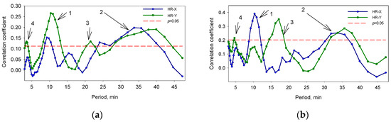
Figure 5.
Correlation coefficients of coincident period amplitude values in successive experiments (a) for Volunteer A and (b) for Volunteer B. Arrows 1-4 indicate periods where the correlation coefficient is p < 0.05. See text below for detailed explanation.
Comparison of Figure 5a and 5b shows two ranges of oscillations with approximately the same boundaries and with a significance level of p > 0.05 that are present in both graphs:
- (1)
- 8.3–13.0 min (maximum 10.3 min) for Volunteer A and 9.2–11.6 min (maximum 10.3 min) for Volunteer B;
- (2)
- A group of periods ranging from 25 to 40 min for Volunteer A and from 30 to 40 min for Volunteer B.There are also two groups of statistically significant periods whose boundaries are different in Figure 5a,b:
- (3)
- 15.3–18.2 min for Volunteer B; however, in Figure 5a, there is only a small peak corresponding to 20 min.
- (4)
To clarify the degree of stability of the observed periods, we divided the whole set of experiments for each volunteer into 4 subsets according to the value of Kp-daily, like in Section 3.1 and Section 3.2 (Table 3).
The results of the analysis are presented in Figure 6. The red dashed line shows the significance level of p = 0.05, considering the number of experiments falling into this subset.
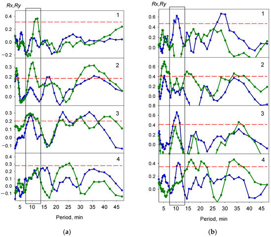
Figure 6.
Correlation coefficients Rs between the values of the amplitudes of the same periods in successive experiments for Volunteer A (a) and Volunteer B (b) at different levels of GMA (1–4; top to bottom). Blue line—Rx; green line—Ry; red dashed—p = 0.05.
The vertical rectangle in both figures highlights the 8–13 min periods ranges. It can be seen that for Volunteer A at Kp-index levels 1, 2 and 3 and for Volunteer B at levels 1, 3, and 4, a statistically significant period falls within this range. Thus, in both cases, in three of the four distributions, a synchronous occurrence of this range period can be observed in the biological rhythm and variations of the GMF vector.
Periods of 30–40 min show statistical significance in two samples for Volunteer A (at levels 2 and 3) and in three samples for Volunteer B (at levels 2, 3, and 4). The other ranges display high variability, especially for Volunteer B, due to the decreased statistical values of each sample during the process of subset selection.
- The oscillation period in the range of 8–13 min occurs in the HR spectra of volunteers simultaneously, with its occurrence in the spectrum of at least one of the GMF vector components. With somewhat less certainty, we can say the same about periods of 30–40 min.
- Like the case of Section 3.1 and Section 3.2, we cannot observe any difference in the extent of this effect at different GMA levels.
- The other cases of correlation, even significant ones, in some samples of the experiment should, for now, be considered noise effects that require further verification due to their unstable manifestation.
4. Discussion
4.1. Independence of the Synchronization Effect from the GMA Level
The results of all three applied methods of analysis indicate that the probability of occurrence of the biogeophysical synchronization effect remains approximately the same, regardless of the average GMA level during the observation period. The fact that this result was obtained independently for two large non-overlapping experimental samples further increases the level of its validity.
An analysis of a very large array of heliobiological results over the past 25 years has shown [82] that at different levels of functioning of a complex system of solar–biosphere connections, the influence of space-weather factors on biological objects can manifest itself in various forms. This is a property of the system itself and not a consequence of errors in experiments.
For an accurate comparison of various heliobiological results, it is important to select only those that most closely match our experimental design based on at least three criteria: First, the level of the biological system under examination; for example, a population, a group of individuals, a whole body, a body system, a separate organ, a cell, an organelle, or perhaps a separate biomolecule. Second, the data sampling frequency (years, months, days, minutes, seconds). And finally, third, the amplitude (or nature) of the observed biological response: (1) irreversible response (death or disease); (2) adaptive response (i.e., reversible but with a significant change in the average value of the physiological indicator); (3) response without a change in the average value, which is expressed in a change in frequency rather than amplitude.
We studied the behavior of HR indices, which are very popular in heliobiological studies. However, almost all studies of HR relate either to daily and monthly time scales or to the assessment of group average or medical population indices (such as disease complications or mortality) [13,37,39,43,44,48,50,51]. The overall conclusion from this large body of results is that GMS and other significant space-weather events lead to changes in the values of many physiological indicators that reflect the cardiovascular system condition (we call this the “first type of effect”).
According to the three criteria described above, the biogeosynchronization effect (the “second type of effect”) differs from the first type in two aspects. The first of them is the form of the effect manifestation. In all the studies mentioned above, the observed effect is a change in the average HR value (“irreversible response” or “adaptive response with a reversible shift in the mean value”); in the second case, only its spectral indicators change (“response without a shift in the mean value”). When studying the first type of effect, it is possible to evaluate such reaction parameters as the moment of its beginning, its duration, and its amplitude. In the second case, such estimates are not applicable.
The second difference is the disparate time scales. The first effect was traditionally observed on a daily data-sampling scale (in some cases, even the next day). The effect of biogeophysical synchronization was observed at a minute-data collection rate, and the processes under study were characterized by much shorter development times. When averaging them by the 24 h time interval, we may observe only a very slow envelope of these processes.
Therefore, it can be assumed that the change in mean HR caused by the GMF and the synchronization effect are separate but complementary aspects of the solar–biosphere relationship. The synchronization effect may or may not be observed at the minute scale, while a change in the mean HR value caused by the GMF may or may not be detected on a daily basis, even in the same individual. Further research is necessary to establish a comprehensive phenomenological and biophysical framework linking these two phenomena.
At the same time, there are few works that examine HR and GMF vector variations using a minute-data sampling rate and applying an individual approach to data analysis. The studies conducted by Timofeeva et al. [74,75] and Poskotinova et al. [77] are the most relevant to our experimental design. Timofeeva et al. demonstrated the synchronization of human HR with GMF vector variations using different computational methods than ours. Poskotinova et al. investigated the frequency of synchronization effects in groups of healthy individuals and in those with arterial hypertension. However, similar to our previous studies [79,80], none of these works considered the impact of the GMA level on the synchronization effect.
Furthermore, the division of GMAs based on the Kp-index value, which has already been implemented, can be assumed to be suitable for the first stage of the analysis. However, it is necessary to clarify in the future the possible dependence of the synchronization effect on the surrounding geomagnetic environment. To accomplish this, it is necessary to analyze the existing measurement results by categorizing them according to the origin of the observed magnetic storms and the different phases of the storm (sudden onset, main phase, and recovery phase).
4.2. Possible Scheme of the “Rhythm Capture” Process
Our findings reveal that not all periods from the studied frequency range contribute equally to the “rhythm capture” process. Synchronization is most evident in the frequency range of 8–13 min, with a peak at 10 min. Fluctuations at this frequency appear in the HR precisely in these recordings where this period is discernible in the GMF component spectrum.
These conclusions fit well into the following possible scheme of the development of the synchronization process:
- Stable oscillations occur in the GMF spectrum, with a period close to 10 min (ranging from 8 to 13 min);
- These oscillations cause a “rhythm capture” of a physiological process in the human organism, which has its own oscillation period within this range and which, in turn, can influence the cardiac rhythmicity;
- Hence, the mentioned physiological process’s contribution to the establishment of cardiac rhythmicity is amplified, resulting in the manifestation of the 10 min oscillation period in the heart-rhythm spectrum.
The frequency range at 8–13 min stands out from the other parts of the examined range due to the specific characteristics of the effect. It is worth noting that the synchronization effect displaying stability at varying levels of GMA was also observed within the range at 25–40 min. In addition, we observed the manifestation of the effect at other periods (Figure 2), where the main power of the spectrum is concentrated in the periods at 15–18 min and about 35 min. At the same time, the power at the 10 min period is much lower, although the period can be found in both spectra. Thus, the 8–13 min range can be recognized as very interesting and promising for further study, but it is clearly not unique.
Additionally, Poskotinova et al. [77] indirectly confirmed this finding. In their study, as the left limit of the filter was shifted toward high frequencies, more subjects showed a correlation between heart-rate variability (HRV) parameters and variations in the GMF vector.
Periods of 7 min, 13 min, and 25–30 min were observed in the spectra of minute values of the stable nitric oxide metabolite NOx, which were close to both the period of the HR and the period of the spectra of synchronous changes in the GMF vector [80]. It is also known that the change in vascular sensitivity to nitric oxide is a link mediating the baroreflex response to magnetic storms in rabbits [86].
Other studies [83,84] have found that, among the tested HRV parameters, the spectral measures of low-frequency HRV show the strongest correlation with magnetic vector variations.
These data indicate a need to increase the frequency of data sampling in further studies and to expand the list of physiological parameters to include HRV indices.
The authors of [74,75,77] come to conclusion that the ability of a person’s HR to synchronize with the GMF rhythm in the millihertz range can be considered a positive property of the body, indicating its good health [74,75] and good adaptive reserves [77]. In [74,75], the most pronounced synchronization effect was observed in a large number of healthy individuals when they were in a calm and positive state. In [77], the synchronization effect was observed more often in healthy people than in patients with high blood pressure, and its decrease was associated with a decrease in baroreflex sensitivity.
Our experimental design aimed to minimize any sudden external stimuli that could affect the HR and autonomic balance, but we did not consider the general psycho-emotional state of the volunteers during the measurements. Therefore, this should be taken into account in further studies.
Of the significant space-weather effects that have already been studied, predominantly negative consequences have been shown for organisms (death, disease, and deterioration of well-being). Based on current knowledge, the biogeosynchronization effect appears to be neutral. It is more commonly observed in individuals who are in a good psycho-emotional and physical state. However, it is important to note that this effect has not been studied in individuals with arrhythmias, ischemic heart disease, or other cardiological disorders.
The authors of [87] found that the lowest rate of acute admissions to the Psychiatric Inpatient Unit of the University of Crete corresponds to the period when the highest number of large (M > 6.4) and moderate (M > 4.5) earthquakes (EQs) in the geographic region was observed. On the contrary, the maximum number of value admissions was recorded in the month of August 2010 in the absence of large EQs but a greater number of (small) EQs.
According to their hypothesis, the increases/decreases in the admission of patients to a psychiatric unit are related to two different kinds of seismic activity and, associated with these, different amplitude-frequency portraits of the surrounding electromagnetic environment. They suggest that certain combinations of very low-frequency electromagnetic field characteristics, characteristic of periods of large earthquakes, may have a “positive”, i.e., “therapeutic” effect on the mental state of people.
It may be appropriate to consider this hypothesis when examining the impact of space weather on the human cardiovascular system, including the effect of biogeosynchronization. This could lead to new developments in our understanding of solar–biospheric relationships.
5. Conclusions
This paper presents an analysis of the association between the heart-rate dynamics of healthy individuals and synchronous variations in the horizontal components of the geomagnetic field. The study analyzed multiyear monitoring data from two female volunteers in good health (306 and 97 records, respectively).
The experimental design minimized potential interference from individual variations in the effect as well as from any subjects’ actions that could affect their heart rate, such as talking, moving, or external emotional stimuli.
The conclusions for each participant were obtained individually, and they demonstrated almost identical results in all aspects evaluated.
The biogeophysical synchronization effect has two manifestations: the correlation between minute HR values and variations in the GMF, and the coincidence of the main periods of oscillations within the 3–50 min range.
The synchronization process is not evenly distributed throughout the entire range of oscillations, but is predominantly present at period ranges of around 10 min (8–13 min) and 25–40 min. All the above instances of the synchronization effect are not influenced by the GMA level during the observations.
The absence of a correlation between the level of GMA and the probability of effect manifestation does not contradict prior findings on the alteration of HRV indices values during magnetic storms. Instead, it highlights yet another dimension of the solar–biospheric relationship. It is feasible this phenomenon serves as a rhythm sensor for a healthy organism under normal circumstances. There is reason to believe that the likelihood of an effect appearing is contingent on a person’s physiological and/or psycho-emotional state; however, this requires additional investigation.
Author Contributions
Conceptualization, T.A.Z. and T.K.B.; methodology, T.A.Z.; software, T.A.Z.; validation, T.A.Z. and N.I.K.; formal analysis, T.A.Z.; investigation, N.I.K.; resources, T.A.Z. and N.I.K.; data curation, N.I.K.; writing—original draft preparation, review, and editing, T.A.Z. and T.K.B.; visualization, T.A.Z.; project administration, T.K.B. All authors have read and agreed to the published version of the manuscript.
Funding
The work was carried out according to the state task of ITEB RAS (state registration № 075-01025-23-01) and the state task “Plazma” of IKI RAS.
Institutional Review Board Statement
The study was conducted in accordance with the Declaration of Helsinki and approved by the Ethics Committee Institute of Theoretical and Experimental Biophysics, Russian Academy of Sciences (protocol code 06/2012 from 01.06.2012).
Informed Consent Statement
Informed consent was obtained from all subjects involved in the study. Written informed consent has been obtained from the patients to publish this paper.
Data Availability Statement
Geomagnetic field one-minute data used in this study are openly available in INTERMAGNET—British Geological Survey network (https://imag-data.bgs.ac.uk/GIN_V1/GINForms2 accessed on 2 December 2023). Daily values of the Kp index are openly available in GFZ German Research Centre for Geosciences (https://kp.gfz-potsdam.de/en/data, accessed on 2 December 2023). Heart-rate recording database is not publicly available due to privacy and ethical reasons.
Acknowledgments
The results presented in this paper rely on data collected at magnetic observatories. We thank the national institutes that support them and INTERMAGNET for promoting high standards of magnetic observatory practices (https://imag-data.bgs.ac.uk/GIN/ accessed on 2 December 2023).
Conflicts of Interest
The authors declare no conflicts of interest.
References
- Chizhevsky, A.L. The Terrestrial Echo of Solar Storms; Mysl: Moscow, Russia, 1976; p. 366. (In Russian) [Google Scholar]
- Chijevsky, A.L. The correlation between the variation of sun-spot activity and the rise and spreading of epidemils. Rapport le 17 octobre 1930. In Proceedings of the XIII Congresso International de Hidrologia, Climatologia e Geologia Medicas, Programa des Sessoes Scientificas, 2 Sessao, Lisboa, Portugal, 1930. [Google Scholar]
- Chijevsky, A.-L. Les Epidemies et Les Perturbations Electromagnetiques Du Milieu Exterieur; Depot General Le Francois: Paris, France, 1938. [Google Scholar]
- Gnevyshev, M.N.; Novikova, K.F.; Ohl, A.I.; Tokareva, N.V. Sudden death from cardiovascular diseases and solar activity. In Influence of Solar Activity on the Atmosphere and Biosphere of the Earth; Nauka: Moscow, Russia, 1971; pp. 179–187. (In Russian) [Google Scholar]
- Villoresi, G.; Breus, T.K.; Iucci, N.; Dorman, L.I.; Rapoport, S.I. The influence of geophysical and social effects on the incidences of clinically important pathologies (Moscow, 1979–1981). Phys. Medica 1994, 10, 79–91. [Google Scholar]
- Villoresi, G.; Breus, T.K.; Dorman, L.I.; Iuchi, N. Effect of interplanetary and geomagnetic disturbances on the increase in number of clinically serious medical pathologies (myocardial infarct and stroke). Biofizika 1995, 40, 983–993. [Google Scholar]
- Baevsky, R.M.; Petrov, V.M.; Cornelissen, G.; Halberg, F.; Orth-Gomer, K.; Akerstedt, T.; Otsuka, K.; Breus, T.; Siegelova, J.; Dusek, J.; et al. Meta-analyzed heart rate variability, exposure to geomagnetic storms, and the risk of ischemic heart disease. Scr. Med. 1997, 70, 11543511. [Google Scholar]
- Villoresi, G.; Ptitsyna, N.G.; Tiasto, M.I.; Iucci, N. Myocardial infarct and geomagnetic disturbances: Analysis of data on morbidity and mortality. Biofizika 1998, 43, 623–631. [Google Scholar] [PubMed]
- Gurfinkel’, I.; Kuleshova, V.P.; Oraevskiĭ, V.N. Assessment of the effect of a geomagnetic storm on the frequency of appearance of acute cardiovascular pathology. Biofizika 1998, 43, 654–658. (In Russian) [Google Scholar] [PubMed]
- Halberg, F.; Cornelissen, G.; Otsuka, K.; Watanabe, Y.; Katinas, G.S.; Burioka, N.; Delyukov, A.; Gorgo, Y.; Zhao, Z.; Weydahl, A.; et al. Cross-spectrally coherent ~10,5- and 21-year biological and physical cycles, magnetic storms and myocardial infarctions. Neuroendocrinol. Lett. 2000, 21, 233–258. [Google Scholar] [PubMed]
- Dorman, L.I.; Iucci, N.; Ptitsyna, N.G.; Villoresi, G. Cosmic rays as indicator of space weather influence on frequency of infract myocardial, brain strokes, car and train accidents. In Proceedings of the 27th International Cosmic Ray Conference, Hamburg, Germany, 7–15 August 2001; p. 3511. [Google Scholar]
- Stoupel, E.; Domarkiene, S.; Radisauskas, R.; Abramson, E. Sudden cardiac death and geomagnetic activity: Links to age, gender and agony time. J. Basic Clin. Physiol. Pharmacol. 2002, 13, 11–22. [Google Scholar] [CrossRef]
- Cornelissen, G.; Halberg, F.; Breus, T.; Syitkina, E.; Baevsky, R.; Weydahl, A.; Watanabe, Y.; Otsuka, K.; Siegelova, J.; Fiser, B.; et al. Non-photic solar assotiations of heart rate variability and myocardial infarction. J. Atmos. Sol. Terr. Phys. 2002, 64, 707–720. [Google Scholar] [CrossRef]
- Wickramasinghe, N.C. Is the 2019 novel coronavirus related to a spike of cosmic rays? Adv. Genet. 2020, 106, 119–122. [Google Scholar] [CrossRef]
- Stoupel, E.; Kalediene, R.; Petrauskiene, J.; Starkuviene, S.; Abramson, E.; Israelevich, P.; Sulkes, J. Clinical Cosmobiology: Distribution of Deaths during 180 Months and Cosmo Physical Activity. The Lithuanian Study, 1990–2004. In The Role of Cosmic Rays. Study Report; Division of Cardiology Rabin Medical Center Tel Aviv University: Tel Aviv, Israel, 2004. [Google Scholar]
- Díaz-Sandoval, R.; Erdélyi, R.; Maheswaran, R. Could periodic patterns in human mortality be sensitive to solar activity? Ann. Geophys. 2011, 29, 1113–1120. [Google Scholar] [CrossRef]
- Feigin, V.L.; Parmar, P.G.; Barker-Collo, S.; Bennett, D.A.; Anderson, C.S.; Thrift, A.G.; Stegmayr, B.; Rothwell, P.M.; Giroud, M.; Bejot, Y.; et al. Geomagnetic Storms Can Trigger Stroke: Evidence from 6 large population-based studies in Europe and Australasia. Stroke 2014, 45, 1639–1645. [Google Scholar] [CrossRef] [PubMed]
- Ghione, S.; Mezzasalma, L.; Del Seppia, C.; Papi, F. Do geomagnetic disturbances of solar origin affect arterial blood pressure? J. Hum. Hypertens. 1998, 12, 749–754. [Google Scholar] [CrossRef] [PubMed]
- Dimitrova, S.; Stoilova, I.; Cholakov, I. Influence of local geomagnetic storms on arterial blood pressure. Bioelectromagnetics 2004, 25, 408–414. [Google Scholar] [CrossRef] [PubMed]
- Dimitrova, S.; Mustafa, F.R.; Stoilova, I.; Babayev, E.S.; Kazimov, E.A. Possible influence of solar extreme events and related geomagnetic disturbances on human cardio-vascular state: Results of collaborative Bulgarian–Azerbaijani studies. Adv. Space Res. 2009, 43, 641–648. [Google Scholar] [CrossRef]
- Azcárate, T.; Mendoza, B.; Levi, J.R. Influence of geomagnetic activity and atmospheric pressure on human arterial pressure during the solar cycle 24. Adv. Space Res. 2016, 58, 2116–2125. [Google Scholar] [CrossRef]
- Galata, E.; Ioannidou, S.; Papailiou, M.; Mavromichalaki, H.; Paravolidakis, K.; Kouremeti, M.; Trachanas, K. Impact of space weather on human heart rate during the years 2011–2013. Astrophys. Space Sci. 2017, 362, 138. [Google Scholar] [CrossRef]
- Rodriquez-Taboada, E.R.; Sierra-Figueredo, P.; Figueredo, S.S. Geomagnetic activity related to acute myocardial infarctions: Relationship in a reduced population and time interval. Geofis. Int. 2004, 43, 265–269. [Google Scholar] [CrossRef]
- Kleimenova, N.; Kozyreva, O.; Breus, T.; Rapoport, S. Pc1 geomagnetic pulsations as a potential hazard of the myocardial infarction. J. Atmos. Sol.-Terr. Phys. 2007, 69, 1759–1764. [Google Scholar] [CrossRef]
- Giannaropoulou, E.; Papailiou, M.; Mavromichalaki, H.; Gigolashvili, M.; Tvildiani, L.; Janashia, K.; Preka-Papadema, P.; Papadima, T. A study on the various types of arrhythmias in relation to the polarity reversal of the solar magnetic field. Nat. Hazards 2014, 70, 1575–1587. [Google Scholar] [CrossRef]
- Ziubryte, G.; Siauciunaite, V.; Jarusevicius, G.; McCraty, R. Local earth magnetic field and ischemic heart disease: Peculiarities of interconnection. Cardiovasc. Disord. Med. 2018, 3, 1–3. [Google Scholar] [CrossRef]
- Fdez-Arroyabe, P.; Fornieles-Callejón, J.; Santurtún, A.; Szangolies, L.; Donner, R.V. Schumann resonance and cardiovascular hospital admission in the area of Granada, Spain: An event coincidence analysis approach. Sci. Total Environ. 2020, 705, 135813. [Google Scholar] [CrossRef] [PubMed]
- Shaposhnikov, D.; Revich, B.; Gurfinkel, Y.; Naumova, E. The influence of meteorological and geomagnetic factors on acute myocardial infarction and brain stroke in Moscow, Russia. Int. J. Biometeorol. 2013, 58, 799–808. [Google Scholar] [CrossRef] [PubMed]
- Stoupel, E. Effect of geomagnetic activity on cardiovascular parameters. J. Clin. Basic Cardiol. 1999, 2, 34–40. [Google Scholar] [CrossRef] [PubMed]
- Stoupel, E.; Babayev, E.S.; Abramson, E.; Sulkes, J. Days of “Zero” level geomagnetic activity accompanied by the high neutron activity and dynamics of some medical events—Antipodes to geomagnetic storms. Health 2013, 5, 855–861. [Google Scholar] [CrossRef]
- Stoupel, E.; Richardas, R.; Vidmantas, V.; Gailute, B.; Abdonas, T.; Evgeny, A. Data about Natural History of Some Acute Coronary Events at Days of High Cosmic Ray (CRA)-Neutron Activity and Following 48 Hours (2000–2012). Health 2016, 8, 402–408. [Google Scholar] [CrossRef]
- Vencloviene, J.; Radisauskas, R.; Tamosiunas, A.; Luksiene, D.; Sileikiene, L.; Milinaviciene, E.; Rastenyte, D. Possible Associations between Space Weather and the Incidence of Stroke. Atmosphere 2021, 12, 334. [Google Scholar] [CrossRef]
- Borovsky, J.E.; Denton, M.H. Differences between CME-driven storms and CIR-driven storms. J. Geophys. Res. Space Phys. 2006, 111, A07S08. [Google Scholar] [CrossRef]
- Breus, T.K.; Baevskii, R.M.; Nikulina, G.A.; Chibisov, S.M.; Chernikova, A.G.; Pukhlianko, M.; Oraevskii, V.N.; Halberg, F.; Cornelissen, G.; Petrov, V.M. Effect of geomagnetic activity on the human body in extreme conditions and correlation with data from laboratory observations. Biofizika 1998, 43, 811–818. (In Russian) [Google Scholar]
- Dimitrova, S.; Stoilova, I.; Georgieva, K.; Taseva, T.; Jordanova, M.; Maslarov, D. Solar and geomagnetic activity and acute myocardial infarction morbidity and mortality. Fundam. Space Res. Supl. Compt. Rend. Acad. Bulg. Sci. 2009, 161–165. [Google Scholar]
- Shepoval’nikov, V.N.; Soroko, S.I. Human Meteo Sensitivity; Ilim: Bishkek, Kyrgyzstan, 1992; p. 247. (In Russian) [Google Scholar]
- Chernouss, S.; Vinogradov, A.; Vlassova, E. Geophysical Hazard for Human Health in the Circumpolar Auroral Belt: Evidence of a Relationship between Heart Rate Variation and Electromagnetic Disturbances. Nat. Hazards 2001, 23, 121–135. [Google Scholar] [CrossRef]
- Watanabe, Y.; Cornélissen, G.; Halberg, F.; Otsuka, K.; Ohkawa, S.I. Associations by signatures and coherences between the human circulation and helio- and geomagnetic activity. Biomed. Pharmacother. 2000, 55, 76–83. [Google Scholar] [CrossRef] [PubMed]
- Otsuka, K.; Yamanaka, T.; Cornelissen, G.; Breus, T.; Chibisov, S.M.; Baevsky, R.; Siegelova, J.; Fiser, B.; Halberg, F. Altered chronome of heart rate variability during span of high magnetic activity. Scr. Med. 2000, 2, 113–118. [Google Scholar]
- Poskotinova, L.V.; Grigoriev, P.E. The Dependence of Typological Autonomic Features Reactions of Healthy Persons on Background Helio-Meteofactors. Hum. Ecol. 2008, 5, 3–8. (In Russian) [Google Scholar]
- Zenchenko, T.A.; Dimitrova, S.; Stoilova, I.; Breus, T.K. Individual types of blood pressure reactions of practically healthy people to the effect of geomagnetic activity. Clin. Med. 2009, 4, 18–23. (In Russian) [Google Scholar]
- Wanliss, J.; Cornélissen, G.; Halberg, F.; Brown, D.; Washington, B. Superposed epoch analysis of physiological fluctuations: Possible space weather connections. Int. J. Biometeorol. 2017, 62, 449–457. [Google Scholar] [CrossRef] [PubMed]
- Otsuka, K.; Cornélissen, G.; Weydahl, A.; Holmeslet, B.; Hansen, T.; Shinagawa, M.; Kubo, Y.; Nishimura, Y.; Omori, K.; Yano, S.; et al. Geomagnetic disturbance associated with decrease in heart rate variability in a subarctic area. Biomed. Pharmacother. 2000, 55, 51–56. [Google Scholar] [CrossRef]
- Oinuma, S.; Kubo, Y.; Otsuka, K.; Yamanaka, T.; Murakami, S.; Matsuoka, O.; Ohkawa, S.; Cornélissen, G.; Weydahl, A.; Holmeslet, B.; et al. Graded response of heart rate variability, associated with an alteration of geomagnetic activity in a subarctic area. Biomed. Pharmacother. 2002, 56, 284–288. [Google Scholar] [CrossRef] [PubMed]
- Mitsutake, G.; Otsuka, K.; Hayakawa, M.; Sekiguchi, M.; Cornelissen, G.; Halberg, F. Does Schumann resonance affect our blood pressure? Biomed. Pharmacother. 2005, 59, S10–S14. [Google Scholar] [CrossRef]
- Papailiou, M.; Kudela, K.; Stetiarova, J.; Giannaropoulou, E.; Mavromichalaki, H.; Dimitrova, S. The effect of cosmic ray intensity variations and geomagnetic disturbances on the physiological state of aviators. Astrophys. Space Sci. Trans. 2011, 7, 373–377. [Google Scholar] [CrossRef]
- Breus, T.; Baevskii, R.; Chernikova, A. Effects of geomagnetic disturbances on humans functional state in space flight. J. Biomed. Sci. Eng. 2012, 5, 341–355. [Google Scholar] [CrossRef]
- Mavromichalaki, H.; Papailiou, M.; Dimitrova, S.; Babayev, E.S.; Loucas, P. Space weather hazards and their impact on human cardio-health state parameters on Earth. Nat. Hazards 2012, 64, 1447–1459. [Google Scholar] [CrossRef]
- Azcárate, T.; Mendoza, B.; De La Peña, S.S.; Martínez, J. Temporal variation of the arterial pressure in healthy young people and its relation to geomagnetic activity in Mexico. Adv. Space Res. 2012, 50, 1310–1315. [Google Scholar] [CrossRef]
- Dimitrova, S.; Angelov, I.; Petrova, E. Solar and geomagnetic activity effects on heart rate variability. Nat. Hazards 2013, 69, 25–37. [Google Scholar] [CrossRef]
- Ozheredov, V.A.; Chibisov, S.M.; Blagonravov, M.L.; Khodorovich, N.A.; Demurov, E.A.; Goryachev, V.A.; Kharlitskaya, E.V.; Eremina, I.S.; Meladze, Z.A. Influence of geomagnetic activity and earth weather changes on heart rate and blood pressure in young and healthy population. Int. J. Biometeorol. 2017, 61, 921–929. [Google Scholar] [CrossRef]
- Vaičiulis, V.; Radišauskas, R.; Ustinavičienė, R.; Kalinienė, G.; Tamošiūnas, A. Associations of morbidity and mortality from coronary heart disease with heliogeophysical factors. Environ. Sci. Pollut. Res. 2016, 23, 18630–18638. [Google Scholar] [CrossRef]
- Vencloviene, J.; Antanaitiene, J.; Babarskiene, R. The association between space weather conditions and emergency hospital admissions for myocardial infarction during different stages of Solar activity. J. Atmos. Sol. Terr. Phys. 2016, 149, 52–58. [Google Scholar] [CrossRef]
- Caswell, J.M.; Carniello, T.N.; Murugan, N.J. Annual incidence of mortality related to hypertensive disease in Canada and associations with heliophysical parameters. Int. J. Biometeorol. 2016, 60, 9–20. [Google Scholar] [CrossRef]
- Vencloviene, J.; Babarskiene, R.M.; Kiznys, D. A possible association between space weather conditions and the risk of acute coronary syndrome in patients with diabetes and the metabolic syndrome. Int. J. Biometeorol. 2017, 61, 159–167. [Google Scholar] [CrossRef]
- Mavromichalaki, H.; Preka-Papadema, P.; Theodoropoulou, A.; Paouris, E.; Apostolou, T. A study of the possible relation of the cardiac arrhythmias occurrence to the polarity reversal of the solar magnetic field. Adv. Space Res. 2017, 59, 366–378. [Google Scholar] [CrossRef]
- Gurfinkel, Y.I.; Vasin, A.L.; Pishchalnikov, R.Y.; Sarimov, R.M.; Sasonko, M.L.; Matveeva, T.A. Geomagnetic storm under laboratory conditions: Randomized experiment. Int. J. Biometeorol. 2018, 62, 501–512. [Google Scholar] [CrossRef]
- Gurfinkel, Y.I.; Ozheredov, V.A.; Breus, T.K.; Sasonko, M.L. The Effects of Space and Terrestrial Weather Factors on Arterial Stiffness and Endothelial Function in Humans. Biophysics 2018, 63, 299–306. [Google Scholar] [CrossRef]
- Podolská, K. The impact of ionospheric and geomagnetic changes on mortality from diseases of the circulatory system. J. Stroke Cerebrovasc. Dis. 2018, 27, 404–417. [Google Scholar] [CrossRef]
- Vencloviene, J.; Braziene, A.; Dobozinskas, P. Short-Term Changes in Weather and Space Weather Conditions and Emergency Ambulance Calls for Elevated Arterial Blood Pressure. Atmosphere 2018, 9, 114. [Google Scholar] [CrossRef]
- Vieira, C.L.Z.; Janot-Pacheco, E.; Lage, C.; Pacini, A.; Koutrakis, P.; Cury, P.R.; Shaodan, H.; Pereira, L.A.; Saldiva, P.H.N. Long-term association between the intensity of cosmic rays and mortality rates in the city of Sao Paulo. Environ. Res. Lett. 2018, 13, 24009. [Google Scholar] [CrossRef]
- Pishchalnikov, R.Y.; Gurfinkel, Y.I.; Sarimov, R.M.; Vasin, A.L.; Sasonko, M.L.; Matveeva, T.A.; Binhi, V.N.; Baranov, M.V. Cardiovascular response as a marker of environmental stress caused by variations in geomagnetic field and local weather. Biomed. Signal Process. Control 2019, 51, 401–410. [Google Scholar] [CrossRef]
- Vieira, C.L.Z.; Alvares, D.; Blomberg, A.; Schwartz, J.; Coull, B.; Huang, S.; Koutrakis, P. Geomagnetic disturbances driven by solar activity enhance total and cardiovascular mortality risk in 263 U.S. cities. Environ. Health 2019, 18, 1–10. [Google Scholar] [CrossRef]
- Sasonko, M.L.; Ozheredov, V.A.; Breus, T.K.; Ishkov, V.N.; Klochikhina, O.A.; Gurfinkel, Y.I. Combined influence of the local atmosphere conditions and space weather on three parameters of 24-h electrocardiogram monitoring. Int. J. Biometeorol. 2019, 63, 93–105. [Google Scholar] [CrossRef]
- Kiznys, D.; Vencloviene, J.; Milvidaitė, I. The associations of geomagnetic storms, fast solar wind, and stream interaction regions with cardiovascular characteristic in patients with acute coronary syndrome. Life Sci. Space Res. 2020, 25, 1–8. [Google Scholar] [CrossRef]
- Vencloviene, J.; Radisauskas, R.; Vaiciulis, V.; Kiznys, D.; Bernotiene, G.; Kranciukaite-Butylkiniene, D.; Tamosiunas, A. Associations between Quasi-biennial Oscillation phase, solar wind, geomagnetic activity, and the incidence of acute myocardial infarction. Int. J. Biometeorol. 2020, 64, 1207–1220. [Google Scholar] [CrossRef]
- Vaičiulis, V.; Venclovienė, J.; Tamošiūnas, A.; Kiznys, D.; Lukšienė, D.; Krančiukaitė-Butylkinienė, D.; Radišauskas, R. Associations between Space Weather Events and the Incidence of Acute Myocardial Infarction and Deaths from Ischemic Heart Disease. Atmosphere 2021, 12, 306. [Google Scholar] [CrossRef]
- Mavromichalaki, H.; Papailiou, M.-C.; Gerontidou, M.; Dimitrova, S.; Kudela, K. Human Physiological Parameters Related to Solar and Geomagnetic Disturbances: Data from Different Geographic Regions. Atmosphere 2021, 12, 1613. [Google Scholar] [CrossRef]
- Podolská, K. Circulatory and Nervous Diseases Mortality Patterns—Comparison of Geomagnetic Storms and Quiet Periods. Atmosphere 2022, 13, 13. [Google Scholar] [CrossRef]
- Papailiou, M.; Ioannidou, S.; Tezari, A.; Lingri, D.; Konstantaki, M.; Mavromichalaki, H.; Dimitrova, S. Space weather phenomena on heart rate: A study in the Greek region. Int. J. Biometeorol. 2023, 67, 37–45. [Google Scholar] [CrossRef] [PubMed]
- Qammar, N.W.; Petronaitis, D.; Jokimaitis, A.; Ragulskis, M.; Smalinskas, V.; Žiubrytė, G.; Jaruševičius, G.; Vainoras, A.; McCraty, R. Long Observation Window Reveals the Relationship between the Local Earth Magnetic Field and Acute Myocardial Infarction. Atmosphere 2023, 14, 1234. [Google Scholar] [CrossRef]
- Pobachenko, S.V.; Kolesnik, A.G.; Borodin, A.S.; Kalyuzhin, V.V. The contingency of parameters of human encephalograms and Schumann resonance electromagnetic fields revealed in monitoring studies. Biophysics 2006, 51, 480–483. [Google Scholar] [CrossRef]
- Zenchenko, T.A.; Medvedeva, A.A.; Khorseva, N.I.; Breus, T.K. Synchronization of human heart-rate indicators and geomagnetic field variations in the frequency range of 0.5–3.0 mHz. Izv. Atmos. Ocean. Phys. 2014, 50, 736–744. [Google Scholar] [CrossRef]
- Timofejeva, I.; McCraty, R.; Atkinson, M.; Joffe, R.; Vainoras, A.; Alabdulgader, A.; Ragulskis, M. Identification of a Group’s Physiological Synchronization with Earth’s Magnetic Field. Int. J. Environ. Res. Public Health 2017, 14, 998. [Google Scholar] [CrossRef]
- Timofejeva, I.; McCraty, R.; Atkinson, M.; Alabdulgader, A.A.; Vainoras, A.; Landauskas, M.; Šiaučiūnaitė, V.; Ragulskis, M. Global Study of Human Heart Rhythm Synchronization with the Earth’s Time Varying Magnetic Field. Appl. Sci. 2021, 11, 2935. [Google Scholar] [CrossRef]
- Alabdulgader, A.; McCraty, R.; Atkinson, M.; Dobyns, Y.; Vainoras, A.; Ragulskis, M.; Stolc, V. Long-Term Study of Heart Rate Variability Responses to Changes in the Solar and Geomagnetic Environment. Sci. Rep. 2018, 8, 2663. [Google Scholar] [CrossRef]
- Poskotinova, L.; Krivonogova, E.; Demin, D.; Zenchenko, T. Differences in the Sensitivity of the Baroreflex of Heart Rate Regulation to Local Geomagnetic Field Variations in Normotensive and Hypertensive Humans. Life 2022, 12, 1102. [Google Scholar] [CrossRef]
- Presman, A.S. Electromagnetic Field and Wildlife; Nauka: Moscow, Russia, 1968; 310p. [Google Scholar]
- Zenchenko, T.A.; Jordanova, M.; Poskotinova, L.V.; Medvedeva, A.A.; Alenikova, A.E.; Khorseva, N.I. Synchronization between human heart rate dynamics and Pc5 geomagnetic pulsations at different latitudes. Biophysics 2014, 59, 965–972. [Google Scholar] [CrossRef]
- Zenchenko, T.A.; Medvedeva, A.A.; Potolitsyna, N.N.; Parshukova, O.I.; Boiko, E.R. Correlation of the dynamics of minute-scale heart rate oscillations and biochemical parameters of the blood in healthy subjects to Pc5–6 geomagnetic pulsations. Biophysics 2015, 60, 309–316. [Google Scholar] [CrossRef]
- Zeng, W.; Liang, X.; Wan, C.; Wang, Y.; Jiang, Z.; Cheng, Z.; Cornélissen, G.; Halberg, F.; Wang, Z. Patterns of mortality from cardiac-cerebral vascular disease and influences from the cosmos. Biol. Rhythm. Res. 2014, 45, 579–589. [Google Scholar] [CrossRef]
- Zenchenko, T.A.; Breus, T.K. The Possible Effect of Space Weather Factors on Various Physiological Systems of the Human Organism. Atmosphere 2021, 12, 346. [Google Scholar] [CrossRef]
- Alabdulgade, A.; Maccraty, R.; Atkinson, M.; Vainoras, A.; Berškienė, K.; Mauricienė, V.; Navickas, Z.; Šmidtaitė, R.; Landauskas, M.; Daunoravičienė, A. Human heart rhythm sensitivity to earth local magnetic field fluctuations. J. Vibroeng. 2015, 17, 3271–3278. [Google Scholar]
- McCraty, R.; Atkinson, M.; Stolc, V.; Alabdulgader, A.A.; Vainoras, A.; Ragulskis, M. Synchronization of Human Autonomic Nervous System Rhythms with Geomagnetic Activity in Human Subjects. Int. J. Environ. Res. Public Health 2017, 14, 770. [Google Scholar] [CrossRef]
- Smolentsev, N.K. Fundamentals of wavelet theory. In Wavelets in MATLAB; DMK Press: Moscow, Russia, 2009; p. 448. [Google Scholar]
- Gmitrov, J. Baroreceptor stimulation enhanced nitric oxide vasodilator responsiveness, a new aspect of baroreflex physiology. Microvasc. Res. 2015, 98, 139–144. [Google Scholar] [CrossRef]
- Anagnostopoulos, G.; Basta, M.; Stefanakis, Z.; Vassiliadis, V.; Vgontzas, A.; Rigas, A.; Koutsomitros, S.; Baloyannis, S.; Papadopoulos, G. A study of correlation between seismicity and mental health: Crete, 2008–2010. Geomat. Nat. Hazards Risk 2013, 6, 45–75. [Google Scholar] [CrossRef]


Disclaimer/Publisher’s Note: The statements, opinions and data contained in all publications are solely those of the individual author(s) and contributor(s) and not of MDPI and/or the editor(s). MDPI and/or the editor(s) disclaim responsibility for any injury to people or property resulting from any ideas, methods, instructions or products referred to in the content. |
© 2024 by the authors. Licensee MDPI, Basel, Switzerland. This article is an open access article distributed under the terms and conditions of the Creative Commons Attribution (CC BY) license (https://creativecommons.org/licenses/by/4.0/).