A Sensitivity Study of a Bayesian Inversion Model Used to Estimate Emissions of Synthetic Greenhouse Gases at the European Scale

Abstract

To address and mitigate the environmental impacts of synthetic greenhouse gases it’s crucial to quantify their emissions to the atmosphere on different spatial scales. Atmospheric Inverse modelling is becoming a widely used method to provide observation-based estimates of greenhouse gas emissions with the potential to provide an independent verification tool for national emission inventories. A sensitivity study of the FLEXINVERT+ model for the optimisation of the spatial and temporal emissions of long-lived greenhouse gases at the regional-to-country scale is presented. A test compound HFC-134a, the most widely used refrigerant in mobile air conditioning systems, has been used to evaluate its European emissions in 2011 to be compared with a previous study. Sensitivity tests on driving factors like—observation selection criteria, prior data, background mixing ratios, and station selection—assessed the model’s performance in replicating measurements, reducing uncertainties, and estimating country-specific emissions. Across all experiments, good prior (0.5–0.8) and improved posterior (0.6–0.9) correlations were achieved, emphasizing the reduced sensitivity of the inversion setup to different a priori information and the determining role of observations in constraining the emissions.The posterior results were found to be very sensitive to background mixing ratios, with even slight increases in the baseline leading to significant decrease of emissions.

1. Introduction

Anthropogenic Greenhouse Gas (GHG) emissions have been identified as a pivotal driver of global warming [1], a phenomenon that has far-reaching consequences for our planet’s climate and ecosystems. The human-induced escalation in GHG emissions intensifies the natural greenhouse effect, leading to higher global temperatures and widespread changes in the climate system. A collective effort is needed to limit global warming and its catastrophic consequences. The 2015 Paris Agreement, established under the United Nations Framework Convention on Climate Change (UNFCCC), is a landmark international accord that sets ambitious goals to combat climate change. It aims at strengthening the global response to the threat of climate change, holding the increase in global average temperature to well below 2 degrees Celsius above pre-industrial levels while pursuing efforts to limit the rise to 1.5 degrees Celsius. The mitigation of GHG emissions is crucial for reaching these goals. In this frame, the Paris Agreement calls upon nations to submit nationally determined contributions (NDCs) to reduce their GHG emissions. This includes requirements that all Parties report regularly on their emissions and implementation efforts. National Inventory Reports (NIRs) are detailed reports submitted by UNFCCC parties to report their national GHG emissions and removals. These reports are typically submitted annually and provide a transparent and comprehensive account of a country’s emissions. NIRs must follow specific reporting guidelines and methodologies established by the IPCC (Intergovernmental Panel on Climate Change) [2]. They are built on the so-called bottom-up approach, where emission factors (EFs), which represent the amount of GHG released per unit of activity or source, are multiplied by activity data, which provide information on the level of activity or processes generating emissions (e.g., vehicle miles driven, livestock populations, forest management practices). An alternative approach to estimating emissions is the top-down one, which combines atmospheric observation with transport models that relate emissions to the concentration measured and then deduce the intensity and location of sources. The emissions can be determined using an inversion algorithm that adjusts the emissions used in the model to optimise the agreement between observed and simulated concentration [3]. Several inversion systems are available and have been developed in the past, based on different inversion techniques and atmospheric transport models; all these systems have their strengths and weaknesses that researchers have addressed and optimized to target specific case studies; these systems have been used for different compounds, both natural and anthropogenic, at different temporal and spatial resolution scale, for different observing systems (both ground and satellite base) [4,5,6,7,8,9,10]. Among those gases whose emissions must be reported to UNFCCC, fluorinated gases (F-gases) are the ideal candidates for a top-down verification because they have virtually no natural source interference in the atmospheric measurements, there are considerable uncertainties in inventory methods, they are long-lived, and the loss mechanisms are well known. These synthetic compounds, including hydrofluorocarbons (HFCs), perfluorocarbons (PFCs), and sulfur hexafluoride (SF6), are potent GHGs with extremely high Global Warming Potentials (GWPs), meaning they have much greater heat-trapping effect per molecule than carbon dioxide. By mitigating F-gases, we can significantly lower the anthropogenic contribution to global warming [11]. In the past decade, thanks to the increased capability of producing high-quality atmospheric datasets and to the rapid development of inverse modelling techniques, meaningful progress has been made in the use of atmospheric measurements for estimating F-gas emissions from the global to the regional scale [12,13,14,15,16,17,18,19,20]. Such studies have been used to verify existing inventories [21] and detect unreported emissions [22]. High-quality, high temporal resolution continuous measurements of F-gases in Europe are available at sites that are part of the AGAGE (Advanced Global Atmospheric Gases Experiment network), a global collaborative effort involving multiple research institutions and monitoring stations around the world [23]. The findings of the European AGAGE network help inform policymakers, regulatory bodies, and international agreements such as the Kigali Amendment to the UNEP (United Nations Environment Programme) Montreal Protocol, which seeks to phase down high-GWP F-gases and the European F-gas regulation [24], a comprehensive policy framework aimed at reducing the use and emissions of high-GWP F-gases within the European Union.

This study aims to get an insight into the Bayesian inversion model FLEXINVERT+, focusing on the role of input data and model parameters. FLEXINVERT+ is a recent evolution of the FLEXINVERT model, developed by Thompson and Stohl [25], mainly used for estimating CH₄ fluxes but also applied for the evaluation of others tracers like Black Carbon (BC) [26,27], nitrous oxide (N₂O) [8]. More recently, it has been applied to F-gases to estimate their emissions in Southeast Asia [19]. In light of the foreseen systematic use of FLEXINVERT+ to estimate emissions of F-gases at the European scale, we aimed at optimising the FLEXINVERT+ parameters according to the specific characteristics of this class of compounds and of the domain considered (e.g., the presence of mountain receptors, the relevance of coastal areas, etc.). We used as test compound 1,1,1,2-tetrafluoroethane (HFC-134a), the most emitted HFC, having been used as the primary substitute for the ozone-depleting CFC-12 as a refrigerant in mobile air conditioning (MAC) systems. We compare our results to those obtained by Brunner et al. [16], who presented a comparison among four inverse modelling systems to estimate CO2-eq European emissions of two HFCs (HFC-134a and HFC-125) and SF6 in 2011 and related them with the official inventories submitted by the single countries to the UNFCCC.The rationale for selecting this particular study for comparison, despite its use of a 2011 dataset, lies in its rarity as one of the few studies employing very similar inversion modelling setups. Additionally, the inclusion of an ensemble comprising four distinct inversion setups in this paper provides us with the opportunity to compare our results comprehensively across all these modelling configurations.

2. Materials and Methods

2.1. Inversion Modelling

In this work we used a Bayesian inversion framework, namely FLEXINVERT+, to estimate the surface atmospheric fluxes of HFC-134a. FLEXINVERT+ is an atmospheric inversion system based on the minimization of the cost function defined as:

$$J\left(x\right)=\frac{1}{2}{(p-p_0)}^T{\mathit{B}}^{-1}(p-p_0)+\frac{1}{2}{(Hp-y)}^T{\mathit{R}}^{-1}(Hp-y)$$

(1)

where p and $p_0$ are the optimized and the prior state vector, respectively; y is the mixing ratio enhancements with respect to the background mixing ratios, H is the atmospheric transport function, B is the prior error covariance matrix, and R is the observation error covariance matrix. A detailed description of FLEXINVERT+ is given by Thompson et al. [25]. The components of the atmospheric inversion framework, i.e., observations, a priori emissions field, footprint/emission sensitivity maps, and background mixing ratios, are discussed further.

2.1.1. Observations

The European AGAGE network comprises multiple atmospheric measurement stations located in different countries across Europe. These stations collect air samples and continuously monitor the mixing ratios of F-gases and other GHGs in the atmosphere through a gas chromatographic-mass spectrometric instrumentation, which provides high-precision measurements of multiple species. Having as term of reference the results reported by Brunner et al. [16], we used the 2011 time series from three European AGAGE stations: Monte Cimone (CMN; northern Apennines, Italy), Jungfraujoch (JFJ; Swiss Alps, Switzerland) and Mace Head (MHD; west coast, Republic of Ireland). The geographical configuration of the station allows for describing both substantial regional-scale pollution in the air that has travelled from the populated and industrial regions of Europe and clean westerly air that has travelled across the North Atlantic Ocean. All AGAGE sites rely upon well-defined internal absolute gravimetric calibration procedures that can be repeated periodically to ensure the accuracy of the long-term measured trends. AGAGE implements rigorous QA/QC procedures to ensure that the data collected at its measurement stations are of high quality and can be relied upon for scientific research. Details on the measurement techniques, calibration, and QA/QC procedures are reported by Prinn et al. [23]. Any measurement is associated with uncertainties that are the result of (a) the accuracy of the primary calibration scale originating from the production of the primary standards, (b) the uncertainty from the propagation of the calibration standards within the AGAGE chain from primary to tertiary tank [28], and (c) from tertiary to quaternary (working) tank and real sample calibration [23]; and (d) the precision of the measurements. Measurement precision is derived from the standard deviation of the pairs of working standard measurements that bracket the actual air measurements on a daily basis. While uncertainties listed in (a) and (b) are common for the whole network and are almost well established, values for (c) and (d) are site/instrument specific and may vary with time. For the HFC-134a 2011 dataset, average total uncertainties are in the range of 2.1 to 3% for all the stations used in this study (at two standard deviation levels,

Table 1. HFC-134a measurement uncertainty at three sites.

Station	Primary Scale Accuracy (%)	Scale Propagation Uncertainty	Precision	Average Total Uncertainty (2σ%)
CMN	1	0.7%/0.48 ppt	0.6%–0.44 ppt	3.0
JFJ	1	0.3%/0.16 ppt	0.3%–0.22 ppt	2.2
MHD	1	0.2%/0.15 ppt	0.3%–0.22 ppt	2.1

).

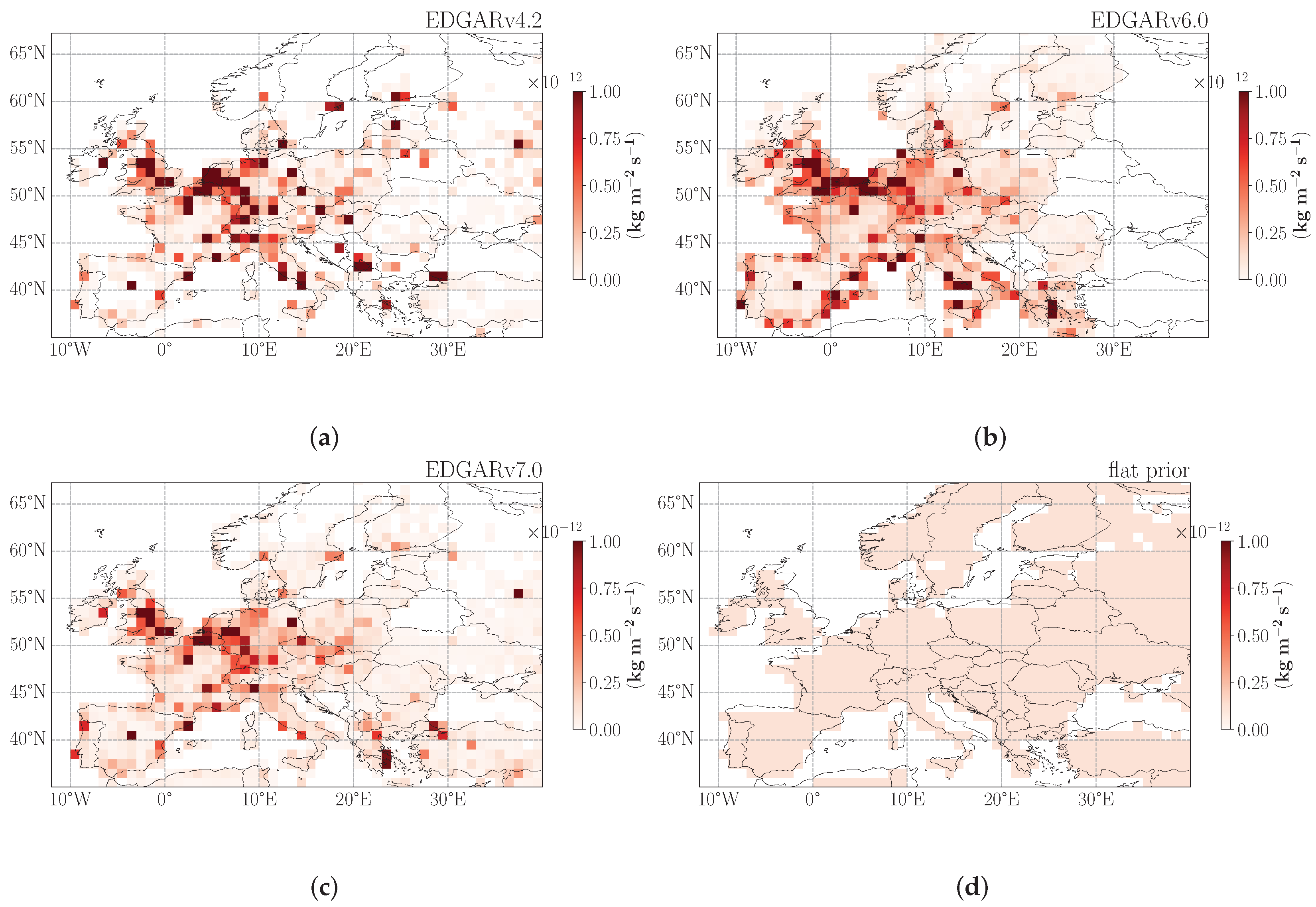
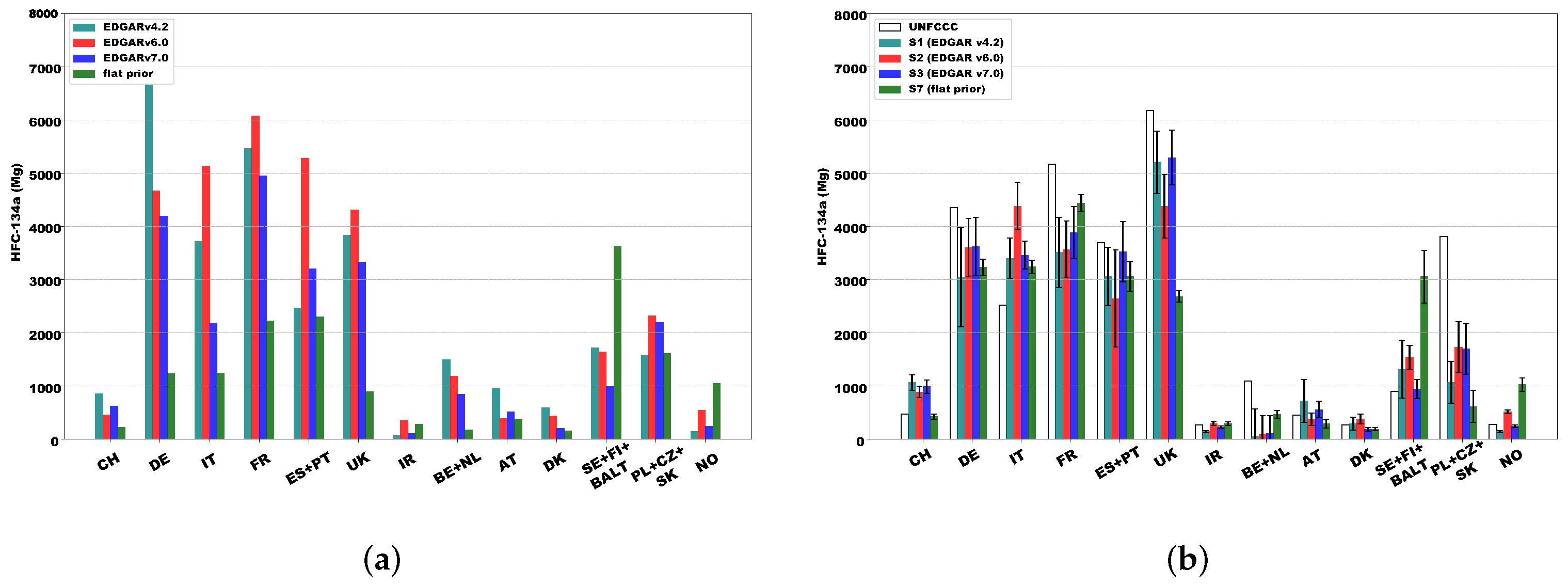
2.1.2. A Priori Emission Field

The bottom-up estimates provided by the Emissions Database for Global Atmospheric Research (EDGAR) are used as a priori information in this study. EDGAR is a global database of anthropogenic emissions of GHGs and air pollutants. It provides global past and present-day independent emission estimates compared to those reported by European Member States or parties under the UNFCCC. The bottom-up estimates are calculated using the emission factors and activity data. They are usually spread over the spatial grid using proxies like the location of energy and manufacturing facilities, road networks, shipping routes, human and animal population density, agricultural land use, etc. We have employed three different EDGAR datasets, namely, EDGAR v4.2, EDGAR v6.0, and EDGAR v7.0 [29,30,31]. The EDGAR v4.2 and EDGAR v7.0 emissions are provided on the spatial resolution grid of 0.1° × 0.1°. The inversion grid used for the inversions is 1° × 1°, so the EDGAR emissions were re-gridded to match the inversion grid resolution. Only EDGAR v6.0 reports the national net emissions: we used population density as a proxy to spread the national net emissions in the respective country at a resolution of 1° × 1°. An additional sensitivity test is performed by flattening the prior information. We spread the total European emissions from the EDGARv7.0 dataset evenly over the land to make a flat prior distribution. Figure 1 represents the four a priori fields used in the inversions.

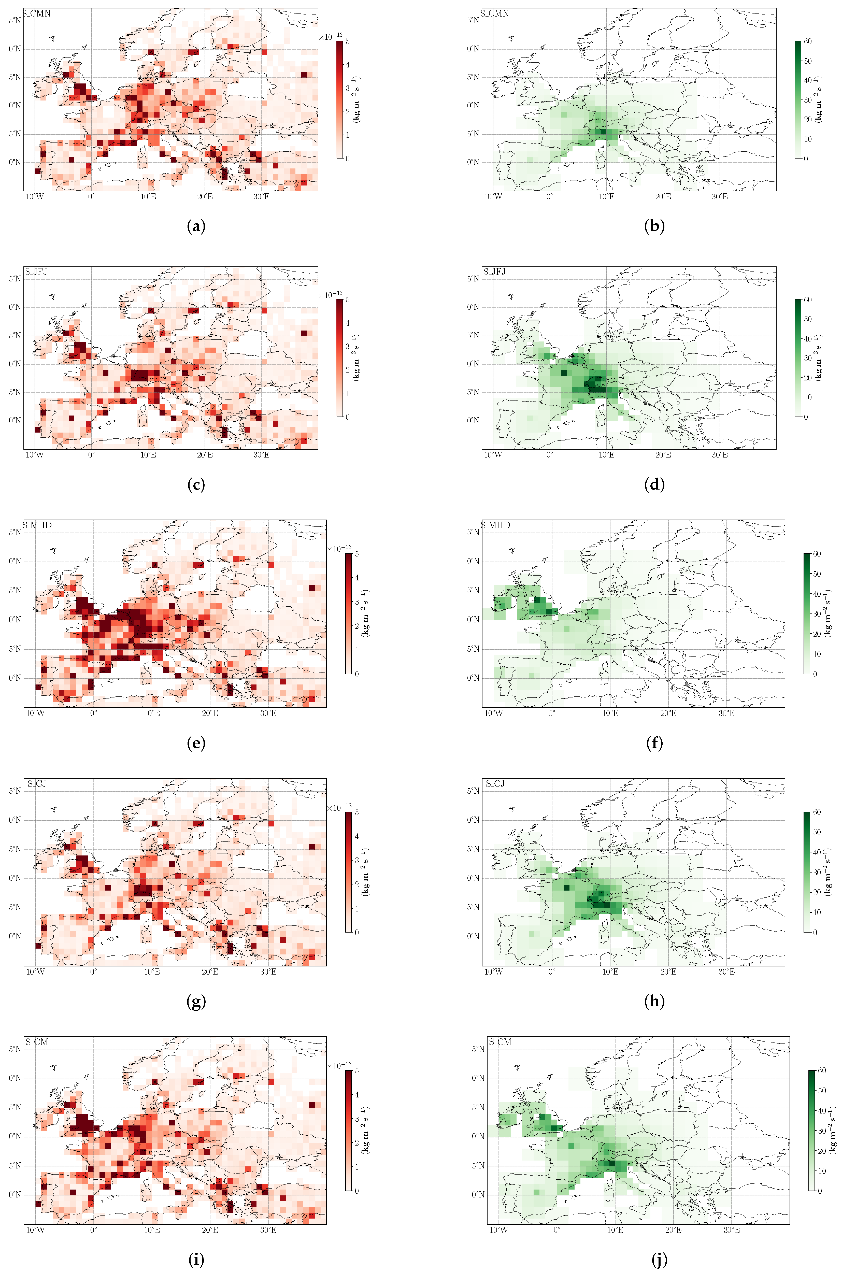
2.1.3. Footprint/Emission Sensitivity Maps

The transport operator, H, represents the source-receptor relationship (SRR) and relates the change in mixing ratio of an atmospheric species to its fluxes. It is also called footprint or emission sensitivity. In this study, we used a Lagrangian Particle Dispersion Model (LPDM) FLEXPART [32] to compute the H operator. In the FLEXPART model, ensembles of particles are released from each receptor site and their trajectories are followed backward in time. The transport of these particles is driven by meteorological fields provided by the European Centre for Medium-Range Weather Forecasts (ECMWF) reanalysis. The SRR is the average residence time of the back trajectories in the grid cell of the source under consideration [33]. FLEXPART has been extensively used in different applications [34,35,36] among others to evaluate the probability of source locations.

In this study, the meteorological data driving the FLEXPART model is obtained from the ERA5 dataset, a fifth-generation ECMWF reanalysis for global climate and weather [37,38]. ERA5 offers both high-resolution reanalysis (HRES) and reduced-resolution ten-member ensemble (EDA) data. The HRES data has a horizontal resolution of 31 km (0.28125°) and 137 hybrid sigma/pressure (model) levels vertically, with the top level at 0.01 hPa. For this study, we have obtained and pre-processed the HRES data at 3-hourly temporal resolution using the open-source software package Flex_extract v7.1.2 [39].

The geographical domain used in the transport model encompasses Europe, with the following boundaries: NW (−30°, 79.78°); NE (42°, 79.78°); SW (−30°, 30°); SE (42°, 30°). At each measurement time, we released 10,000 particles over a 15-minute period. These released particles were tracked backward in time for a duration of 5 days. The release heights for particles at each receptor site are detailed in

Table 2. Setup for FLEXPART simulations.

Parameter	Value/Remarks
Horizontal resolution of the meteorological fields	0.28° × 0.28°
temporal resolution of the meteorological fields	3 h
Horizontal resolution of simulation domain	1° × 1°
Backwards trajectories lengths	5 days
Receptor release height at CMN	2000 m
Receptor release height at JFJ	3000 m
Receptor release height at MHD	26 m

. In mountainous regions, adjustments were made to the release heights to account for the model’s lower orography representation, which is a consequence of the adopted low spatial resolution of 1°.

All the specifications related to the FLEXPART model are mentioned in the Table 2. Figure 2a presents the total sensitivity, displayed on a logarithmic scale, calculated for the year 2011. This total sensitivity is the cumulative sum of the sensitivity values for all receptors and all releases throughout the year.

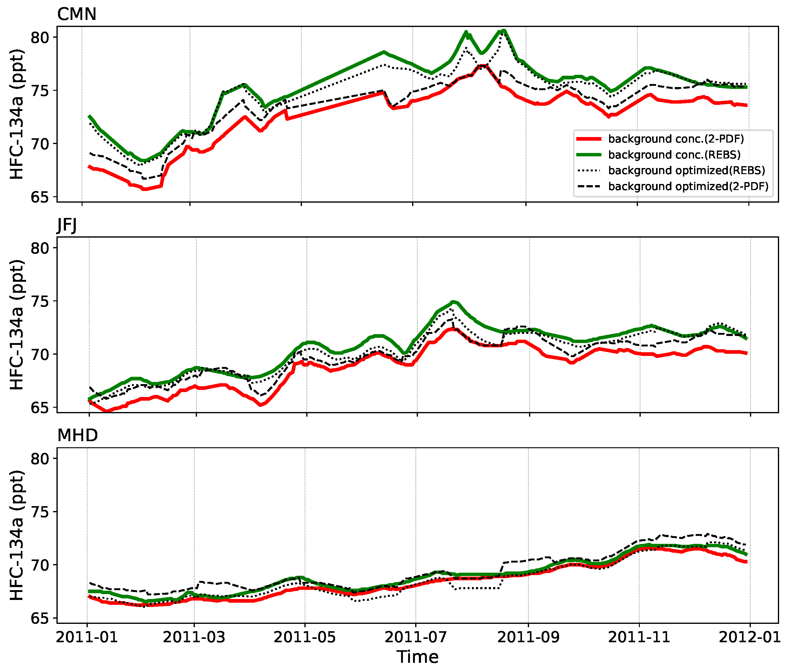
2.1.4. Background Mixing Ratios

The observed variability in mixing ratios results from a combination of factors, including spatial and temporal changes in emissions, meteorological fluctuations, and chemical interactions (sinks) during the transport to the receptor. The measured mixing ratio can be divided into two components: the background, or baseline, and the contribution from a fresh plume. However, it’s important to note that due to the finite duration of back trajectory calculations, the SRR derived from the LPDM only accounts for the contribution of fresh emissions to the measured mixing ratio. Because of resource limitations, the LPDM model typically runs backward in time for 5 to 10 days. As a result, the SRR matrix represents the sensitivity to emissions up to the back trajectory time. Consequently, background mixing ratios before the back trajectory time must be calculated separately.

There are two common procedures for calculating background mixing ratios. One method involves using background mixing ratio fields computed from global models in conjunction with sensitivity values from the LPDM [25]. The other approach relies on continuous observations. For instance, Brunner et al. employed an observation-based method, where they selected the lower quartile of observations within a moving time window [16]. Other authors, such as Giostra et al. [40] and Ruckstuhl et al. [41], rely on the statistical treatment of time series data. There are also alternative approaches available, such as filtering methods to mitigate or eliminate the influence of local vertical transport and non-mesoscale circulation based on other observed variables like wind speed and direction [42], or using tracer measurements like Radon-222 [43] or Black Carbon [44].

In this study, we employed two methods to assess the sensitivity of the inversion setup to the background mixing ratios. The first method is derived from the approach introduced by Giostra et al. [40] and used in various studies [45,46]. This approach involves segmenting the observation time series into two distinct probability density functions (PDFs): a Gaussian PDF, representing assumed well-mixed baseline data, and a Gamma PDF, which characterizes skewed fresh pollution data. We applied this separation independently to each observation site. Subsequently, we employed a fourth-order spline smoothing function on the baseline data points within a two-month moving window. From here on, we will refer to this method as the “2-PDF method”.

The second method for baseline identification employed in this study is the Robust Extraction of Baseline Signal (REBS), as introduced by Ruckstuhl et al. [41]. In recent years, the REBS method has found applications in various studies aimed at determining baselines for atmospheric inversions of GHGs, e.g., Refs. [15,16,47,48,49,50]. The REBS method defines observed mixing ratios, denoted as $\mathit{y}\left(t_i\right)$ at each time step $t_i$, as the sum of three components: a baseline signal $\mathit{g}\left(t_i\right)$, an enhancement attributed to polluted air masses $\mathit{m}\left(t_i\right)$, and the observational error $E_i$. This relationship is represented by the equation:

$$\mathit{y}\left(t_i\right)=\mathit{g}\left(t_i\right)+\mathit{m}\left(t_i\right)+E_i$$

(2)

To establish the baseline, a local linear regression model is applied to fit the observational data, using the above equation within a user-defined moving time window. This model assigns greater importance to data points in proximity to the target time and iteratively removes data points falling outside a predefined range. We have used a moving time window of 2 months with a tuning factor of 2.5. The tuning factor governs the weight of outliers in the baseline. We performed a maximum of 10 iterations to do the fitting.

2.1.5. Aggregated Grid

Conducting analytical inversions often involves the inversion of high-dimensional matrices, which can be computationally intensive and resource-consuming. Therefore, many inversion frameworks incorporate techniques to reduce the number of variables in the state vector. In the context of reducing the dimensionality of the inversion problem, FLEXINVERT+ employs the aggregation of grid cells where atmospheric observations provide little constraint, as proposed by Thompson et al. [25]. These aggregated regions are defined based on information derived from the SRR and the a priori emissions data. In this study, the aggregation process combines cells at resolutions 2 and 4 times the original resolution, excluding sea and ice regions from aggregation. Figure 2b illustrates the aggregated variable-resolution grid utilized for optimization. Notably, an inversion performed with this aggregation approach demonstrated a significant improvement in terms of simulation time compared to an inversion performed without aggregation.

2.2. Sensitivity Tests

Several numerical experiments have been performed to evaluate the model’s performance in estimating European emissions of HFC-134a at the national scale. In this work, we will test the sensitivity of our inversion setup to the following: (i) the observations selection criteria, (ii) a priori information, (iii) the baseline treatment, and (iv) the number of receptors used to perform the inversion.

Table 3. The inputs used for different sensitivity tests.

TEST_ID	Baseline Treatment	Releases	Prior Inventory
S0	REBS	AA*	EDGAR v7.0
S1	2-PDF	1	EDGAR v4.2
S2	2-PDF	1	EDGAR v6.0
S3	2-PDF	1	EDGAR v7.0
S4	REBS	AA*	flat prior
S5	REBS	1	EDGAR v7.0
S6	REBS (optimized)	1	EDGAR v7.0
S7	2-PDF (optimized)	1	EDGAR v7.0
S_CMN	REBS (optimized)	1	EDGAR v7.0
S_JFJ	REBS (optimized)	1	EDGAR v7.0
S_MHD	REBS (optimized)	1	EDGAR v7.0
S_CJ	REBS (optimized)	1	EDGAR v7.0
S_CM	REBS (optimized)	1	EDGAR v7.0
S_JM	REBS (optimized)	1	EDGAR v7.0

AA* = All Available observations, 1 = 1 release per day.

gives an overview of the sensitivity tests performed.

To minimize uncertainties associated with boundary layer height and the assimilation of transport from very local potential sources, specific time windows were selected. These windows were chosen to avoid periods when the boundary layer height and local transport dynamics could introduce inaccuracies into the simulation. At mountain sites, such as CMN and JFJ, these uncertainties tend to occur during the onset of the convecting boundary layer. Meanwhile, at the coastal site MHD, before the boundary layer is fully developed [16]. Transport models often struggle to accurately calculate the Planetary Boundary Layer Height (PBLH) at mountain stations, adding to the challenge. To mitigate the impact of using potentially inaccurate simulated mixing ratios, a specific time window selection approach was employed. Two simulations were conducted to assess the effect of these criteria.

In simulation S0 all available observations were used for the optimisation without any time window restrictions. In simulation S5 observations were selectively chosen to fall within defined time windows. For JFJ and CMN the time window was set from 06:00 to 09:00 LT and for MHD it was set from 12:00 to 15:00 LT. This approach allowed for the assessment of how the choice of time windows for observations impacted the inversion results and minimized uncertainties related to boundary layer height and local transport dynamics [51].

To assess the model’s sensitivity to different types of prior information, we conducted a series of simulations labelled S1, S2, S3, and S4. These simulations utilized distinct prior datasets, namely EDGAR v4.2, EDGAR v6.0, EDGAR v7.0, and a flat prior, respectively. The primary goal was to evaluate how much influence the choice of an a priori dataset can have on the posterior emission estimates. The flat prior distribution test was particularly informative in understanding the significance of having accurate spatial distribution information in the prior dataset. In simulations S1, S2, and S3, observations were used within specific time windows, whereas in simulation S4, which employed the flat prior, all available observations were used. This was necessary because the number of observations within the selected time window was insufficient to effectively constrain emissions when starting with a flat prior.

The accurate determination of the background mixing ratio from observed mixing ratios is crucial. We conducted simulations S3 and S5 using the 2-PDF and REBS methods, respectively, to assess the sensitivity of our inversion system to these two background determination approaches. In simulations S6 and S7, we took an additional step by optimising the baseline signal along with the emission fluxes in the inversion process. This comprehensive approach aimed at refining the baseline and emission estimates simultaneously, providing a more thorough assessment of the system’s performance [5,50].

To assess the significance of the measurement network in accurately estimating emissions, we conducted additional inversions using different combinations of receptor sites. This allowed us to gauge how many measurement sites are required to effectively constrain emission fluxes. We carried out a series of simulations with various combinations of receptor sites, each denoted by a specific label:

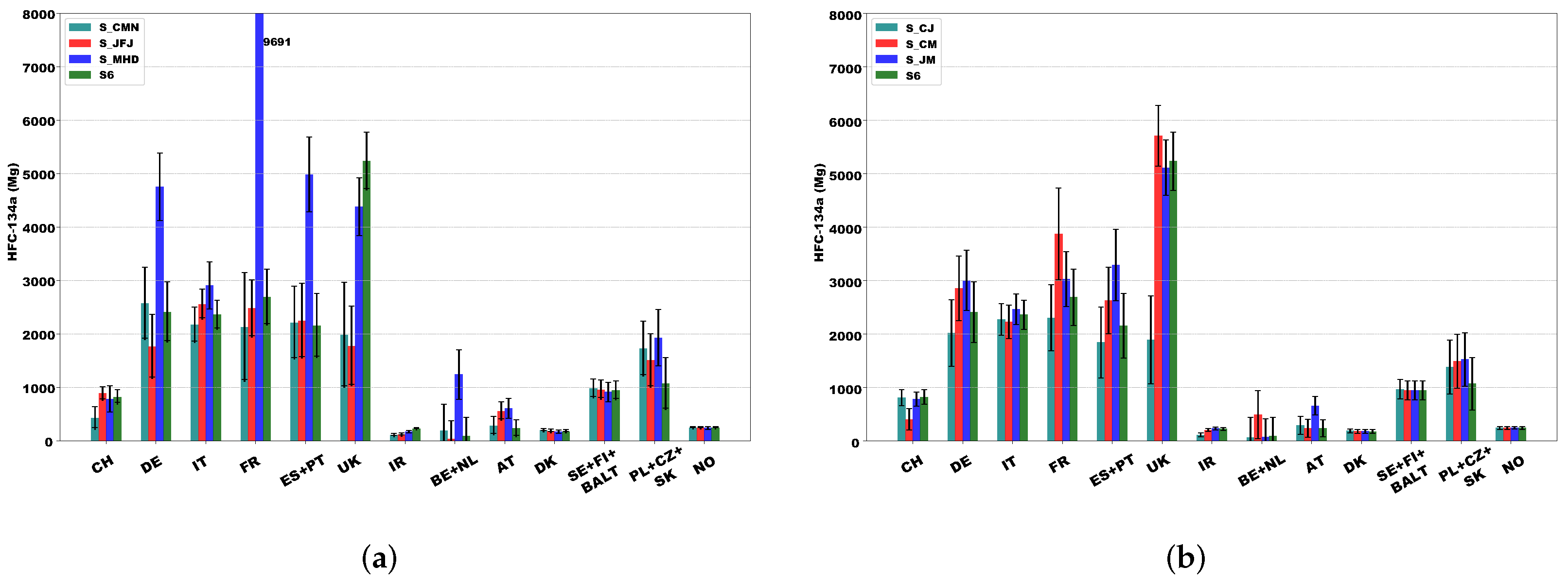
• Simulations S_CMN, S_JFJ, and S_MHD are inversions that exclusively use data from the CMN, JFJ, and MHD stations, respectively.
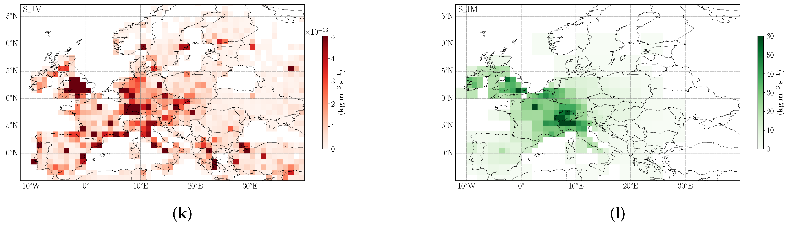
• Similarly, the simulations S_CJ, S_CM, and S_JM combine observations from the CMN and JFJ, CMN and MHD, and JFJ and MHD sites, respectively.

These simulations provide valuable insights into the sensitivity of inversions to the choice of receptor sites, including their locations and the number of receptors utilized in the analysis.

3. Results

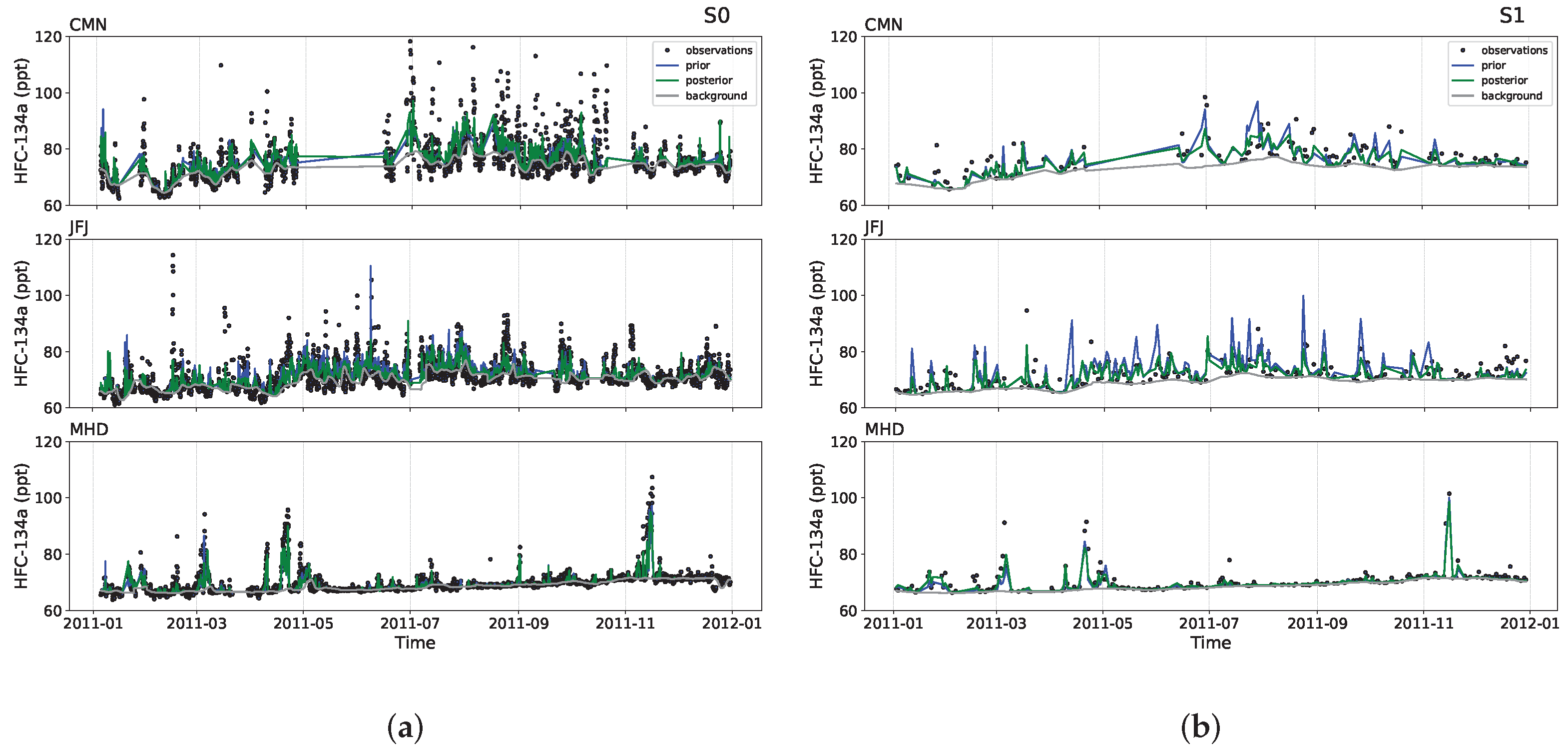
3.1. Simulated Time Series

Figure 3 illustrates the simulated prior and posterior time series compared to the observations for all measurement stations in S0 and S1 (definitions provided in Table 3). In both cases, the simulated prior mixing ratios align with the major peaks in the observation data. This suggests that the Lagrangian Particle Dispersion Model (FLEXPART) is proficient in capturing much of the observed variability in HFC-134a mixing ratios attributed to transport and meteorology. Furthermore, the posterior modelled mixing ratios, as shown in the figure, indicate that the inversion setup successfully narrows the gap between the simulated prior and observed mixing ratios. In simulation S5, the REBS method was employed to estimate the background mixing ratios. Figure 4 illustrates that the baseline determined by the REBS algorithm is generally higher than the baseline determined using the 2-PDF method. Notably, this difference is more pronounced for mountain stations compared to sea-level stations. The average background mixing ratio in the REBS method is higher by 2.6 ppt, 1.8 ppt, and 0.5 ppt for CMN, JFJ, and MHD, respectively, in comparison to the 2-PDF method. In simulations S6 and S7, background mixing ratios were optimized within the inversion system. As shown in Figure 4 the optimized background mixing ratios tend to fall between the values determined using the two methods. The optimized baseline in simulation S6, based on the REBS method, is lower than the REBS baseline, while for simulation S7, the optimized baseline, based on the 2-PDF method, is higher than the 2-PDF baseline. This suggests that the optimization of the baseline in inversion aims to improve the baseline and reduce the bias in the posterior estimate.

Figure 5 serves as a comprehensive representation of the quantitative model performance evaluation. In this figure, the Taylor plot is employed to visually depict the normalized standard deviation and correlation for both prior and posterior simulated mixing ratios in comparison to observations at each station. In Figure 5a, the relationship between prior and posterior simulated mixing ratios for each station and observations is presented for different simulations. It’s evident that the prior simulated mixing ratios (hollow markers) exhibit a wide spread with high standard deviation and low correlation. However, for posterior mixing ratios (filled markers), there is a noticeable reduction in standard deviation, along with an improved correlation, indicating significant model performance enhancement. Figure 5b depicts a histogram of the mismatch between modelled mixing ratios and observed values, both before and after the inversion for simulation S6. The standard deviation for the prior simulated mixing ratios is 3.3 ppt, while the posterior standard deviation is reduced to 2.7 ppt. This reduction in standard deviation indicates an improvement due to the model’s ability to better align with the observed data following the inversion.

Table 4. Comparison of R, RMSE, and NSD errors for different simulations.

Test	R						RMSE						NSD
	Prior			Posterior			Prior			Posterior			Prior			Posterior
	CMN	JFJ	MHD	CMN	JFJ	MHD	CMN	JFJ	MHD	CMN	JFJ	MHD	CMN	JFJ	MHD	CMN	JFJ	MHD
S0	0.57	0.54	0.84	0.62	0.58	0.86	7.11	4.34	2.17	6.81	3.99	2.03	0.56	0.82	0.71	0.61	0.71	0.73
S1	0.68	0.62	0.86	0.75	0.75	0.89	4.37	4.62	2.52	3.73	2.9	2.22	1.04	1.38	0.75	0.87	0.91	0.74
S2	0.71	0.67	0.88	0.76	0.76	0.89	3.87	3.39	2.19	3.73	2.83	2.27	0.86	1.02	0.76	0.82	0.86	0.68
S3	0.7	0.67	0.86	0.74	0.76	0.89	4.18	3.35	2.66	3.77	2.83	2.1	0.8	0.98	0.64	0.85	0.9	0.75
S4	0.57	0.49	0.7	0.61	0.58	0.86	7.22	4.3	2.8	6.85	3.99	1.97	0.46	0.62	0.54	0.61	0.71	0.75
S5	0.72	0.67	0.86	0.77	0.77	0.88	3.88	3.66	2.48	3.39	2.67	2.26	0.85	1	0.64	0.77	0.76	0.7
S6	0.72	0.67	0.86	0.77	0.77	0.88	3.88	3.66	2.48	3.42	2.64	2.23	0.85	1	0.64	0.76	0.78	0.74
S7	0.7	0.67	0.86	0.75	0.78	0.88	4.18	3.35	2.66	3.55	2.62	2.19	0.8	0.98	0.64	0.77	0.81	0.73

provides a summary of statistical error parameters, including R (Pearson’s correlation), RMSE (root mean squared error), and NSD (normalized standard deviation) for the conducted sensitivity tests. NSD is a measure of the model’s standard deviation normalized by the standard deviation of the observations. It’s noteworthy that simulation S6 and S7 demonstrate the most substantial improvement in these parameters when compared to the other tests, underlining the effectiveness of the implemented changes.

3.2. Emissions Fluxes

Figure 6 displays the gridded posterior emission fluxes at a model spatial resolution of 1° × 1° for sensitivity tests involving different prior datasets. These tests used EDGARv4.2, EDGARv6.0, EDGARv7.0, and a flat distributed a priori map for simulations S1, S2, S3, and S4, respectively. Despite the substantial differences in prior distributions, as shown in Figure 1, the inversion algorithm yields similar posterior distributions. Notably, even in simulation S4, which employs a flat prior distribution, the algorithm correctly identifies primary emission hotspots. These sensitivity tests underscore the ability of the inversion setup to converge to a consistent a posteriori solution, indicating a limited sensitivity to the prior information.

The results identify high-emitting regions with high confidence in Central Europe, Italy, and the UK for HFC-134a. The right panel of Figure 6 illustrates emission updates, representing the difference between the posterior and prior emission flux. Positive values observed over the UK and southern Europe in inversions S1 and S3 indicate that the EDGAR v4.2 and EDGAR v7.0 have lower flux compared to our results in these regions. In contrast, the high negative values over Western Europe in inversion S2 suggest that EDGAR v6.0 is higher compared to our posterior flux.

Figure 7 illustrates the posterior emission fluxes and the reduction in uncertainty for simulations conducted with various combinations of receptor sites. The right panel of the figure displays the difference between the posterior and prior uncertainties, normalized by the prior uncertainty. These results highlight how the posterior emission fluxes are influenced by the sensitivity of the observation data and the placement of the monitoring sites. Although there are substantial variations in the posterior emission fluxes across different regions, they consistently identify the same primary emission hotspots. The simulation S_CMN (Figure 7a) and S_JFJ, (Figure 7c) produce similar posterior emission flux because of the proximity of CMN and JFJ measurement sites with respect to MHD. The inclusion of observations from MHD in the inversion process unveils significant emission hotspots in Western Germany. It indicates that the observation stations CMN and JFJ complement each other to a large extent, with MHD providing a stronger overall constraint on our domain.

The uncertainty reduction maps reveal a notable decrease in the estimated uncertainties. Specifically, the regions in close proximity to the observation sites exhibit the most substantial reduction in uncertainty. This underscores the idea that augmenting the number of measurement stations leads to more accurate and improved emission estimates.

3.3. Country-Aggregated Emissions

The main application of atmospheric inversions is to quantify the GHG emissions at the country scale to verify their commitments towards different international treaties. We aggregate the posterior emission fluxes to get the country-wise totals: Figure 8a shows the total prior emission for each country from different a priori datasets; in Figure 8b the posterior total emissions for simulations S1, S2, S3, and S4 are shown. Notably, the prior national total emissions differ significantly for Germany, Italy, and Spain + Portugal when using different priors. However, despite these variations in the prior estimates, the posterior national total emissions tend to converge and show good agreement across different simulations. The inversion using a flat prior (S4), is expected to yield relatively lower prior national emissions for high-emitting countries and relatively higher prior emissions for low-emitting countries. Nevertheless, for the countries well constrained by the measurement network (CH, DE, IT, FR, ES + PT, UK, IR, and BE + NL) the inversion effectively corrects and refines these estimates, resulting in posterior national totals that fall within a similar range as other inversion result performed using EDGAR priors. This underscores that the estimates for these countries are better informed by the measurements than by the prior estimate.

Table 5. Emissions of HFC-134a for the different sensitivity experiments for major countries in Western Europe. UNFCCC refers to the 2011 emissions according to the country reports submitted to UNFCCC in 2013. The EDGAR estimates are calculated from an aggregation of the prior flux used in the inversions.

Simulation	DE (Mg·yr−1)	IT (Mg·yr−1)	FR (Mg·yr−1)	UK (Mg·yr−1)	ES + PT (Mg·yr−1)
S0	$4735\pm 475$	$3473\pm 197$	$4247\pm 294$	$2805\pm 389$	$2846\pm 403$
S1	$3045\pm 934$	$3396\pm 383$	$3514\pm 662$	$5204\pm 590$	$3061\pm 545$
S2	$3602\pm 546$	$4384\pm 449$	$3569\pm 532$	$4381\pm 595$	$2647\pm 911$
S3	$3624\pm 548$	$3463\pm 257$	$3888\pm 491$	$5295\pm 515$	$3523\pm 567$
S4	$3234\pm 156$	$3240\pm 123$	$4439\pm 162$	$2686\pm 107$	$3059\pm 274$
S5	$1861\pm 548$	$2199\pm 257$	$2346\pm 491$	$5319\pm 516$	$1636\pm 567$
S6	$2408\pm 568$	$2358\pm 275$	$2688\pm 528$	$5233\pm 546$	$2154\pm 603$
S7	$2982\pm 550$	$2900\pm 260$	$3144\pm 493$	$5032\pm 518$	$2568\pm 571$
S_CMN	$2570\pm 678$	$2170\pm 337$	$2130\pm 1018$	$1983\pm 983$	$2209\pm 686$
S_JFJ	$1766\pm 602$	$2556\pm 286$	$2477\pm 540$	$1773\pm 747$	$2247\pm 701$
S_MHD	$4758\pm 632$	$2909\pm 439$	$9691\pm 1021$	$4381\pm 538$	$4984\pm 700$
S_CJ	$2016\pm 621$	$2270\pm 298$	$2301\pm 617$	$1890\pm 822$	$1843\pm 664$
S_CM	$2852\pm 605$	$2225\pm 314$	$3869\pm 860$	$5707\pm 569$	$2625\pm 620$
S_JM	$3000\pm 564$	$2463\pm 284$	$3024\pm 513$	$5113\pm 520$	$3288\pm 666$
Median *	3140	3318	3542	5118	2747
Range *	1861–4735	2199–4384	2346–4439	2686–5319	1636–3523
UNFCCC 2011	4357	2523	5171	6178	3695
EDGARv4.2	6663	3723	5464	3832	2471
EDGARv6.0	4673	5135	6081	4315	5282
EDGARv7.0	4198	2188	4956	3334	3202
Median **	5026	3613	4237	3090	3545
Range **	2909–6823	2909–4958	3367–4970	2827–3227	2453–6437
EMPA **	$6745\pm 1465$	$3586\pm 387$	$3508\pm 465$	$2713\pm 432$	$2363\pm 485$
UKMO **	$3876\pm 1847$	$3450\pm 625$	$4966\pm 1206$	$3206\pm 855$	$3687\pm 745$

* Only S0, S1, S2, S3, S4, S5, and S6 are used to calculate the estimate; ** Estimates from the model configurations used in Brunner et al. for HFC-134a [16].

summarizes the emission estimates for well-constrained major countries namely, Germany (DE), Italy (IT), France (FR), United Kingdoms (UK), and Spain+Portugal (ES + PT) for all the sensitivity tests. The measurement network used in this study is not very sensitive to the emission in the eastern and north-eastern part of the domain(AT, NO, SE + FI + BALT, PO + CZ + SK), since the posterior emissions tend to be close to the prior emissions.

The inversions performed using different background mixing ratios (S3, S5, S6, and S7) show significant differences in the posterior national emission estimates. In Figure 9a it’s evident that simulation S5, which uses the REBS baseline, yields lower posterior emissions estimates for several countries when compared to S3, which uses the 2-PDF baseline. Specifically, there are reductions in emissions for Germany (49%), Italy (37%), France (40%), and Spain + Portugal (54%). This difference can be attributed to the higher background mixing ratios calculated by the REBS algorithm, as illustrated in Figure 4. In simulation S6, optimizing the REBS baseline leads to a slight increase in emission estimates. However, even in simulation S6, the emission estimates for Germany (34%), Italy (32%), France (31%), and Spain + Portugal (39%) remain lower than those in simulation S3. Finally, in S7, the optimization of the 2-PDF baseline is implemented, which is lower than the S3 estimates by 18% for Germany, 16% for Italy, 19% for France, and 27% for Spain + Portugal. The effect of different baseline algorithms is minimal on UK emissions (less than 5%). The emission estimates for S6 and S7 for these major countries agree well (within 4–24%) among themselves.

In Figure 9b, we compare the median emission estimates for major European countries from simulations S0 to S7 with those from the UNFCCC and the median estimates provided by Brunner et al. [16]. where 4 different inversion systems (EMPA, EMPA2, NILU, and UKMO) are used to estimate HFC-134a emissions. The error bars in this figure are the minimum and maximum estimates. The median estimates align closely for Italy, France, Spain + Portugal, Ireland, Poland + the Czech Republic + Slovenia, and Norway. However, their reported median UK HFC-134a emissions are 40% lower than those in our study and 50% lower than the UNFCCC-reported emissions. In contrast, our median UK emissions estimates are only 17% lower than the UNFCCC. There is a significant discrepancy in median HFC-134a emission estimates for Germany between the two studies, with Brunner et al. [16] estimating 60% higher than our results. Our national estimates for Switzerland, Italy, the UK, Ireland, Austria, Denmark, Sweden + Finland + Baltic countries (Estonia, Latvia, and Lithuania), and Norway are more closely aligned with the UNFCCC-reported estimates than those previously presented and, however fall within the range (minimum to maximum) of their results for nearly all countries.

The results from inversions that use different combinations of receptor sites are presented in Figure 10. Specifically, as illustrated in Figure 10a, when we exclusively rely on measurements from the MHD station, the posterior estimates for France show a substantial increase of 260%, while Spain + Portugal and Germany also exhibit increases of 131% and 98%, respectively, compared to the results in S6. Additionally, if we consider observations solely from either CMN or JFJ, the posterior estimates for the UK are approximately 65% higher than those in S6. Figure 10b shows a lower emission estimate for Switzerland for simulation S_CM compared with other simulations using two measurement stations highlighting the importance of the JFJ station. Similarly, it highlights the importance of the MHD station for estimating UK and Irish emissions.

4. Discussion

In this study on the evaluation of synthetic gas emissions using the FLEXINVERT+ inversion system, various sensitivity tests were conducted using as test compound the most abundant fluorocarbon, HFC-134a. Having as term of reference the results obtained by Brunner et al. [16], we chose the year 2011. These experiments assessed the system’s sensitivity to different factors, including the observation selection criteria, prior inventory, background mixing ratios, and the selection of observation stations used in the inversion process.

The LPDM model employed, FLEXPART, effectively simulated the prior mixing ratios. Pearson’s correlation coefficients for prior mixing ratios ranged from 0.57–0.72 at CMN, 0.49–0.67 at JFJ, and 0.7–0.88 at MHD. After the inversion, there were notable improvements, with correlation coefficients increasing to 0.61–0.77 at CMN, 0.58–0.78 at JFJ, and 0.86–0.89 at MHD. Simulations S6 and S7 exhibited the most significant improvements in posterior modelled mixing ratios. In S6 the Root Mean Square Error (RMSE) is reduced by 12%, 28%, and 10% at CMN, JFJ, and MHD, respectively. On the other hand, considering the Normalized Standard Deviation (NSD), which reflects the model’s ability to capture variability compared to measurements, the most significant improvement occurred in simulation S4, with increases of 33%, 15%, and 39% at CMN, JFJ, and MHD, respectively. This improvement was attributed to the use of a flat prior in S4, which was unable to catch most of the variability in prior simulated mixing ratios that were substantially optimised during the inversion. However, in simulation S6, the NSD deteriorated by 11% and 22% at CMN and JFJ, respectively. Conversely, at MHD, there is an improvement in NSD by 16%.

The inversion tests S0 and S4 used 10248 observations, while S1, S2, S3, S4, S5, S6, and S7 used 561 observations to constrain the emissions. The inversions without baseline optimization had 308 state variables and with baseline optimization 321(308 emission + 13 background) state variables. The posterior gridded emission fluxes based on different a priori information produced very similar posterior emissions. The emission updates for priors EDGARv 4.2 and EDGAR v7.0 both showed higher emissions compared to the priors over the UK, Ireland, Spain, and Italy. On the other hand, emissions for Germany and France were significantly reduced in the inversion with respect to the prior.

Inversions conducted using a single measurement station exhibited noticeable differences, primarily due to the limited ability of a single station to effectively constrain the entire spatial domain. For instance, in the simulation using only the MHD station, emissions were significantly increased over regions encompassing France, Germany, Spain, and Portugal. However, when two very distant observation stations were used in the inversions (as for example in the S_CM and S_JM simulations), the emissions were constrained well to some extent.

The inversion S0, carried out using all available observations was compared to the EMPA simulation as described in the study by Brunner et al. [16]. This comparison was made because the EMPA system used 3-hourly mean observations and yielded comparable results for the major emitting countries. The medians estimates reported in Table 5 and in Figure 9b was calculated using simulations S0 to S7 (simulations with all observation stations) and agrees well with the UKMO estimate for Germany and Italy, and with the EMPA estimate for France and Spain+Portugal. The variability in the national estimates from all simulations (S0–S7) is calculated as the $1\sigma$ standard deviation of an individual estimate, expressed as a percentage of the mean. The variability was in the range of 21–27%, the lowest for Italy and the highest for Germany.

The use of observations within a specific time window led to improvements in error statistics. However, this approach, which significantly reduced the number of observations available for inversion, necessitates more accurate prior information. Simulations involving different background algorithms revealed that the inversion setup is particularly sensitive to the background mixing ratios. Countries well-constrained by the observation network showed a significant reduction in emissions with a slightly higher baseline.

5. Conclusions

In this paper, we conducted a thorough examination of the synthetic greenhouse gas inversion system’s sensitivity to various model inputs through well-controlled experiments. We used FLEXINVERT+, a Bayesian inversion system, that utilized footprints generated by the FLEXPART LPDM model. The inversions were based on continuous HFC-134a observations from three locations within the AGAGE measurement network in the European domain. The sensitivity experiments conducted assessed the model’s sensitivity to observation selection criteria, a priori information, background mixing ratios, and the number of receptors used in the inversion process.

Concerning observation selection criteria, two distinct time windows were selected based on station location (mountain or coastal station), contrasting against the entire dataset. Four different prior emission maps were employed in experiments evaluating sensitivities to the a priori emissions. Two observation-based algorithms were applied to determine background mixing ratios, and in two additional experiments, the background mixing ratios were optimized within the inversion. Lastly, a series of experiments utilized observations from specific stations, to understand the significance of station location and its information contribution to the overall inversion process.

Through the implementation of 14 sensitivity experiments, designed to assess the impact of various inputs on inversion estimates, we garnered valuable insight. Notably, the introduction of a well-informed observation selection criteria for challenging mountain stations has demonstrated a substantial improvement in the bias within the inversion system. Our inversion setup exhibits less sensitivity to a priori emissions, with the posterior emission flux primarily driven by observational data. While different algorithms employed for estimating background mixing ratios produced similar time series, significant disparities were observed in posterior national emission estimates. This underscores the critical importance of accurately estimating background mixing ratios. The two optimized background mixing ratio time series fell between the two estimated background mixing ratio time series. Furthermore, tests conducted using individual receptors underscored their significance in constraining emissions across the study domain. These findings collectively contribute to a better understanding of the factors influencing inversion estimates and enhance the reliability of our greenhouse gas emission assessments.

The observation network and the limited time series used in this study restrain the coverage for effective inverse modelling estimates over the entire domain. However, it is able to constrain the broad spatial patterns and to identify discrepancies with reported national emissions of synthetic gases to UNFCCC, suggesting that a collaboration between these communities can provide much more to increase the accuracy of the inventories. This is a crucial aspect essential for gaining a more holistic understanding of shifts in regional emissions by incorporating both bottom-up and top-down approaches. It could also enhance the assessment of the implementation of environmental policies, particularly those addressing climate change, involving compounds such as the one under consideration. This need for a more precise evaluation of policy implementation has been reiterated in the latest release of the Emissions Gap Report 2023 by UNEP [52]. Future improvements are expected by applying our revised and optimized methodology to a wider observing network i.e., using the most recently introduced observing stations in the EU of Tacolneston(UK) and Taunus(DE)-, for longer time series and expanding the analysis to a wider range of long-lived compounds of interest, such as the HFCs used in the more recent air conditioning and heat-pump systems (HFC-152a, HFC-125, HFC-143a, HFC-32) for which a better understanding of emission is required.

References

1. IPCC. Climate Change 2021—The Physical Science Basis: Working Group I Contribution to the Sixth Assessment Report of the Intergovernmental Panel on Climate Change; Cambridge University Press: Cambridge, UK, 2021. [Google Scholar] [CrossRef]
2. IPCC. 2019 Refinement to the 2006 IPCC Guidelines for National Greenhouse Gas Inventories—IPCC; IPCC: Geneva, Switzerland, 2019. [Google Scholar]
3. Enting, I.G. Inverse Problems in Atmospheric Constituent Transport; Medium: Electronic Resource; Cambridge University Press: Cambridge, UK; New York, NY, USA, 2002. [Google Scholar]
4. Berchet, A.; Sollum, E.; Thompson, R.L.; Pison, I.; Thanwerdas, J.; Broquet, G.; Chevallier, F.; Aalto, T.; Berchet, A.; Bergamaschi, P.; et al. The Community Inversion Framework v1.0: A unified system for atmospheric inversion studies. Geosci. Model Dev. 2021, 14, 5331–5354. [Google Scholar] [CrossRef]
5. Katharopoulos, I.; Rust, D.; Vollmer, M.K.; Brunner, D.; Reimann, S.; O’Doherty, S.J.; Young, D.; Stanley, K.M.; Schuck, T.; Arduini, J.; et al. Impact of Transport Model Resolution and a Priori Assumptions on Inverse Modeling of Swiss F-gas Emissions. Atmos. Chem. Phys. 2023, 23, 14159–14186. [Google Scholar] [CrossRef]
6. Stell, A.C.; Bertolacci, M.; Zammit-Mangion, A.; Rigby, M.; Fraser, P.J.; Harth, C.M.; Krummel, P.B.; Lan, X.; Manizza, M.; Mühle, J.; et al. Modelling the growth of atmospheric nitrous oxide using a global hierarchical inversion. Atmos. Chem. Phys. 2022, 22, 12945–12960. [Google Scholar] [CrossRef]
7. Lian, J.; Lauvaux, T.; Utard, H.; Bréon, F.M.; Broquet, G.; Ramonet, M.; Laurent, O.; Albarus, I.; Chariot, M.; Kotthaus, S.; et al. Can we use atmospheric CO2 measurements to verify emission trends reported by cities? Lessons from a 6-year atmospheric inversion over Paris. Atmos. Chem. Phys. 2023, 23, 8823–8835. [Google Scholar] [CrossRef]
8. Petrescu, A.M.R.; Qiu, C.; McGrath, M.J.; Peylin, P.; Peters, G.P.; Ciais, P.; Thompson, R.L.; Tsuruta, A.; Brunner, D.; Kuhnert, M.; et al. The consolidated European synthesis of CH4 and N2O emissions for the European Union and United Kingdom: 1990–2019. Earth Syst. Sci. Data 2023, 15, 1197–1268. [Google Scholar] [CrossRef]
9. Miller, S.M.; Michalak, A.M.; Detmers, R.G.; Hasekamp, O.P.; Bruhwiler, L.M.P.; Schwietzke, S. China’s Coal Mine Methane Regulations Have Not Curbed Growing Emissions. Nat. Commun. 2019, 10, 303. [Google Scholar] [CrossRef]
10. Yao, B.; Fang, X.; Vollmer, M.K.; Reimann, S.; Chen, L.; Fang, S.; Prinn, R.G. China’s Hydrofluorocarbon Emissions for 2011–2017 Inferred from Atmospheric Measurements. Environ. Sci. Technol. Lett. 2019, 6, 479–486. [Google Scholar] [CrossRef]
11. Velders, G.J.M.; Andersen, S.O.; Daniel, J.S.; Fahey, D.W.; McFarland, M. The importance of the Montreal Protocol in protecting climate. Proc. Natl. Acad. Sci. USA 2007, 104, 4814–4819. [Google Scholar] [CrossRef]
12. Stohl, A.; Seibert, P.; Arduini, J.; Eckhardt, S.; Fraser, P.; Greally, B.R.; Lunder, C.; Maione, M.; Mühle, J.; O’Doherty, S.; et al. An analytical inversion method for determining regional and global emissions of greenhouse gases: Sensitivity studies and application to halocarbons. Atmos. Chem. Phys. 2009, 9, 1597–1620. [Google Scholar] [CrossRef]
13. Hu, L.; Montzka, S.A.; Miller, J.B.; Andrews, A.E.; Lehman, S.J.; Miller, B.R.; Thoning, K.; Sweeney, C.; Chen, H.; Godwin, D.S.; et al. U.S. emissions of HFC-134a derived for 2008–2012 from an extensive flask-air sampling network. J. Geophys. Res. Atmos. 2015, 120, 801–825. [Google Scholar] [CrossRef]
14. Lunt, M.F.; Rigby, M.; Ganesan, A.L.; Manning, A.J.; Prinn, R.G.; O’Doherty, S.; Mühle, J.; Harth, C.M.; Salameh, P.K.; Arnold, T.; et al. Reconciling reported and unreported HFC emissions with atmospheric observations. Proc. Natl. Acad. Sci. USA 2015, 112, 5927–5931. [Google Scholar] [CrossRef] [PubMed]
15. Simmonds, P.G.; Rigby, M.; Manning, A.J.; Lunt, M.F.; O’Doherty, S.; McCulloch, A.; Fraser, P.J.; Henne, S.; Vollmer, M.K.; Mühle, J.; et al. Global and regional emissions estimates of 1,1-difluoroethane (HFC-152a, CH3CHF2) from in situ and air archive observations. Atmos. Chem. Phys. 2016, 16, 365–382. [Google Scholar] [CrossRef]
16. Brunner, D.; Arnold, T.; Henne, S.; Manning, A.; Thompson, R.L.; Maione, M.; O’Doherty, S.; Reimann, S. Comparison of four inverse modelling systems applied to the estimation of HFC-125, HFC-134a, and SF6 emissions over Europe. Atmos. Chem. Phys. 2017, 17, 10651–10674. [Google Scholar] [CrossRef]
17. Graziosi, F.; Arduini, J.; Furlani, F.; Giostra, U.; Cristofanelli, P.; Fang, X.; Hermanssen, O.; Lunder, C.; Maenhout, G.; O’Doherty, S.; et al. European emissions of the powerful greenhouse gases hydrofluorocarbons inferred from atmospheric measurements and their comparison with annual national reports to UNFCCC. Atmos. Environ. 2017, 158, 85–97. [Google Scholar] [CrossRef]
18. Manning, A.J.; Redington, A.L.; Say, D.; O’Doherty, S.; Young, D.; Simmonds, P.G.; Vollmer, M.K.; Mühle, J.; Arduini, J.; Spain, G.; et al. Evidence of a recent decline in UK emissions of hydrofluorocarbons determined by the InTEM inverse model and atmospheric measurements. Atmos. Chem. Phys. 2021, 21, 12739–12755. [Google Scholar] [CrossRef]
19. Kim, J.; Thompson, R.; Park, H.; Bogle, S.; Mühle, J.; Park, M.K.; Kim, Y.; Harth, C.M.; Salameh, P.K.; Schmidt, R.; et al. Emissions of Tetrafluoromethane (CF4) and Hexafluoroethane (C2F6) From East Asia: 2008 to 2019. J. Geophys. Res. Atmos. 2021, 126, e2021JD034888. [Google Scholar] [CrossRef]
20. Redington, A.L.; Manning, A.J.; Henne, S.; Graziosi, F.; Western, L.M.; Arduini, J.; Ganesan, A.L.; Harth, C.M.; Maione, M.; Mühle, J.; et al. Western European emission estimates of CFC-11, CFC-12 and CCl4 derived from atmospheric measurements from 2008 to 2021. Atmos. Chem. Phys. 2023, 23, 7383–7398. [Google Scholar] [CrossRef]
21. Say, D.; Manning, A.J.; O’Doherty, S.; Rigby, M.; Young, D.; Grant, A. Re-Evaluation of the UK’s HFC-134a Emissions Inventory Based on Atmospheric Observations. Environ. Sci. Technol. 2016, 50, 11129–11136. [Google Scholar] [CrossRef]
22. Keller, C.A.; Hill, M.; Vollmer, M.K.; Henne, S.; Brunner, D.; Reimann, S.; O’Doherty, S.; Arduini, J.; Maione, M.; Ferenczi, Z.; et al. European Emissions of Halogenated Greenhouse Gases Inferred from Atmospheric Measurements. Environ. Sci. Technol. 2012, 46, 217–225. [Google Scholar] [CrossRef]
23. Prinn, R.G.; Weiss, R.F.; Arduini, J.; Arnold, T.; DeWitt, H.L.; Fraser, P.J.; Ganesan, A.L.; Gasore, J.; Harth, C.M.; Hermansen, O.; et al. History of chemically and radiatively important atmospheric gases from the Advanced Global Atmospheric Gases Experiment (AGAGE). Earth Syst. Sci. Data 2018, 10, 985–1018. [Google Scholar] [CrossRef]
24. EU. EUR-Lex-32014R0517-EN-EUR-Lex, 2014. Doc ID: 32014R0517 Doc Sector: 3 Doc Title: Regulation (EU) No 517/2014 of the European Parliament and of the Council of 16 April 2014 on Fluorinated Greenhouse Gases and Repealing Regulation (EC) No 842/2006 Text with EEA Relevance. Available online: https://eur-lex.europa.eu/legal-content/EN/TXT/?uri=celex%3A32014R0517 (accessed on 1 September 2023).
25. Thompson, R.L.; Stohl, A. FLEXINVERT: An atmospheric Bayesian inversion framework for determining surface fluxes of trace species using an optimized grid. Geosci. Model Dev. 2014, 7, 2223–2242. [Google Scholar] [CrossRef]
26. Evangeliou, N.; Thompson, R.L.; Eckhardt, S.; Stohl, A. Top-down estimates of black carbon emissions at high latitudes using an atmospheric transport model and a Bayesian inversion framework. Atmos. Chem. Phys. 2018, 18, 15307–15327. [Google Scholar] [CrossRef]
27. Jia, M.; Evangeliou, N.; Eckhardt, S.; Huang, X.; Gao, J.; Ding, A.; Stohl, A. Black Carbon Emission Reduction Due to COVID-19 Lockdown in China. Geophys. Res. Lett. 2021, 48, e2021GL093243. [Google Scholar] [CrossRef] [PubMed]
28. Prinn, R.G.; Weiss, R.F.; Fraser, P.J.; Simmonds, P.G.; Cunnold, D.M.; Alyea, F.N.; O’Doherty, S.; Salameh, P.; Miller, B.R.; Huang, J.; et al. A history of chemically and radiatively important gases in air deduced from ALE/GAGE/AGAGE. J. Geophys. Res. Atmos. 2000, 105, 17751–17792. [Google Scholar] [CrossRef]
29. Janssens-Maenhout, G.; Crippa, M.; Guizzardi, D.; Muntean, M.; Schaaf, E. Emissions Database for Global Atmospheric Research; Version Version 4.2 (Time-Series); European Commission, Joint Research Centre (JRC): Brussels, Belgium, 2011. [Google Scholar]
30. Ferrario, F.M.; Crippa, M.; Guizzardi, D.; Muntean, M.; Schaaf, E.; Vullo, E.L.; Solazzo, E.; Olivier, J.; Vignati, E. EDGAR v6.0 Greenhouse Gas Emissions; European Commission, Joint Research Centre (JRC): Brussels, Belgium, 2021. [Google Scholar]
31. Commission, E.; Centre, J.R.; Olivier, J.G.J.; Guizzardi, D.; Schaaf, E.; Solazzo, E.; Crippa, M.; Vignati, E.; Banja, M.; Muntean, M.; et al. GHG Emissions of All World: 2021 Report; Publications Office of the European Union: Luxembourg, 2021. [Google Scholar]
32. Stohl, A.; Forster, C.; Frank, A.; Seibert, P.; Wotawa, G. Technical note: The Lagrangian particle dispersion model FLEXPART version 6.2. Atmos. Chem. Phys. 2005, 5, 2461–2474. [Google Scholar] [CrossRef]
33. Seibert, P.; Frank, A. Source-receptor matrix calculation with a Lagrangian particle dispersion model in backward mode. Atmos. Chem. Phys. 2004, 4, 51–63. [Google Scholar] [CrossRef]
34. Stohl, A.; Hittenberger, M.; Wotawa, G. Validation of the lagrangian particle dispersion model FLEXPART against large-scale tracer experiment data. Atmos. Environ. 1998, 32, 4245–4264. [Google Scholar] [CrossRef]
35. Seibert, P. Iverse Modelling with a Lagrangian Particle Disperion Model: Application to Point Releases Over Limited Time Intervals. In Air Pollution Modeling and Its Application XIV; Gryning, S.E., Schiermeier, F.A., Eds.; Springer: Boston, MA, USA, 2001; pp. 381–389. [Google Scholar] [CrossRef]
36. Cesari, R.; Paradisi, P.; Allegrini, P. Source identification by a statistical analysis of backward trajectories based on peak pollution events. Int. J. Environ. Pollut. 2014, 55, 94–103. [Google Scholar] [CrossRef]
37. Hersbach, H.; Bell, B.; Berrisford, P.; Hirahara, S.; Horányi, A.; Muñoz-Sabater, J.; Nicolas, J.; Peubey, C.; Radu, R.; Schepers, D.; et al. The ERA5 global reanalysis. Q. J. R. Meteorol. Soc. 2020, 146, 1999–2049. [Google Scholar] [CrossRef]
38. Copernicus Climate Change Service. Complete ERA5 Global Atmospheric Reanalyis. 2023. Available online: https://cds.climate.copernicus.eu/cdsapp#!/dataset/10.24381/cds.143582cf?tab=overview (accessed on 1 September 2023).
39. Tipka, A.; Haimberger, L.; Seibert, P. Flex_extract v7.1.2—A software package to retrieve and prepare ECMWF data for use in FLEXPART. Geosci. Model Dev. 2020, 13, 5277–5310. [Google Scholar] [CrossRef]
40. Giostra, U.; Furlani, F.; Arduini, J.; Cava, D.; Manning, A.J.; O’Doherty, S.J.; Reimann, S.; Maione, M. The determination of a “regional” atmospheric background mixing ratio for anthropogenic greenhouse gases: A comparison of two independent methods. Atmos. Environ. 2011, 45, 7396–7405. [Google Scholar] [CrossRef]
41. Ruckstuhl, A.F.; Henne, S.; Reimann, S.; Steinbacher, M.; Vollmer, M.K.; O’Doherty, S.; Buchmann, B.; Hueglin, C. Robust extraction of baseline signal of atmospheric trace species using local regression. Atmos. Meas. Tech. 2012, 5, 2613–2624. [Google Scholar] [CrossRef]
42. Pérez, I.A.; Sánchez, M.L.; García, M.A. CO2 dilution in the lower atmosphere from temperature and wind speed profiles. Theor. Appl. Clim. 2012, 107, 247–253. [Google Scholar] [CrossRef]
43. Griffiths, A.D.; Conen, F.; Weingartner, E.; Zimmermann, L.; Chambers, S.D.; Williams, A.G.; Steinbacher, M. Surface-to-mountaintop transport characterised by radon observations at the Jungfraujoch. Atmos. Chem. Phys. 2014, 14, 12763–12779. [Google Scholar] [CrossRef]
44. Fang, S.X.; Tans, P.P.; Steinbacher, M.; Zhou, L.X.; Luan, T. Comparison of the regional CO2 mole fraction filtering approaches at a WMO/GAW regional station in China. Atmos. Meas. Tech. 2015, 8, 5301–5313. [Google Scholar] [CrossRef]
45. Maione, M.; Graziosi, F.; Arduini, J.; Furlani, F.; Giostra, U.; Blake, D.R.; Bonasoni, P.; Fang, X.; Montzka, S.A.; O’Doherty, S.J.; et al. Estimates of European emissions of methyl chloroform using a Bayesian inversion method. Atmos. Chem. Phys. 2014, 14, 9755–9770. [Google Scholar] [CrossRef]
46. Graziosi, F.; Arduini, J.; Bonasoni, P.; Furlani, F.; Giostra, U.; Manning, A.J.; McCulloch, A.; O’Doherty, S.; Simmonds, P.G.; Reimann, S.; et al. Emissions of carbon tetrachloride from Europe. Atmos. Chem. Phys. 2016, 16, 12849–12859. [Google Scholar] [CrossRef]
47. Henne, S.; Brunner, D.; Oney, B.; Leuenberger, M.; Eugster, W.; Bamberger, I.; Meinhardt, F.; Steinbacher, M.; Emmenegger, L. Validation of the Swiss methane emission inventory by atmospheric observations and inverse modelling. Atmos. Chem. Phys. 2016, 16, 3683–3710. [Google Scholar] [CrossRef]
48. Vollmer, M.K.; Mühle, J.; Trudinger, C.M.; Rigby, M.; Montzka, S.A.; Harth, C.M.; Miller, B.R.; Henne, S.; Krummel, P.B.; Hall, B.D.; et al. Atmospheric histories and global emissions of halons H-1211 (CBrClF2), H-1301 (CBrF3), and H-2402 (CBrF2CBrF2). J. Geophys. Res. Atmos. 2016, 121, 3663–3686. [Google Scholar] [CrossRef]
49. Schoenenberger, F.; Henne, S.; Hill, M.; Vollmer, M.K.; Kouvarakis, G.; Mihalopoulos, N.; O’Doherty, S.; Maione, M.; Emmenegger, L.; Peter, T.; et al. Abundance and sources of atmospheric halocarbons in the Eastern Mediterranean. Atmos. Chem. Phys. 2018, 18, 4069–4092. [Google Scholar] [CrossRef]
50. Vojta, M.; Plach, A.; Thompson, R.L.; Stohl, A. A comprehensive evaluation of the use of Lagrangian particle dispersion models for inverse modeling of greenhouse gas emissions. Geosci. Model Dev. 2022, 15, 8295–8323. [Google Scholar] [CrossRef]
51. Bergamaschi, P.; Corazza, M.; Karstens, U.; Athanassiadou, M.; Thompson, R.L.; Pison, I.; Manning, A.J.; Bousquet, P.; Segers, A.; Vermeulen, A.T.; et al. Top-down estimates of European CH4 and N2O emissions based on four different inverse models. Atmos. Chem. Phys. 2015, 15, 715–736. [Google Scholar] [CrossRef]
52. UN Environment Programme. Emissions Gap Report 2023: Broken Record—Temperatures Hit New Highs, yet World Fails to Cut Emissions (Again). Available online: https://wedocs.unep.org/20.500.11822/43922 (accessed on 1 September 2023).
Figure 1. The different a priori emission flux maps used in the inversion sensitivity experiments. Namely EDGAR v4.2 (a), EDGAR v6.0 (b), EDGAR v7.0 (c) and a flat prior (d).
Atmosphere 15 00051 g001
Figure 2. Total emission sensitivity in units of log(s m−3 kg−1) calculated using FLEXPART (a); the red triangles indicate the observation sites used in this study. Variable resolution grid used in the inversion based on the sensitivity information (b).
Atmosphere 15 00051 g002
Figure 3. Comparison of prior (blue line) and posterior (green line) simulated mixing ratios with observations (black dots) for simulations S0 (a) and S1 (b). The grey line represents the background mixing ratios used in the inversions.
Atmosphere 15 00051 g003
Figure 4. Time series of different background mixing ratios used in the inversions. The upper panel, middle panel, and lower panel show background mixing ratios at CMN, JFJ, and MHD stations, respectively. The dashed lines represent the optimized background mixing ratio time series.
Atmosphere 15 00051 g004
Figure 5. Taylor plot pertaining to all the simulations. The marker’s shape indicates the specific observation site, while different colours are used to distinguish between various simulations. The hollow markers correspond to prior mixing ratios and the filled markers correspond to the posterior mixing ratios. In the Taylor diagram, the linear distance from the reference point (the black hollow circle on the X-axis) is directly proportional to the centred root mean square error (RMSE). Simultaneously, the angle of rotation concerning the vertical axis corresponds to the Pearson correlation coefficient R (a). Histogram plot of the mismatch between the modelled mixing ratios and observations for both prior (in blue) and posterior (in green) modelled mixing ratios for simulation S6 (b).
Atmosphere 15 00051 g005
Figure 6. A posteriori emission fluxes of HFC-134a (left panels) and the difference between posterior and prior flux (right panels) for different sensitivity tests: S1 (a,b), S2 (c,d), S3 (e,f), and S4 (g,h) performed using EDGARv4.2, EDGARv6.0, EDGARv7.0 and a flat prior, respectively.
Atmosphere 15 00051 g006
Figure 7. Posterior flux, (left panels) and uncertainty reduction (1-epost/eprior) in percentage, (right panels) for simulations done using different combinations of receptors: CMN alone (a,b), JFJ alone (c,d), MHD alone (e,f), CMN with JFJ (g,h), CMN with MHD (i,j), JFJ with MHD (k,l).
Atmosphere 15 00051 g007aAtmosphere 15 00051 g007b
Figure 8. Prior total emissions for different countries for different a priori maps used in this study (a). The aggregated posterior total emissions for the different simulations (b). Country codes are as follows, CH = Switzerland, DE = Germany, IT = Italy, FR = France, ES = Spain, PT = Portugal, UK = United Kingdom, IR = Ireland, BE = Belgium, NL = Netherlands, AT = Austria, DK = Denmark, SE = Sweden, FI = Finland, BALT = Baltic countries (Estonia, Latvia, and Lithuania), PO = Poland, CZ = Czech Republic, SK = Slovakia, and NO = Norway.
Atmosphere 15 00051 g008
Figure 9. Posterior national emission estimates for inversions performed using different background mixing ratios (a). Median calculated using simulations S0 to S7 (b) compared with the estimates reported to UNFCCC and the median estimate for different modelling setups used in Brunner et al. [16]. Error bars represent the range of estimates.
Atmosphere 15 00051 g009
Figure 10. Comparison of posterior total emissions at national level for inversions done with different combinations of receptor sites: single (a) and paired (b) receptors used, against S6-all receptors.
Atmosphere 15 00051 g010