Spatial Distribution Characteristics and Analysis of PM_2.5 in South Korea: A Geographically Weighted Regression Analysis

Abstract

PM_2.5, a critical air pollutant, requires health-conscious management, with concentrations varying across regions due to diverse sources. This study, conducted in South Korea in 2021, employed the geographically weighted regression model to analyze the spatiotemporal correlations of PM_2.5 with O₃ and the normalized difference vegetation index (NDVI). Regional differences in the correlation between PM_2.5 and O₃ were observed, influenced by common precursors (SOx, NOx, and volatile organic compounds (VOCs)), seasonal temperature variations, and solar radiation differences. Notably, PM_2.5 and O₃ exhibited a heightened regression coefficient in summer, emphasizing the need for specific management targeting VOCs and NO₂. The interplay between PM_2.5 and NDVI revealed a negative overall impact but a positive effect in the central region of Korea, suggesting vegetation’s role in the PM_2.5 concentration increase due to atmospheric stagnation caused by mountain ranges. These findings enhance our understanding of PM_2.5 distribution mechanisms, highlighting the need for tailored policies in each region for effective concentration reductions.

1. Introduction

Air pollution, exacerbated by industrialization, has become a pressing environmental concern [1]. Of all air pollutants, PM_2.5, particulate matter (PM) with an aerodynamic equivalent diameter of 2.5 µm or less, is particularly significant. Due to its large surface area, PM_2.5 efficiently adsorbs toxic materials, accumulating them deep within the body [2]. Recognized as a Group 1 carcinogen by the International Agency for Research on Cancer under the World Health Organization [3], PM_2.5 poses a substantial health risk.

PM_2.5 stems from both artificial and natural sources [4]. Artificial sources include vehicle emissions, fugitive dust from construction sites, incineration facility smoke, and fossil fuel soot [5]. Natural sources encompass volcanic ash, pollen, dust from forest fires, and yellow dust [6]. Primary sources involve solid particles directly emitted, while secondary sources generate PM_2.5 through chemical reactions from gaseous substances in the atmosphere [7,8,9].

PM_2.5 is influenced by atmospheric precursors, industrial processes, forest fires, waste incineration, and natural resource combustion [5,6,8]. In addition, PM_2.5 has high transportability, so it is evenly distributed in a large area, but it shows different distribution patterns for each region depending on the source of the emission and the weather [10].

Given the regional variability in PM_2.5 concentration, various geographic information system methods have emerged, with the geographically weighted regression (GWR) model proving effective for spatial PM_2.5 analysis [11,12]. In a GWR analysis studying PM_2.5, O₃, and weather factors [13], PM_2.5 and O₃ showed different correlations depending on the season in the south and north, and the O₃ concentration was highest when the PM_2.5 concentration was approximately 50 μg/m³. In a study that conducted GWR analysis for PM_2.5 and architectural environment [14], GWR was performed for surrounding architectural environments, such as roads and green areas, revealing a positive correlation between PM_2.5 and areas with many artificial structures. The GWR model proves useful in identifying spatially variable factors, providing a method to address issues interpreted with a singular result, neglecting regional diversity [11]. GWR accounts for spatial diversity, offering accurate insights into regional changes and factors [12]. In GWR model studies for PM_2.5, O₃, and normalized difference vegetation index (NDVI), these variables, especially O₃ and NDVI, are commonly used and deemed valuable. This study focused on these two independent variables due to their intricate interactions with PM_2.5.

Therefore, this study sought to analyze the spatial distribution of PM_2.5 using the GWR model, with the goal of formulating region-specific countermeasures against PM_2.5. Building on this, a comparative analysis of PM_2.5 with O₃ and NDVI was conducted to explore the characteristics of PM_2.5 concentration in 2021 and discern spatial heterogeneity.

2. Materials and Methods

2.1. Study Area

This study encompassed South Korea, situated between longitudes 124° and 131° E and latitudes 33° and 38° N (Figure 1). South Korea experiences a range of climatic influences, with cold and dry continental pressure prevailing in winter and hot and humid oceanic pressure in summer. The annual average temperature is 13.2 °C, with minimum and maximum annual averages of 8.9 °C and 17.5 °C, respectively. Annual precipitation totals 1237.4 mm, with a concentration of 638.7 mm during the summer rainy season. Positioned in the mid-latitude temperate zone, the region exhibits distinct seasonality [15].

Characterized by numerous mountain ranges, South Korea features complex coastlines along its eastern, southern, and western sides. The altitude varies, with the east exhibiting higher elevations exceeding 1000 m, while the west remains predominantly below 200 m (Figure 1). Over the years, South Korea has witnessed an increase in air pollutants, attributed to rapid development and industrialization since the 1960s. The Seoul metropolitan area and some industrial cities, experiencing rapid economic growth, display significant differences in population density, leading to varied causes for air pollutant distribution across different regions.

2.2. Dataset Materials

2.2.1. Air Pollution Data

This study utilized data spanning from 1 January to 31 December 2021. O₃ and PM_2.5 were designated as the focal air pollutants, and concentration data obtained from 619 air pollution monitoring stations across 16 administrative districts in Korea were employed. For O₃, 8 h average data were utilized in adherence to the atmospheric environmental standards of Korea, the United States, and Europe. The air pollutant data used in this study for Korea are accessible as open data on Air Korea’s website (https://www.airkorea.or.kr/web/, accessed on 1 March 2023, operating agency: Korea Environment Corporation, Incheon, Republic of Korea). The PM_2.5 and O₃ data used in this study were measured by the β-Ray Absorption Method and the U.V Photometric Method, respectively.

2.2.2. NDVI

NDVI is a method for assessing the vitality of vegetation by calculating the difference between the red light absorbed by plants (400 to 700 nm) and the near-infrared ray reflected by them (700 to 1100 nm). The NDVI value ranges from −1 to 1, with a value close to 1, indicating healthy and dense vegetation. The NDVI data in 2021 were derived from MOD13Q1 (MODIS/Terra Vegetation Indices 16-Day L3 Global 250-m SIN Grid v006) provided by NASA’s Terra satellite, launched in 1999. NDVI is accessible as open data on EARTHDATA’s website (https://www.earthdata.nasa.gov/, accessed on 2 March 2023, operating agency: NASA, Washington, DC, USA). NDVI is calculated using Equation (1), where NIR represents the near-infrared ray, and Red represents the red light.

$$\mathrm{N}\mathrm{D}\mathrm{V}\mathrm{I}=\frac{(\mathrm{NIR}-\mathrm{R}\mathrm{e}\mathrm{d})}{(\mathrm{NIR}+\mathrm{R}\mathrm{e}\mathrm{d})}$$

(1)

2.2.3. Meteorological Data

The meteorological data incorporated in this study encompass temperature, relative humidity, precipitation, pressure, and wind speed. Daily average data from 95 Automated Synoptic Observing System points in 2021 were processed into monthly averages, serving as independent variables for PM_2.5 prediction. These meteorological data are accessible as open data on the Korea Meteorological Administration (KMA) portal (https://data.kma.go.kr/, accessed on 2 March 2023, operating agency: KMA, Daejeon, Republic of Korea).

2.3. Methods

All data were transformed into monthly average data and spatially interpolated using kriging with each measurement point and coordinate data. The analysis was conducted with a 0.05° horizontal and vertical grid (approximately 5.5 × 7.9 km), centered around Seoul for inland areas of Korea (excluding islands and coastlines). The GWR model was constructed using the processed variables. Regression coefficients for the independent variables of O₃ and NDVI were examined through the GWR model to assess their spatiotemporal correlations with PM_2.5. To ensure uniformity, all variables, having different units, were standardized for use in the GWR model.

2.3.1. Empirical Bayesian Kriging

Kriging, a spatial interpolation technique in geostatistics, predicts values at unmeasured locations based on measured data by assessing spatial dependence through a semivariogram and calculating optimal weights [16]. In this study, the Empirical Bayesian kriging (EBK) method was chosen among various kriging techniques. EBK employs the empirical Bayesian method to analyze additional distributed structures and mitigate the impact of abnormal variables and obtain improved results, even in limited cases [17]. Because of these advantages, EBK was used. All EBK model results utilized in this study were generated using ArcToolbox version ArcGIS Pro 2.8.

2.3.2. Pearson’s Correlation Coefficient Method

Pearson’s correlation analysis serves to identify the linear correlation between two variables, measuring the strength and direction of this relationship. A value close to 1 indicates a strong positive correlation, while a value near −1 suggests a strong negative correlation. A value near 0 signifies no correlation. In Equation (2), cov represents the covariance between the two variables X and Y, and ${\mathsf{\sigma }}_{\mathrm{X} }$ and ${\mathsf{\sigma }}_{\mathrm{Y}}$ denote the standard deviations for each variable. ${\mathrm{P}}_{\mathrm{X},\mathrm{Y}}$ is the Pearson correlation coefficient value. The results of Pearson’s correlation analysis in this study were obtained using IBM SPSS Statistics version 26.

$${\mathrm{P}}_{\mathrm{X},\mathrm{Y}}=\frac{\mathrm{c}\mathrm{o}\mathrm{v}(\mathrm{X},\mathrm{Y})}{{\mathsf{\sigma }}_{\mathrm{X}} {\mathsf{\sigma }}_{\mathrm{Y}}}$$

(2)

2.3.3. Variance Inflation Factor

The variance inflation factor (VIF) is employed to assess multicollinearity among independent variables. A rise in the VIF value indicates the presence of serious multicollinearity. A VIF value exceeding 1 suggests the existence of multicollinearity, while a VIF higher than 10 is indicative of a significant risk of analytical errors due to severe multicollinearity [18]. In Equation (3), VIF_i represents the VIF value of the i-th independent variable, and ${{\mathrm{R}}_{\mathrm{i}}}^2$ denotes the R² value obtained from the regression analysis results for the i-th variable with other independent variables. The VIF results utilized in this study were computed using IBM SPSS Statistics version 26.

$${\mathrm{V}\mathrm{I}\mathrm{F}}_{\mathrm{i}} = 1 / ( 1-{{\mathrm{R}}_{\mathrm{i}}}^2)$$

(3)

2.3.4. Global Moran’s Index

Global Moran’s index (Moran’s I) is a method for analyzing spatial autocorrelation, assessing the spatial cohesion of data on a scale from −1 to 1 [19]. When Moran’s I approaches 1, neighboring regions exhibit similar values, while values close to −1 indicate opposing values in neighboring regions. Moran’s I nearing 0 signifies no spatial autocorrelation. In Equation (4), $\mathrm{I}$ is the Global Moran’s index value. ${\mathrm{x}}_{\mathrm{i}}$ and ${\mathrm{x}}_{\mathrm{j}}$ represent measurements corresponding to i and j, respectively. ${\mathrm{S}}^2$ is the sample variance, $W_{ij}$ is the spatial weight matrix, and $\overline{\mathrm{x}}$ is the average of all measurements. $\mathrm{n}$ is the number of observation points. The Moran’s I results utilized in this study were computed using ArcToolbox version ArcGIS Pro 2.8.

$$\mathrm{I} = \frac{\sum _{\mathrm{i}=1}^{\mathrm{n}} \sum _{\mathrm{j}=1}^{\mathrm{n}} {\mathrm{W}}_{\mathrm{i}\mathrm{j}} ({\mathrm{x}}_{\mathrm{i}} - \overline{\mathrm{x}})( {\mathrm{x}}_{\mathrm{j}} - \overline{\mathrm{x}})}{{\mathrm{S}}^2\sum _{\mathrm{i}=1}^{\mathrm{n}} \sum _{\mathrm{j}=1}^{\mathrm{n}} {\mathrm{W}}_{\mathrm{i}\mathrm{j}} }$$

(4)

2.3.5. GWR Model

GWR is a regression analysis model that assigns weights based on geographic locations. Unlike fixing one regression coefficient for all measurements, GWR utilizes different regression coefficients by region. This model estimates optimal regression coefficients in each region, considering regional characteristics. In this study, the minimum corrected Akaike’s information criterion value was employed to derive the optimal GWR model. In Equation (5), ${\mathrm{y}}_{\mathrm{i}}$ represents the dependent variable. ${\mathrm{x}}_{\mathrm{i}\mathrm{k}}$ is the k-th independent variable, ${\mathrm{u}}_{\mathrm{i}}$ and ${\mathrm{a}}_{\mathrm{i}}$ are the coordinates of the is the measurement, ${\mathsf{\beta }}_{\mathrm{k}}$ is the regression coefficient of the independent variable, and ${\mathsf{\epsilon }}_{\mathrm{i}}$ is the error term. The GWR model results used in this study were computed using ArcToolbox version ArcGIS Pro 2.8.

$${\mathrm{y}}_{\mathrm{i}} = {\mathsf{\beta }}_0 ({\mathrm{u}}_{\mathrm{i}} , {\mathsf{\alpha }}_{\mathrm{i}}) + {\sum }_{\mathrm{i}=1}^{\mathrm{p}}{\mathsf{\beta }}_{\mathrm{k}} ({\mathrm{u}}_{\mathrm{i}} , {\mathsf{\alpha }}_{\mathrm{i}}) {\mathrm{x}}_{\mathrm{i}\mathrm{k}} + {\mathsf{\epsilon }}_{\mathrm{i}}$$

(5)

3. Results and Discussion

3.1. Analysis of Independent Variable Data

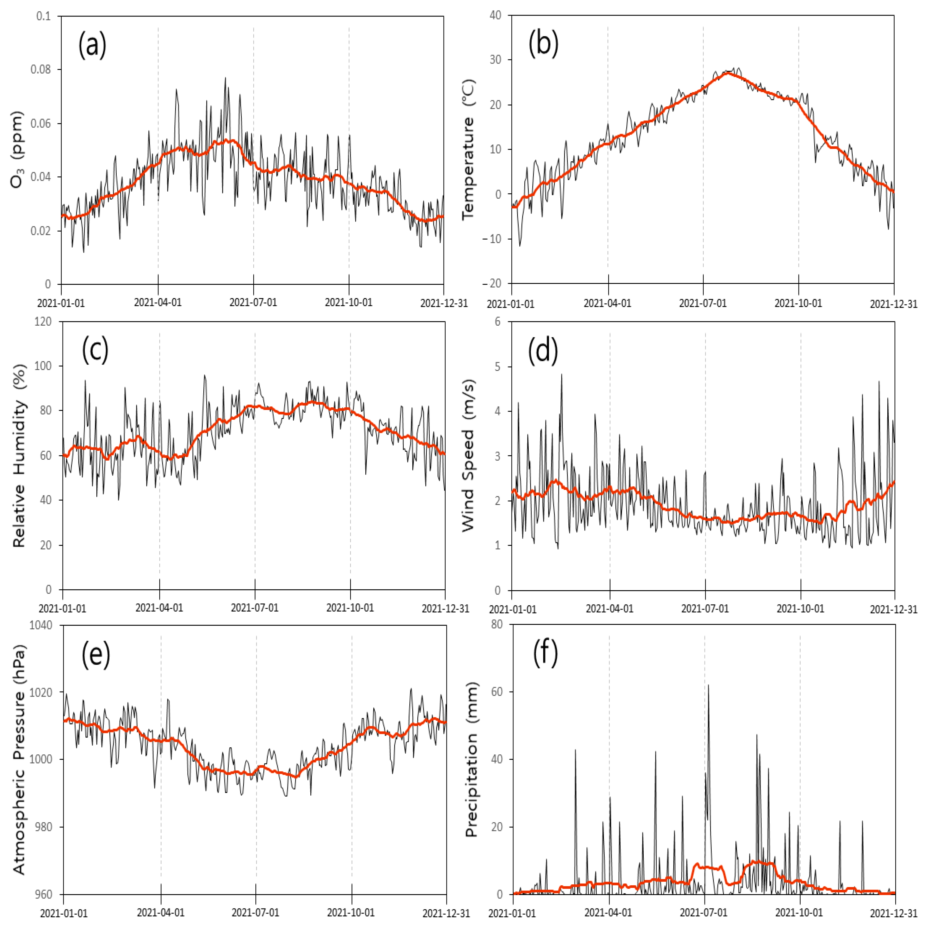
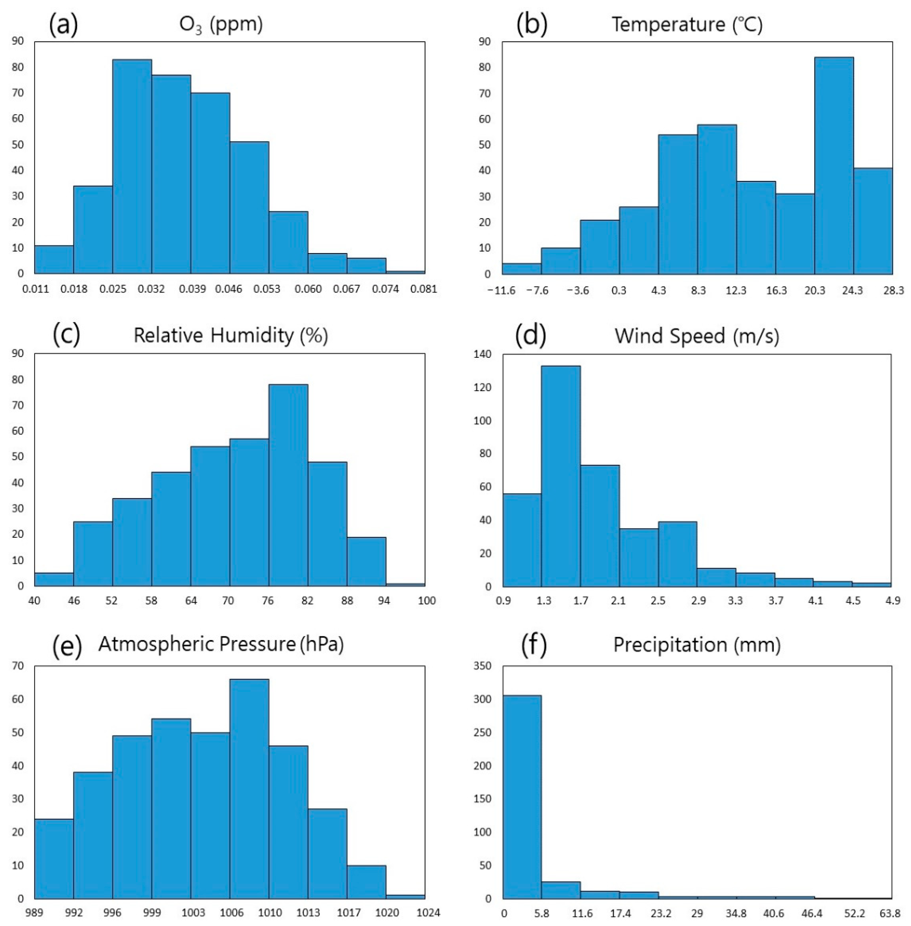
Figure 2 illustrates the daily and monthly averages of air pollutants and meteorological data used in this study for 2021, aggregated from all measurement stations. For precipitation, the daily sum was considered instead of the daily average. Figure 3 is a histogram that shows how the entire data are distributed. NDVI provided statistical results based on monthly data, indicating a peak in August with an average of approximately 0.7910 and the lowest point in January, with an average of 0.3768. O₃, temperature, humidity, and precipitation showed an increasing trend in July and August and a decreasing trend in January and December. In contrast, wind speed and atmospheric pressure increased in January and December and decreased in July and August. This finding aligns with previously reported meteorological patterns and air pollutant trends in South Korea [15,20]. Given the distinct four seasons in South Korea, the NDVI reached its peak value in August, corresponding to the northern hemisphere’s summer. Additionally, elevated temperatures, humidity, and precipitation were observed in July and August, coinciding with the warm summer season and the rainy season in South Korea.

The daily average concentration of O₃ reached its highest value (approximately 0.077 ppm) on 6 June and its lowest (0.011 ppm) on 22 January, gradually increasing from January and decreasing from June (Figure 2a). The monthly average concentration of O₃ peaked (approximately 0.053 ppm) on 6 June and hit its lowest point (0.025 ppm) in December (Figure 2a). O₃ concentration varied by month, being higher in relatively warm southern regions and lower in mountainous areas with abundant forests. The annual average temperature was 13 °C, with the daily average temperature reaching its highest (28 °C) on 5 August and lowest (−11 °C) on 8 January (Figure 2b). The temperature gradually increased from 1 January and then decreased from August (Figure 2b). The annual average relative humidity was approximately 71%, with the lowest humidity (around 40%) on 23 February and the highest (96%) on 16 May (Figure 2c). It was humid across the country from July to October and dry in January and December (Figure 2c). The daily average wind speed reached its lowest (0.9 m/s) on 14 February and its highest (4.8 m/s) on 17 February. Daily wind speed fluctuations were significant, with the maximum and minimum wind speeds occurring within three days and the annual average value being 1.9 m/s (Figure 2d). Daily wind speed changes decreased in July and August and increased in January and December (Figure 2d). The annual average atmospheric pressure was 1004 hPa, with the lowest atmospheric pressure (approximately 989 hPa) on 31 July and the highest (1021 hPa) on 28 November (Figure 2e). Atmospheric pressure decreased from January to July and increased from July to December (Figure 2e). Precipitation across the country in 2021 was approximately 1244 mm, with the highest precipitation (around 62 mm) observed on 6 July (Figure 2f). The monthly average precipitation was highest (approximately 9.2 mm) in August (Figure 2f). In the climate reports spanning from 1912 to 2017, the average temperature in Korea was 13.2 degrees Celsius, and the annual precipitation averaged 1237.4 mm, similar to the previously reported climate in 2021 [15].

3.2. Spatiotemporal Distribution Characteristics of PM_2.5

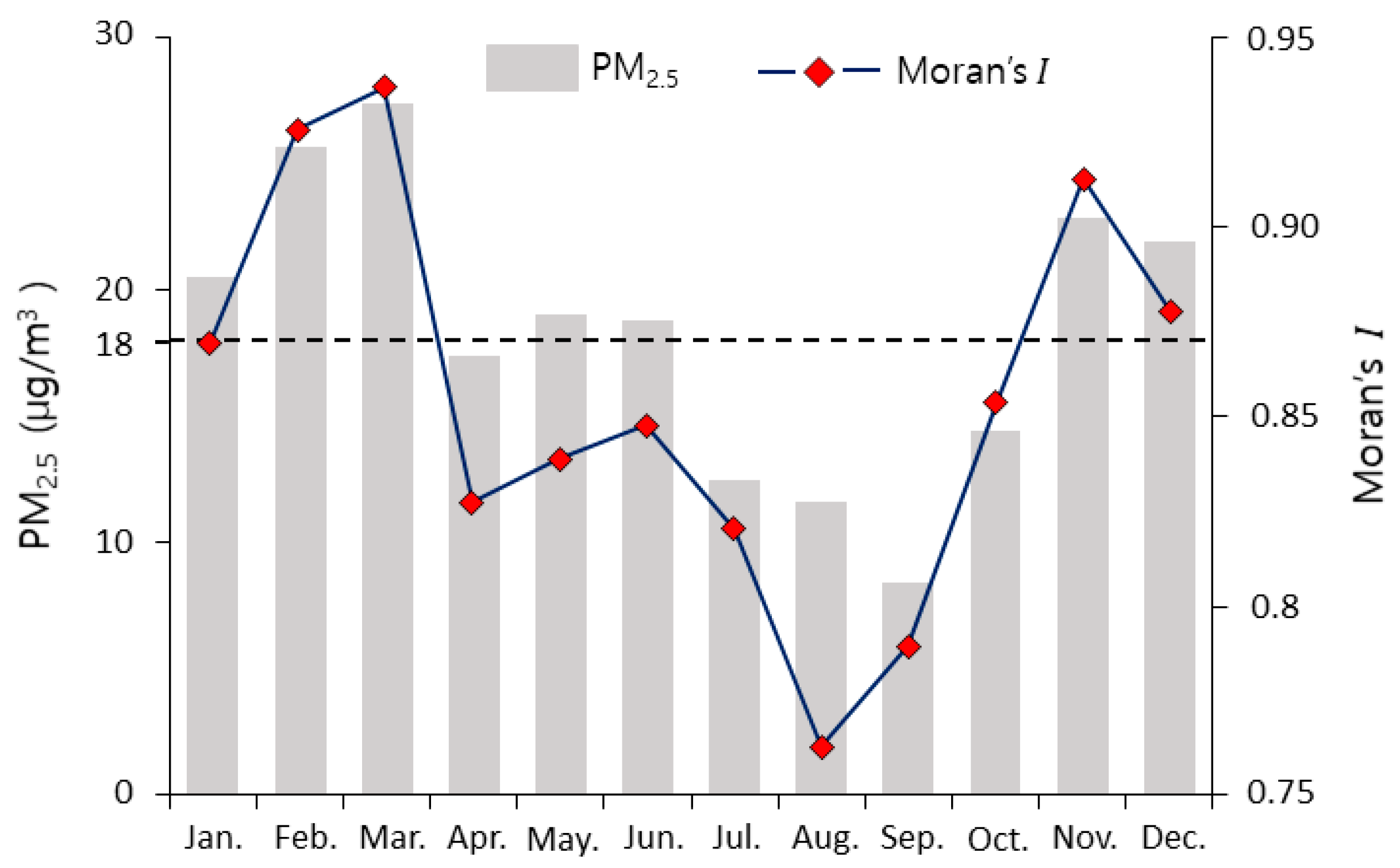
Figure 4 displays the monthly average PM_2.5 concentration and Moran’s I in 2021. The annual average PM_2.5 concentration was approximately 18 µg/m³, exceeding the Korean annual average atmospheric environmental criterion of 15 µg/m³. Additionally, the 24 h average atmospheric environmental criterion (35 µg/m³ or less) was surpassed for 29 days in 2021. The monthly average concentration was at its lowest (approximately 8.3 µg/m³) in September and peaked (27 µg/m³) in March. PM_2.5’s Moran’s I ranged from 0.76 to 0.93, significant at the 99% level, indicating spatial autocorrelation. This suggests that the PM_2.5 concentration is similar and interdependent between regions. Monthly Moran’s I and average concentration exhibited similar changes, with significant differences caused by small concentration variations as the PM_2.5 concentration decreases. In South Korea, PM_2.5 concentrations are elevated between November and March, and the concentration is high in the central region including Seoul [20]. The reason for this is that inflows, industrial complexes, high transportability, traffic volume, and heating fuels are being discussed from abroad, but it is difficult to know the exact reason. In addition, PM2.5 showed large regional characteristics, and Moran’s I showed a high value because of the characteristics of higher concentration in the central region compared to other regions.

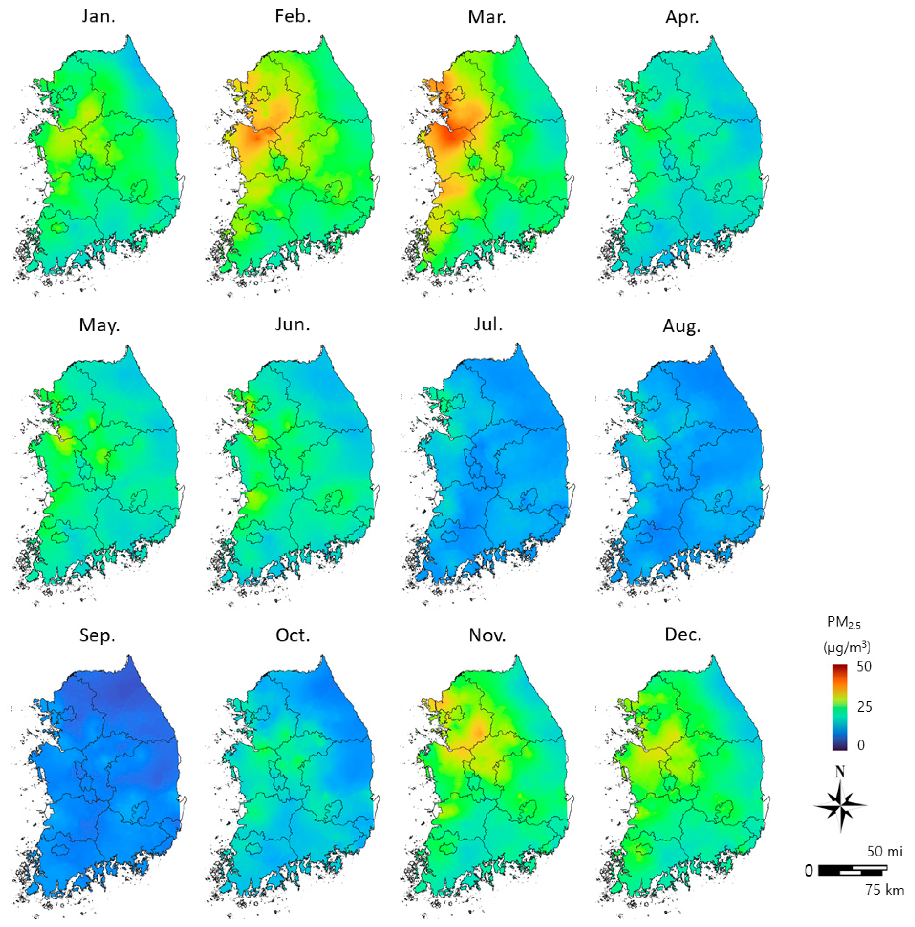
Figure 5 depicts the spatial interpolation of PM_2.5 concentration in 2021 using kriging. The concentration was relatively high in western regions, including Seoul, compared to eastern and southern regions where it was relatively low. The increase in the PM_2.5 concentration during winter is influenced by air pollutants from abroad, increased fossil fuel consumption, and the descent of the atmospheric boundary layer [21,22].

3.3. Pearson’s Correlation Analysis

In Figure 6, the monthly Pearson’s correlation analysis results between PM_2.5 and six independent variables are presented. Pearson’s correlation coefficient ranges from −1 to 1. The correlation coefficient between PM_2.5 and O₃ was highest (0.747) in July and lowest (−0.777) in November. This correlation decreased from July to November and increased from November to July. PM_2.5 and NDVI exhibited a negative correlation, with the highest value (−0.624) observed in November. The correlation between PM_2.5 and temperature mirrored O₃, reaching its peak (0.523) in September.

The correlation between PM_2.5 and humidity showed high values in January (0.427), May (0.423), and December (0.576). PM_2.5 and precipitation displayed a consistent negative correlation throughout the year, with the lowest coefficient in February (−0.555) and October (−0.506). PM_2.5 and atmospheric pressure showed a positive correlation throughout the year, with the highest coefficient (0.406) in September. The correlation coefficient of PM_2.5 and wind speed was lowest in January (−0.479) and December (−0.481), following a similar trend to O₃.

Considering the notable correlations of O₃ in July (0.747), November (−0.777), and December (−0.734), multicollinearity issues in the GWR model regression analysis are a potential concern. In previous studies, the correlation coefficient between PM2.5 and ozone was largely over 0.7, and NDVI also showed a high correlation [23,24]. While it is acknowledged that this correlation may vary over time and space, an overall strong correlation is anticipated. Among the independent variables, O₃ exhibited the highest correlation with PM_2.5, followed by NDVI, temperature, atmospheric pressure, relative humidity, precipitation, and wind speed.

3.4. Multicollinearity Analysis

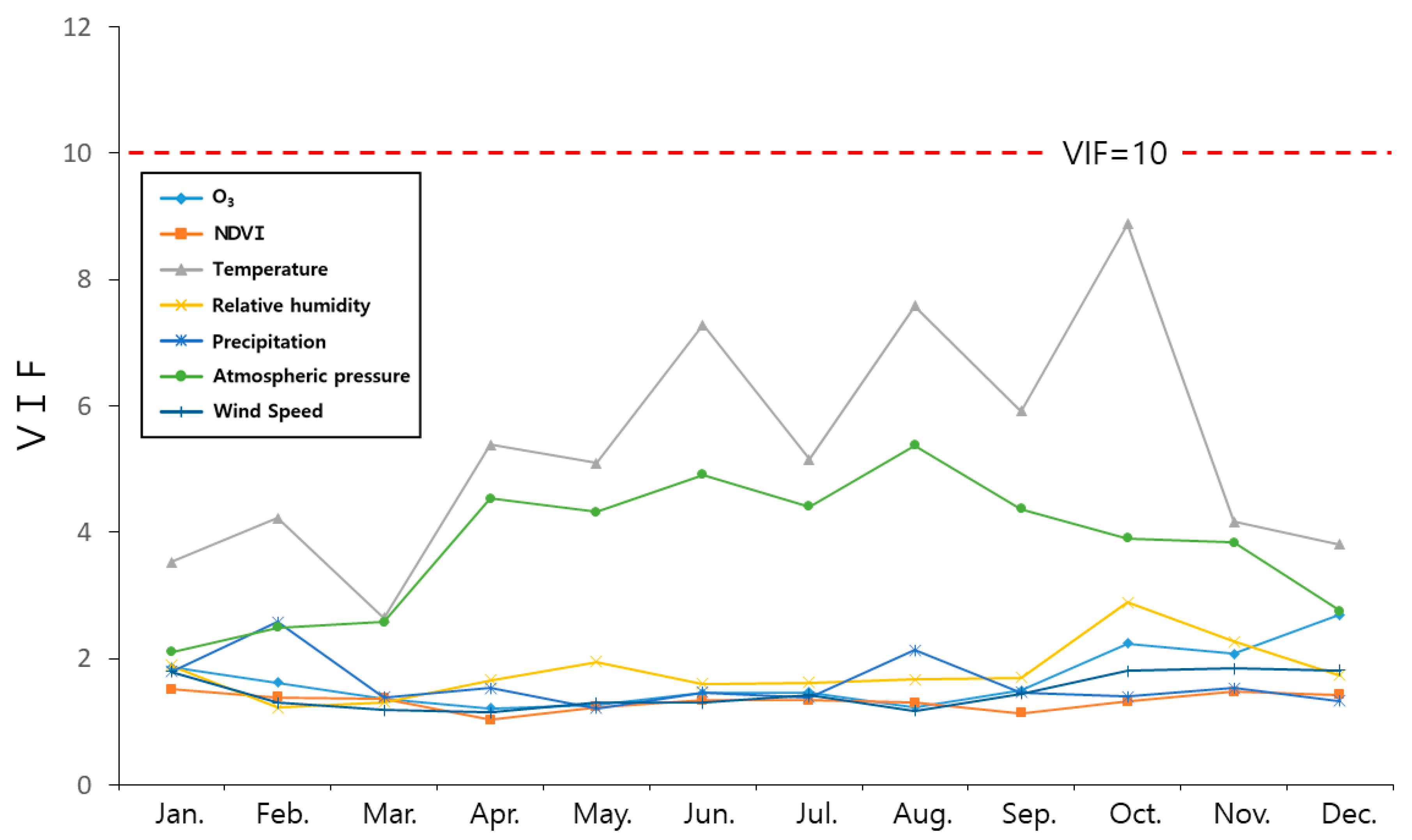
In Figure 7, the monthly VIF values for seven independent variables are presented. VIF measures the correlations between independent variables, and a value exceeding 10 indicates serious multicollinearity [18].

Among all independent variables, temperature exhibited the highest VIF, reaching a maximum of approximately 8.8 in October. Atmospheric pressure showed the next highest VIF, with a maximum value of 5.38 observed in August. The remaining independent variables maintained values below three throughout the period, indicating low multicollinearity. Although VIF was elevated for temperature and atmospheric pressure compared to other variables, it remained below 10 for all independent variables.

3.5. GWR Model Analysis

3.5.1. Analysis of the Coefficient of Determination

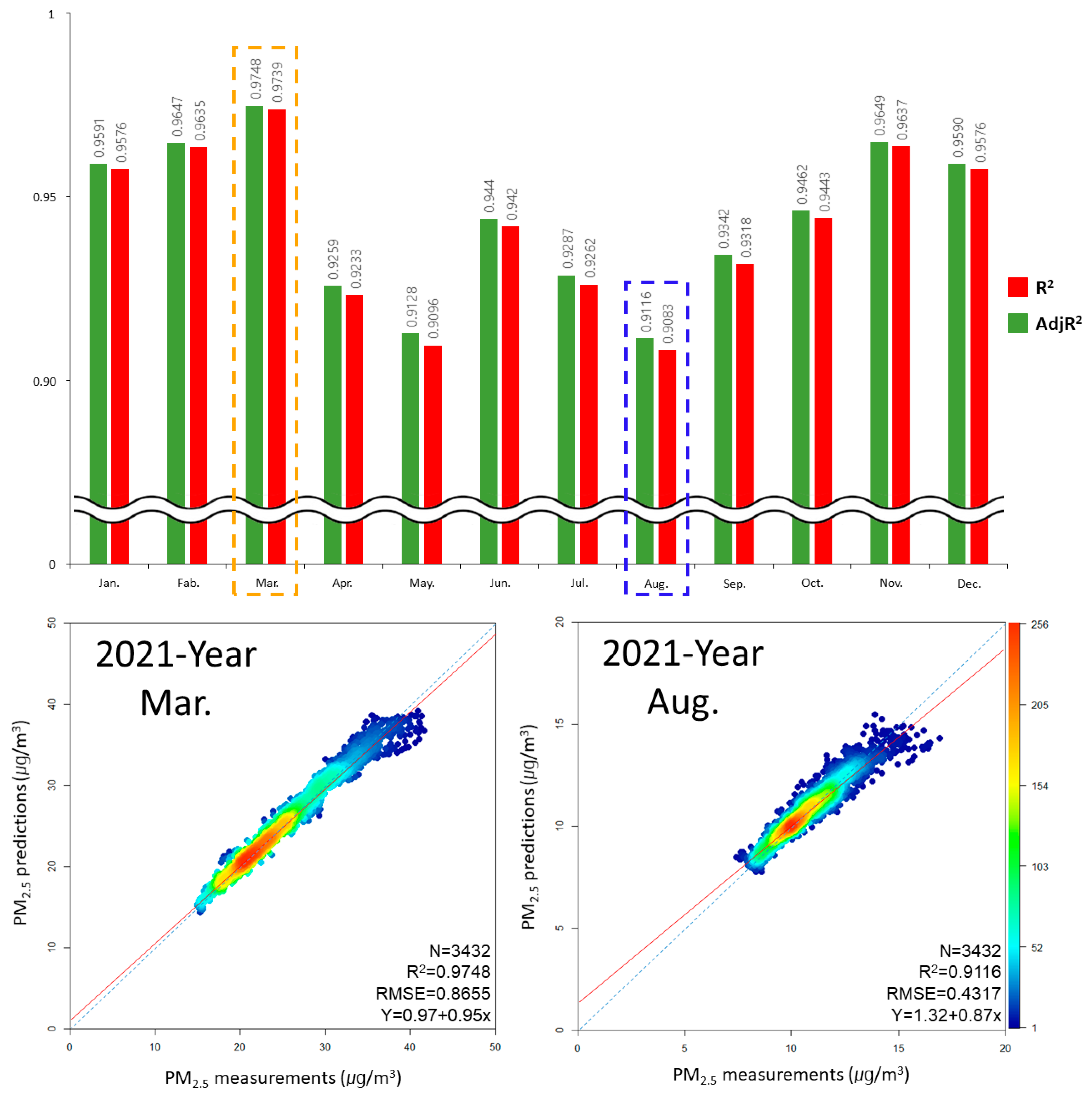
In Figure 8, the results of the coefficient of determination (R²) and adjusted-R² (AdjR²) for the GWR model are presented for the dependent variable (PM_2.5) and seven independent variables (O₃, NDVI, temperature, relative humidity, wind speed, atmospheric pressure, and precipitation), along with scatter plots for March and August. R² ranged from 0.9116 to 0.9736, and AdjR² ranged from 0.9739 to 0.9083 (Figure 8). Among the monthly results, March exhibited the highest coefficient of determination, with R² and AdjR² values of 0.9748 and 0.9739, respectively. August showed the lowest coefficient of determination, with R² and AdjR² values of 0.9116 and 0.9083, respectively (Figure 8). R² and AdjR² exceeded 0.95 from November to March, and they were relatively low from March to October (Figure 8).

To assess the model’s accuracy, R² was compared with a previous study that evaluated the suitability of the GWR model [23]. The purpose of comparing our study with previous research is to assess the reliability of the coefficient of determination produced by the GWR model we employed. The previous study introduced five GWR models: a simple GWR model, GWRK combining GWR and kriging, GWR-EBK combining GWR and EBK, GWR-TSF combining GWR and tensor spline function, and GWR-CRS combining GWR and completely regularized spline function. R² ranged from 0.662 to 0.924 for GWR, 0.893 to 0.998 for GWRK, 0.844 to 0.957 for GWR-EBK, 0.863 to 0.998 for GWR-TSF, and 0.959 to 0.999 for GWR-CRS.

In this study, the GWR model’s R² was consistently high, even though it was higher compared to GWR and GWR-EBK and lower compared to GWRK and GWR-TSF in the previous study [23]. The GWR model in this study exhibited high performance, explaining more than 90% of the total data, even without combining with other models and functions.

3.5.2. Spatiotemporal Heterogeneity Analysis

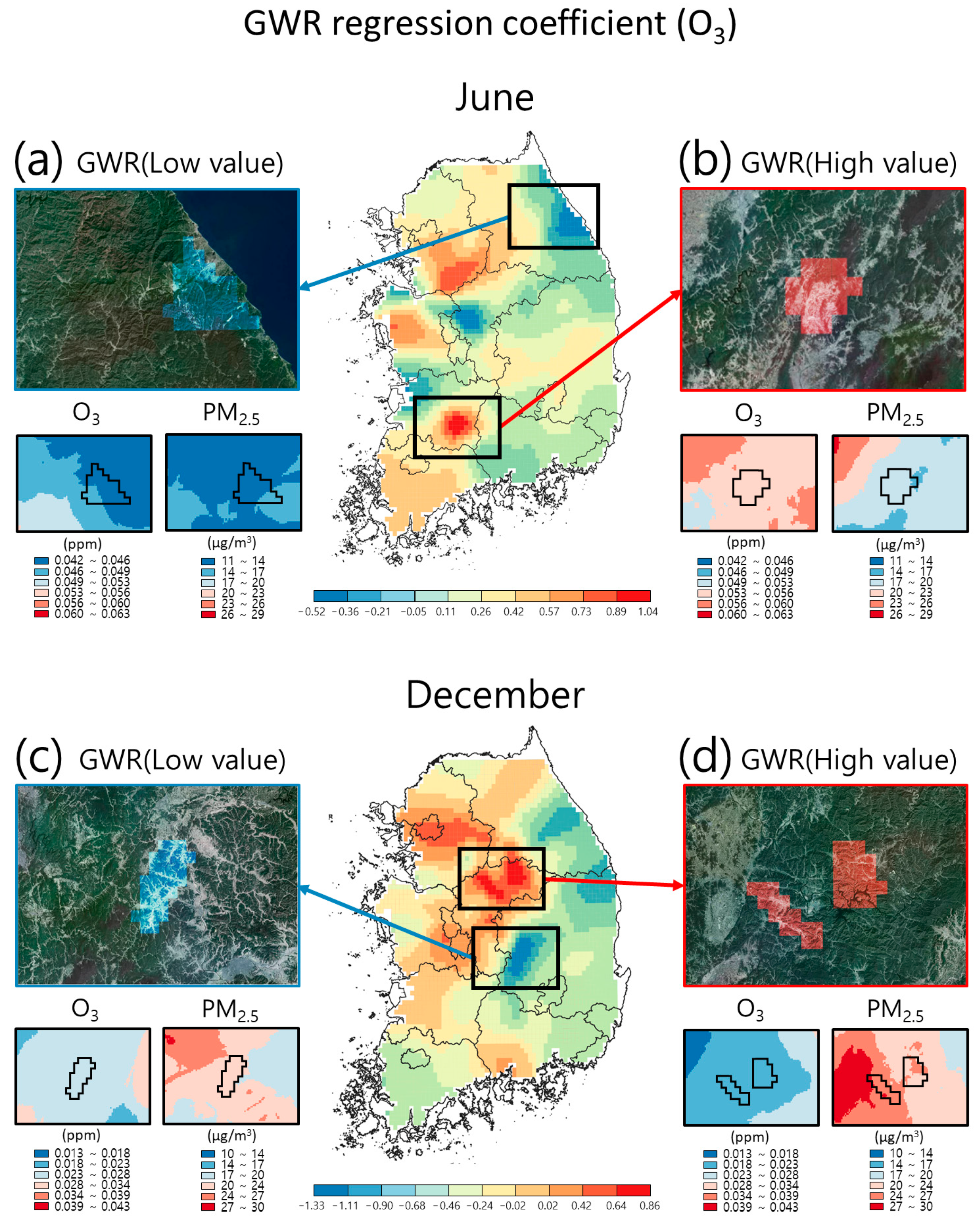
In Figure 9, the regression coefficient of O₃ from the GWR model results is presented. The analysis compares and examines the regression coefficients of PM_2.5 and O₃ for June and December, representing months with the minimum and maximum monthly average O₃ concentrations. Additionally, regions with maximum and minimum regression coefficient values are selected for detailed analysis (Figure 9).

In June, the regression coefficient of PM_2.5 and O₃ was low (approximately −0.52 to −0.36) in the eastern part of Gangwon province (Figure 9a) and high (0.89 to 1.04) in the southeastern part of Jeollabuk province (Figure 9b). In the region shown in Figure 9a, the O₃ concentration changed from 0.042–0.046 to 0.046–0.057 ppm, and the PM_2.5 concentration changed from 11–14 to 14–17 μg/m³. Notably, the O₃ concentration increased toward the left side of the region, while the PM_2.5 concentration increased toward the right side, resulting in a relatively low regression coefficient (Figure 9a). Conversely, in the region displayed in Figure 9b, the O₃ concentration decreased from 0.056–0.060 to 0.053–0.056 ppm, and the PM_2.5 concentration also decreased from 20–26 to 14–20 μg/m³. This region exhibited a relatively high regression coefficient because the concentrations of both substances decreased in the same spatial context (Figure 9b).

In December, the regression coefficient of O₃ was low (−1.33 to −1.11) in the northern part of Chungcheongbuk province (Figure 9c) and high in the western part of Gyeongsangbuk province (Figure 9d). In the region depicted in Figure 9c, the O₃ concentration increased from 0.018–0.023 to 0.023–0.028 ppm, while it decreased from 0.028–0.034 to 0.023–0.028 ppm simultaneously. Additionally, the PM_2.5 concentration increased from 17–20 to 20–24 μg/m³ and decreased from 24–27 to 20–24 μg/m³. However, the O₃ concentration was high in the northeastern and southwestern parts and low in the northwestern and southeastern parts, while the PM_2.5 concentration exhibited the opposite pattern, resulting in a low regression coefficient (Figure 9c). In the region illustrated in Figure 9d, the O₃ concentration increased from 0.018–0.023 to 0.023–0.028 ppm, and the PM_2.5 concentration increased from 20–24 to 24–27 μg/m³, leading to a high regression coefficient. Despite the opposite directions of increasing and decreasing for PM_2.5 and O₃, a high local PM_2.5 concentration in the region contributed to the observed high regression coefficient (Figure 9d).

PM_2.5 and O₃ exhibit a complex correlation, and various studies have investigated their mutual effects from diverse angles. The common cause of O₃ and secondary organic aerosol (SOA) generation lies in atmospheric oxidation reactions, with NOx and volatile organic compounds (VOCs) typically increasing together, garnering attention as contributors to both PM_2.5 and O₃ [25,26]. While previous research noted regional disparities in the correlation between O₃ and PM_2.5, with a reported low correlation in the north and high in the south [24], this study found a different pattern. In June, the regression coefficient was higher in the west and lower in the east, contrary to the north–south distinction. Korea’s topography, with higher elevations in the east and lower elevations in the west, leads to higher temperatures in the west. This topographical variation likely contributed to the observed difference in the regression coefficient of PM_2.5 and O₃.

In the west, characterized by a substantial influx of pollutants from external sources, numerous power plants, and industrial facilities, the regression coefficient of PM_2.5 and O₃ decreased from the range of −0.52 to 1.04 in June to the range of −1.33 to 0.86 in December. During winter, the atmospheric boundary layer descends, resulting in increased PM concentration due to low temperatures, while the O₃ concentration decreases due to scattered sunlight and photolysis inhibition [24,27]. This overall reduction in the regression coefficient in December, attributed to low temperatures compared to June, is indicative of the seasonal influence on the relationship between PM_2.5 and O₃ (Figure 9). The observed regional differences and seasonality in the regression coefficient are likely linked to temperature variations, solar radiation, and the distribution of air pollutants.

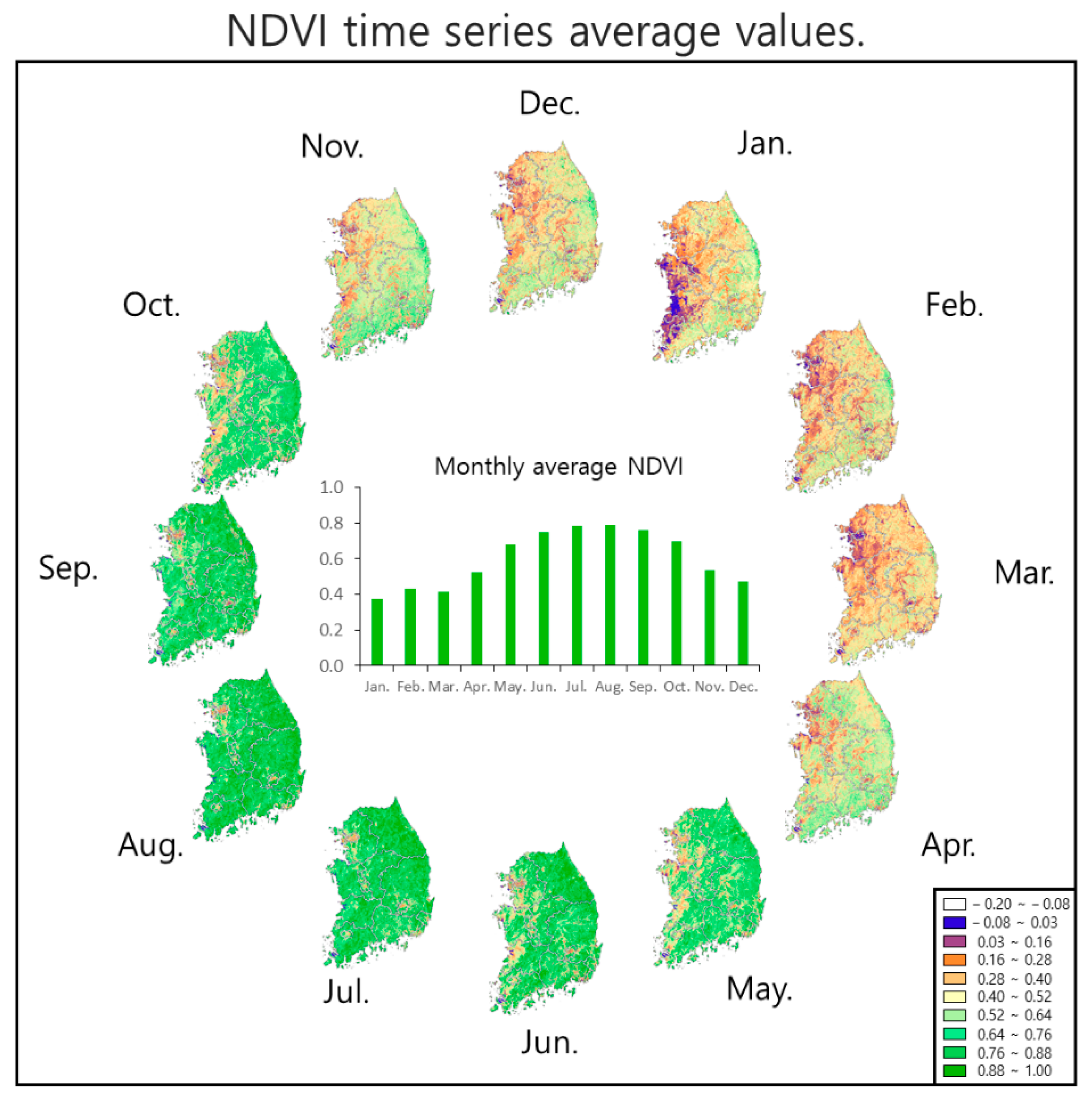
Figure 10 illustrates the monthly NDVI in 2021. August recorded the highest average NDVI (0.79) in Korea compared to other months, while January exhibited the lowest value (0.37) (Figure 10). NDVI was relatively higher in metropolitan cities than in provinces, with lower values in the west and higher values in the east (Figure 10). In January, NDVI was low (0.16 to 0.28) in the west but high (0.51 to 0.75) in certain eastern regions (Figure 10). In Korea, NDVI serves not only as a vegetation index but also as an indicator of seasonality, population distribution, and land use.

Figure 11 displays the monthly regression coefficients of PM_2.5 and NDVI from the GWR model results. The circular graph represents the ratio between positive (red) and negative (green) regression coefficients for each month. Overall, the regression coefficients of PM_2.5 and NDVI predominantly showed negative values. Specifically, at least 68% of the regions in July and up to 88% of the regions in November exhibited negative regression coefficients (Figure 11). This suggests that vegetation had a positive impact on PM_2.5 reductions in Korea.

For all periods, the regression coefficient of PM_2.5 and NDVI was notably high in the Chungcheongbuk province (Figure 11). The province, characterized as an industrial region with 95 industrial complexes as of December 2021, experiences severe air pollution due to the substantial influx of external pollutants [28]. The dense vegetation in the eastern and southern parts of the province, owing to the presence of mountain ranges, likely contributed to the elevated regression coefficient in this region, associated with increased concentrations of both PM_2.5 and NDVI. The PM_2.5 concentration might also escalate due to chemical reactions involving substances emitted from vegetation, such as BVOCs. Vegetation’s relationship with PM_2.5 is intricate, exhibiting a positive impact by generating BVOCs and participating in the formation of SOA [29,30,31] and a negative impact by adsorbing and removing PM [32,33]. NDVI, indirectly representing elevation in Korea, is likely to increase PM_2.5 concentration in the Chungcheongbuk province by interfering with air flow. Mountain ranges can induce high PM concentrations by causing atmospheric stagnation [34]. In this province, pollution accumulates in winter and spring due to wind carrying high pollution from Seoul, with surrounding mountain ranges impeding the diffusion of pollutants [28]. The relatively high regression coefficient of PM_2.5 and NDVI in the province is presumed to result from a combination of various factors.

Furthermore, a distinct difference in NDVI between the southern/eastern regions and the remaining regions is observed in November, with negative regression coefficients evident in a large area (88%) compared to other months (Figure 10 and Figure 11). The regression coefficient of PM_2.5 and NDVI is low when NDVI changes, tending to increase as NDVI rises nationwide, reducing regional differences, as seen in July and August (Figure 10 and Figure 11). For all periods, the regression coefficient is relatively low in Seoul and the Gyeonggi province (Figure 11). In these regions, NDVI covers a wide range, from low values (0.03 to 0.16) to high values (0.76 to 0.88), with noticeable changes in NDVI (Figure 10). These characteristics likely contribute to the observed low regression coefficients.

These findings affirm that alterations in vegetation exert varying effects on the PM_2.5 concentration by region, generally indicating that vegetation has a positive impact on PM_2.5 reduction.

In summary of the GWR model results, variations in the regression coefficients of PM_2.5 and O₃ in June and December were observed across regions. In June, lower coefficients were noted in the eastern part of the Gangwon province, contrasting with higher coefficients in the southeastern part of the Jeollabuk province. Conversely, in December, lower coefficients were found in the northern part of the Chungcheongbuk province, while higher coefficients were present in the western part of the Gyeongsangbuk province. These regional differences in regression coefficients are likely influenced by topographic features, weather patterns, and the locations of sources of air pollution. In the analysis of the relationship between PM_2.5 and NDVI, a generally negative regression coefficient was observed, with November displaying the largest area of negativity, indicating a positive impact of vegetation on PM_2.5 reduction. Across all periods, the regression coefficient of PM_2.5 and NDVI was notably high in the Chungcheongbuk province, suggesting intricate interactions involving industrial complexes, mountain distribution, vegetation, and air pollution in this region.

Policies addressing air pollutants have led to regional imbalances and inefficiencies. To enhance the effectiveness of pollution reduction measures, it is crucial to tailor policies to the unique characteristics of each region. In this study, a GWR model was developed, utilizing PM_2.5 in Korea as the dependent variable and O₃, NDVI, temperature, humidity, wind speed, precipitation, and atmospheric pressure as independent variables. The focus was particularly on analyzing the spatiotemporal correlations among PM_2.5, O₃, and NDVI.

The results of the analysis revealed that the monthly average concentration of O₃ was highest (approximately 0.053 ppm) in June and lowest (0.025 ppm) in December. NDVI reached its highest monthly average value (approximately 0.79) in August and its lowest (0.37) in January. Furthermore, the monthly average concentration of PM_2.5 peaked in March (27 μg/m³) and reached its lowest point in September (8.3 μg/m³), with elevated levels observed in the Seoul metropolitan area. The annual average PM_2.5 concentration was approximately 18 μg/m³, surpassing the annual average atmospheric environmental criterion (15 μg/m³) by approximately 3 μg/m³. PM_2.5’s Moran’s I ranged from 0.76 to 0.93, indicating a similarity and interdependence in PM_2.5 concentrations across regions.

In Pearson’s correlation analysis, O₃ exhibited the highest correlation with PM_2.5, followed by NDVI, temperature, atmospheric pressure, relative humidity, precipitation, and wind speed. Multicollinearity was assessed using VIF values, with no variable exceeding the critical value of 10, signifying a lack of serious multicollinearity. The GWR model demonstrated varying R² values, with the highest (0.9748) observed in March and the lowest (0.9116) in August. Comparatively, the model exhibited strong performance compared to a previous study [23].

In the GWR model, the regression coefficient of PM_2.5 and O₃ tended to be higher in the west and lower in the east, with December showing lower coefficients compared to June. These disparities are likely attributed to regional differences in precursor sources (e.g., SOx, NOx, and VOCs), temperature, and variations in solar radiation. The regression coefficient of PM_2.5 and NDVI consistently showed negative values, ranging from 68% to 88% across regions. Notably, coefficients were lower in Seoul and the Gyeonggi province but higher in the Chungcheongbuk province. This suggests that the PM_2.5 reduction effect of vegetation is more pronounced in urban areas like Seoul and the Gyeonggi province compared to suburban regions. In the Chungcheongbuk province, characterized by surrounded mountain ranges and dense vegetation, the air flow stagnation likely contributed to the high regression coefficient of PM_2.5 and NDVI. Excluding specific terrains, such as the Chungcheongbuk province, vegetation generally exhibited a positive impact on PM_2.5 reduction.

It is important to acknowledge the limitations in this study, such as errors in NDVI and insufficient measurement points. NDVI errors may arise due to cloud interference, particularly during the rainy season in summer. The choice of the inverse distance weighted (IDW) method for spatial interpolation, while potentially better for representing local features than kriging, has its drawbacks. Kriging was chosen in this study to address areas with limited measurement points, reducing errors in such regions. However, the local features captured by IDW were sacrificed. In regions with ample measurement points, employing IDW may reveal regional characteristics more accurately during spatial analysis.

4. Conclusions

GWR proves to be a valuable tool for discerning spatiotemporal correlations between PM_2.5 and various factors, showcasing its reliability. These attributes can extend beyond PM_2.5 analysis, aiding in the examination of other air pollutants and facilitating the identification of regional correlations. In the GWR regression coefficient findings, the correlation between PM_2.5 and O₃ was more pronounced in summer than in winter. This underscores the necessity for summer-specific management strategies, with a particular focus on addressing VOCs and NOx, common contributors to both PM_2.5 and O₃. Notably, the substantial impact of NDVI on PM_2.5 reduction in metropolitan areas suggests the potential for efficient PM reduction through prioritized initiatives, such as urban forest installations.

In mountainous regions, measures should be implemented to counter the phenomenon where mountain ranges intensify PM concentrations by impeding airflow. Proactive planning during urban development or strategies to enhance air flow in cities can serve as viable solutions to prevent the atmospheric stagnation induced by mountainous terrain.

Given the regional variations in air pollutants, influenced by factors, such as terrain, climate, artificial structures, and generation mechanisms, identifying the specific causes of increased pollutant concentrations in each region is crucial for public health. The study results contribute significantly to understanding regional air pollution patterns, enabling the formulation of tailored policies for effective pollution management. Emphasizing the impact of vegetation in these policies is crucial. Continuous air pollution monitoring and the development of improved prediction models are recommended for effective pollution management. The findings of this research extend beyond Korea, offering valuable insights for air pollution management in diverse geographical areas and contributing to the formulation of global policies aimed at environmental preservation and health improvement.

References

1. Brunekreef, B.; Holgate, S.T. Air pollution and health. Lancet 2002, 360, 1233–1242. [Google Scholar] [CrossRef] [PubMed]
2. Xing, Y.F.; Xu, Y.H.; Shi, M.H.; Lian, Y.X. The impact of PM2.5 on the human respiratory system. J. Thorac. Dis. 2016, 8, E69. [Google Scholar] [PubMed]
3. IARC. Air Pollution and Cancer (Scientific Publication No. 161); WHO Press: Geneva, Switzerland, 2013. [Google Scholar]
4. Calvo, A.I.; Alves, C.; Castro, A.; Pont, V.; Vicente, A.M.; Fraile, R. Research on aerosol sources and chemical composition: Past, current and emerging issues. Atmos. Res. 2013, 120–121, 1–28. [Google Scholar] [CrossRef]
5. Pacyna, E.G.; Pacyna, J.M.; Fudala, J.; Strzelecka-Jastrzab, E.; Hlawiczka, S.; Panasiuk, D.; Nitter, S.; Pregger, T.; Pfeiffer, H.; Friedrich, R. Current and future emissions of selected heavy metals to the atmosphere from anthropogenic sources in Europe. Atmos. Environ. 2007, 41, 8557–8566. [Google Scholar] [CrossRef]
6. Liousse, C.; Penner, J.E.C.; Chuang, J.; Walton, J.; Eddleman, H.; Cachier, H. A global three-dimensional model study of carbonaceous aerosols. J. Geophys. Res. Atmos. 1996, 101, 19411–19432. [Google Scholar] [CrossRef]
7. Vu, T.V.; Delgado-Saborit, J.M.; Harrison, R.M. Particle number size distributions from seven major sources and implications for source apportionment studies. Atmos. Environ. 2015, 122, 114–132. [Google Scholar] [CrossRef]
8. Tucker, W.G. An overview of PM2.5 sources and control strategies. Fuel Process Technol. 2000, 65, 379–392. [Google Scholar] [CrossRef]
9. Tomasi, C.; Lupi, A. Primary and secondary sources of atmospheric aerosol. In Atmospheric Aerosols: Life Cycles and Effects on Air Quality and Climate; Wiley: Hoboken, NJ, USA, 2017; pp. 1–86. [Google Scholar]
10. Gehrig, R.; Buchmann, B. Characterising seasonal variations and spatial distribution of ambient PM10 and PM2.5 concentrations based on long-term Swiss monitoring data. Atmos. Environ. 2003, 37, 2571–2580. [Google Scholar] [CrossRef]
11. Mei, C.L.; He, S.Y.; Fang, K.T. A note on the mixed geographically weighted regression model. J. Reg. Sci. 2004, 44, 143–157. [Google Scholar] [CrossRef]
12. Brunsdon, C.; Fotheringham, A.S.; Charlton, M.E. Geographically weighted regression: A method for exploring spatial nonstationarity. Geogr. Anal. 1996, 28, 281–298. [Google Scholar] [CrossRef]
13. Wang, L.; Zhao, B.; Zhang, Y.; Hu, H. Correlation between surface PM2.5 and O3 in eastern China during 2015–2019: Spatiotemporal variations and meteorological impacts. Atmos. Environ. 2023, 294, 119520. [Google Scholar] [CrossRef]
14. Deng, X.; Gao, F.; Liao, S.; Li, S. Unraveling the association between the built environment and air pollution from a geospatial perspective. J. Clean. Prod. 2023, 386, 135768. [Google Scholar] [CrossRef]
15. National Institute of Meteorological Sciences. 100 Years of Climate Change on the Korean Peninsula; National Institute of Meteorological Sciences: Jeju, Republic of Korea, 2018. [Google Scholar]
16. Cressie, N. The origins of kriging. Math. Geol. 1990, 22, 239–252. [Google Scholar] [CrossRef]
17. Gribov, A.; Krivoruchko, K. Empirical Bayesian kriging implementation and usage. Sci. Total Environ. 2020, 722, 137290. [Google Scholar] [CrossRef] [PubMed]
18. Craney, T.A.; Surles, J.G. Model-dependent variance inflation factor cutoff values. Qual. Eng. 2002, 14, 391–403. [Google Scholar] [CrossRef]
19. Moran, P.A. Notes on continuous stochastic phenomena. Biometrika 1950, 37, 17–23. [Google Scholar] [CrossRef] [PubMed]
20. National Istitute of Environmental Research. Annual Report of Air Quality in Korea 2020; National Istitute of Environmental Research: Inchen, Republic of Korea, 2020. [Google Scholar]
21. Cha, Y.; Song, C.K.; Jeon, K.H.; Yi, S.M. Factors affecting recent PM2.5 concentrations in China and South Korea from 2016 to 2020. Sci. Total Environ. 2023, 881, 163524. [Google Scholar] [CrossRef]
22. Kumar, N.; Park, R.J.; Jeong, J.I.; Woo, J.H.; Kim, Y.; Johnson, J.; Yarwood, G.; Kang, S.; Chun, S.; Knipping, E. Contributions of international sources to PM2.5 in South Korea. Atmos. Environ. 2021, 261, 118542. [Google Scholar] [CrossRef]
23. Wei, P.; Xie, S.; Huang, L.; Liu, L.; Cui, L.; Tang, Y.; Zhang, Y.; Meng, C.; Zhang, L. Spatial interpolation of regional PM2.5 concentrations in China during COVID-19 incorporating multivariate data. Atmos. Pollut. Res. 2023, 14, 101688. [Google Scholar] [CrossRef]
24. Zhu, J.; Chen, L.; Liao, H.; Dang, R. Correlations between PM2.5 and ozone over China and associated underlying reasons. Atmosphere 2019, 10, 352. [Google Scholar] [CrossRef]
25. Sun, J.; Wu, F.; Hu, B.; Tang, G.; Zhang, J.; Wang, Y. VOC characteristics, emissions and contributions to SOA formation during hazy episodes. Atmos. Environ. 2016, 141, 560–570. [Google Scholar] [CrossRef]
26. Zhang, J.; Wei, Y.; Fang, Z. Ozone pollution: A major health hazard worldwide. Front. Immunol. 2019, 10, 2518. [Google Scholar] [CrossRef] [PubMed]
27. Dickerson, R.R.; Kondragunta, S.; Stenchikov, G.; Civerolo, K.L.; Doddridge, B.G.; Holben, B.N. The impact of aerosols on solar ultraviolet radiation and photochemical smog. Science 1997, 278, 827–830. [Google Scholar] [CrossRef] [PubMed]
28. Allabakash, S.; Lim, S.; Chong, K.S.; Yamada, T.J. Particulate matter concentrations over South Korea: Impact of meteorology and other pollutants. Remote Sens. 2022, 14, 4849. [Google Scholar] [CrossRef]
29. Churkina, G.; Grote, R.; Butler, T.M.; Lawrence, M. Natural selection? Picking the right trees for urban greening. Environ. Sci. Policy 2015, 47, 12–17. [Google Scholar] [CrossRef]
30. Calfapietra, C.; Fares, S.; Manes, F.; Morani, A.; Sgrigna, G.; Loreto, F. Role of biogenic volatile organic compounds (BVOC) emitted by urban trees on ozone concentration in cities: A review. Environ. Pollut. 2013, 183, 71–80. [Google Scholar] [CrossRef] [PubMed]
31. Fitzky, A.C.; Sandén, H.; Karl, T.; Fares, S.; Calfapietra, C.; Grote, R.; Saunier, A.; Rewald, B. The interplay between ozone and urban vegetation—BVOC emissions, ozone deposition, and tree ecophysiology. Front. For. Glob. Chang. 2019, 2, 50. [Google Scholar] [CrossRef]
32. Lu, S.; Yang, X.; Li, S.; Chen, B.; Jiang, Y.; Wang, D.; Xu, L. Effects of plant leaf surface and different pollution levels on PM2.5 adsorption capacity. Urban For. Urban Green. 2018, 34, 64–70. [Google Scholar] [CrossRef]
33. Zenk, M.H. Heavy metal detoxification in higher plants—A review. Gene 1996, 179, 21–30. [Google Scholar] [CrossRef]
34. Chang, S.Y.; Fang, G.C.; Chou, C.C.K.; Chen, W.N. Chemical compositions and radiative properties of dust and anthropogenic air masses study in Taipei Basin, Taiwan, during spring of 2004. Atmos. Environ. 2006, 40, 7796–7809. [Google Scholar] [CrossRef]
Figure 1. (a) Geographical location and elevation profile of the study area, (b) Regional names in South Korea (yellow space represents metropolitan city, white space represents province).
Atmosphere 15 00069 g001
Figure 2. Daily variations in air pollutants and weather factors (black line represents daily average, red line represents monthly moving average). (a) O3; (b) temperature; (c) relative humidity; (d) wind speed; (e) atmospheric pressure; (f) precipitation (total daily amount).
Atmosphere 15 00069 g002
Figure 3. Histograms of each independent variable. (a) O3; (b) temperature; (c) relative humidity; (d) wind speed; (e) atmospheric pressure; (f) precipitation.
Atmosphere 15 00069 g003
Figure 4. Monthly average variation in PM2.5 and Moran’s I value for PM2.5. The annual average PM2.5 is 18 µg/m³. Moran’s I was statistically significant (p < 0.01) for all periods.
Atmosphere 15 00069 g004
Figure 5. Spatial distribution of PM2.5 in South Korea.
Atmosphere 15 00069 g005
Figure 6. Pearson’s monthly independent variable correlation. N, NDVI; T, temperature; R, relative humidity; P, precipitation; A, atmospheric pressure; W, wind speed. **: p < 0.01, *: p < 0.05.
Atmosphere 15 00069 g006
Figure 7. VIF value of monthly independent variables.
Atmosphere 15 00069 g007
Figure 8. GWR model R² and AdjR² results, March (highest R²) and August (lowest R²) scatter plots.
Atmosphere 15 00069 g008
Figure 9. June and December O3 regression coefficients of the GWR model for PM2.5. (a) Low regression coefficient in June; (b) high regression coefficient in June; (c) low regression coefficient in December; (d) high regression coefficient in December.
Atmosphere 15 00069 g009
Figure 10. Spatial distribution of monthly NDVI and average NDVI for 2021.
Atmosphere 15 00069 g010
Figure 11. Monthly regression coefficients of PM2.5 and NDVI. The central circle graph illustrates the ratio of positive and negative regression coefficients.
Atmosphere 15 00069 g011
Disclaimer/Publisher’s Note: The statements, opinions and data contained in all publications are solely those of the individual author(s) and contributor(s) and not of MDPI and/or the editor(s). MDPI and/or the editor(s) disclaim responsibility for any injury to people or property resulting from any ideas, methods, instructions or products referred to in the content.