Abstract
Drought poses a serious threat to Sudan, causing water shortages, crop failures, hunger, and conflict. The relationships between Indo-Pacific teleconnections and drought events in Sudan are examined based on the Standardized Precipitation Index (SPI), anomalies, Empirical Orthogonal Function (EOF), correlation, composite analysis, sequential Mann–Kendall test, and MK-trend test during the period of 1993–2022. The results of the SPI-1 values indicate that the extreme drought in Sudan in 2004 was an exceptional case that affected the entire region, with an SPI-1 value of −2 indicating extremely dry conditions. In addition, Sudan experienced moderate to severe drought conditions for several years (1993, 2002, 2008, 2009 and 2015). The Empirical Orthogonal Function showed that the first EOF mode (42.2%) was the dominant variability mode and had positive loading over most of the country, indicating consistent rainfall variation in the central, eastern, and western regions. Correlation analysis showed a strong significant relationship between June–September rainfall and Indian Ocean sea surface temperature (SST) (r ≤ 0.5). Furthermore, a weak positive influence of the Indian Ocean Dipole (IOD) on JJAS precipitation was observed (r ≤ 0.14). Various time lags in the range of ±12 months were examined, with the highest correlation (0.6) found at 9 month among the time lags of ±12 months. This study contributes to a better understanding of drought dynamics and provides essential information for effective drought management in Sudan. Further research is needed to explore the specific mechanisms driving these interactions and to develop tailored strategies to mitigate the impacts of drought events in the future.
1. Introduction
Kallis et al. [1] and Zhou et al. [2] stated that drought is a significant hazard resulting from the interplay between the environmental and socioeconomic systems. In meteorology, drought is commonly characterized by the extent of aridity relative to a reference point, typically an established “normal” or average level of precipitation, as well as the length of time during which the region experiences this dryness [3]. According to [4], droughts substantially threaten human activities and ecosystems, causing water resource shortages, crop failure, famine, and conflict [5,6]. Historical droughts have caused an average annual economic loss of USD 170 billion, with losses increasing to 23.125 billion dollars in 2010–2017 from 17.33 billion dollars in 1980–2009, surpassing other meteorological disaster growth rates [7,8,9,10,11,12,13,14]. Sudan (SDN) is significantly threatened by drought, a major natural hazard [15]. According to [16], the region responsible for generating 90% of the planted food crops and 85% of firewood production is approximately 69,000 square kilometers, classified as drought prone. The country experienced consecutive years of drought from 1985 to 1993, leading to significant food scarcity, social unrest, and extensive health and nutritional issues [17]. The impact of drought in SDN varies across regions, with the western region experiencing extensive impacts, the eastern and southern regions experiencing moderate impacts, and the central region experiencing less severe impacts [18,19]. Furthermore, due to the gradual progression of droughts, it can be challenging to accurately forecast their commencement and conclusion [20,21].
Numerous effects of long-distance connectivity on local and worldwide drought occurrences have been brought to light by recent research. Yin et al. [22] looked at how the El Niño Southern Oscillation (ENSO) and the Indian Ocean Dipole (IOD) work together to affect seasonal droughts across the globe. The temporal and spatial extent of these events were assessed using the Severity-Area-Duration (SAD) approach [23]. According to their study using Liang-Kleeman Information Flow (LKIF) technique [24], La Niña has a bigger influence later in life, while El Niño causes more severe droughts throughout the development and maturity periods. Compared to its cousin in the Eastern Pacific, the El Niño phenomenon in the Central Pacific has far greater effects, especially in Africa and South America. According to [25], ENSO has a major influence on the frequency of meteorological droughts, which vary greatly in terms of location and timing. Several factors, including sea surface temperatures (SST), interactions between the land and atmosphere, and ENSO, contribute to drought conditions in the Greater Horn of Africa (GHA), a region vulnerable to climatic extremes due to the confluence of natural causes and anthropogenic stressors [26,27]. The relationship between drought and ENSO events in East Africa (EA) is complex, although Kalisa et al. [28] found no evidence of a direct link between the El Niño Southern Oscillation (ENSO) and drought in the East African region. However, the association of dryness with most El Niño and La Niña years suggests that ENSO may indirectly influence drought occurrence. The authors of Doi et al. [29] predicted an imminent drought in EA, which could have adverse effects on food security, and they validated their forecast using the SINTEX-F reforecast experiments and correlation coefficients between predictions and observational/reanalysis datasets. This was investigated in 2021, with a particular focus on the ability of climate models to anticipate periods of heavy rainfall and droughts. They underscore the pivotal role of the IOD in forecasting variations in EA rainfall, which is further compounded by the ongoing process of global warming. The authors of Funk et al. [30] investigated how drought events in Africa are affected by abnormally high SSTs in the Indo-Pacific region. Their findings imply that severe El Niño occurrences, which are marked by high Western Pacific SSTs, are associated with later droughts that can be predicted and impact both Eastern and Southern Africa (EA and SA). The authors of Mahmoud et al. [31] report that during the 1970s, the Nile Basin has seen an increase in drought occurrences due to the combined impacts of amplified El Niño, intensified global warming, and IOD episodes. It is projected that this trend would continue and become stronger. The authors of Osman and Shamseldin. [32] conducted a study in SDN to investigate how rainfall patterns are affected by the SST and ENSO. It is well known that SST and warm phases of ENSO are correlated with dry conditions. The data reported by [33] demonstrate the strong correlations between anomalies in SST, ENSO, and variations in regional rainfall patterns (SDN).
Using a variety of analytical tools, such as trend analysis, the Empirical Orthogonal Function (EOF), and the Standardized Precipitation Index, this study investigates in detail the link between drought events and Indo-Pacific teleconnections in SDN. Literature on this topic is scarce. Our research aims to clarify the specific way in which drought patterns react to the impacts of climate change. The following is how this paper is organized: A thorough description of this study topic, the data collected, and the methodology employed is provided in Section 2. The results and discussion are presented and analyzed in Section 3. Section 4 serves as the conclusion.
2. Data and Methodology
2.1. Study Site Description
SDN has a total land area of over 1.87 million square kilometers and is home to approximately 33,419,625 people [34]. SDN is geographically situated in the northeastern region of the African continent, with the latitudinal coordinates of 8.686 N and 23.02 N and the longitudinal coordinates of 21.836° E and 38.6429° E (Figure 1). According to [35], SDN is surrounded by several countries. To the north, it shares its borders with Egypt. To the west, it is bound by the Chad and Central African Republic. South Sudan (SSDN) lies to the south and its eastern borders are shared by the Red Sea, Ethiopia, and Eritrea. Libya formed SDN’s northwestern boundaries.
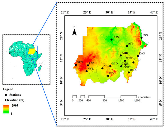
Figure 1.
The study area of Sudan showing the distribution of synoptic stations with their elevation.
2.2. Data
2.2.1. Precipitation
High-resolution (0.05° × 0.05°) precipitation records were taken from the International Research Institute (IRI) through (CHIRPS) for the period 1993–2022. ‘https://iridl.ldeo.columbia.edu/sources/.ucsb/.chirps/.v2p0/.monthly/.global/.precip/’ (Accessed on 23 November 2022). CHIRPS is a cutting-edge daily observational dataset designed to monitor droughts in EA [36]. The authors of de Waal. [37] stated that the recent conflict in distinct parts of the country and the lack of essential services made it difficult for conventional ground-based stations to spread throughout SDN. Because of its ability to combine information from satellites and ground-based observations, CHIRPS data are superior for tracking rainfall variability and extreme occurrences such as droughts [35]. These findings suggest that their use should be promoted in regions with a limited number of weather stations.
2.2.2. Wind and Mean Sea Level Pressure (MSLP)
The wind components at altitudes of 200, 500, and 850 hPa, as well as the MSLP, were analyzed using data with a resolution of 0.25° × 0.25°. This analysis was conducted to investigate the atmospheric conditions that contribute to persistent concordant droughts, and the wind anomaly patterns were evaluated during these periods of drying. The data used for this analysis were obtained from the European Center for Medium-Range Weather Forecasts (ECMWF) and can be accessed through the following link: https://Cds.Climate.Copernicus.Eu/Cdsapp#!/Dataset/Reanalysis-Era5-Single-Levels?Tab=Form, (accessed on 24 December 2022).
2.3. Methods
2.3.1. Climatic Indices
In this study, the NINO 3.4 sea surface temperature (SST) anomaly was calculated as the difference between the current SST and the three-month moving average for the region situated between 5° N and 5° S latitude and 170° W and 120° W longitude to represent ENSO conditions. The Oceanic Niño Index (ONI) was used to classify ENSO phases based on the rules set by the National Oceanic and Atmospheric Administration (NOAA). Specifically, three months in a row of ONI values above a threshold of +0.5 °C were considered signs of El Niño event, and three months in a row of ONI values below a threshold of −0.5 °C were considered signs of a La Niña event. The neutral phase remained within this range [38]. The data for this study were obtained from the NOAA website: ‘[https://psl.noaa.gov/gcos_wgsp/Timeseries/Nino34/]’ (accessed on 23 November 2022).
For the IOD, the authors calculated the differences in temperature conditions between the western equatorial Indian Ocean (50° E–70 °E and 10° S–10° N) and the southeastern Indian Ocean (90° E–110° E and 10° S–0° N) within the equatorial region of the Indian Ocean resulted in the Indian Ocean Dipole Mode Index (DMI) (Molla 2020). The DMI is a crucial metric for the detection and characterization of IOD [39]. The IOD enters a positive phase when the DMI values are greater than +0.4 °C, whereas it is considered a negative phase when the DMI drops below −0.4 °C. The IOD is in a neutral state when the DMI values range from −0.4 °C to +0.4 °C. Information regarding the DMI was obtained from the following website: https://psl.noaa.gov/data/timeseries/DMI (accessed on 23 November 2022).
2.3.2. The Standardized Precipitation Index (SPI)
The SPI is a globally recognized indicator that is employed to ascertain and categorize meteorological drought occurrences. The SPI indicator, formulated by [40] and extensively elucidated by [41], is a quantitative measure of rainfall anomalies at a specific geographical point. The SPI is calculated by contrasting the observed cumulative precipitation values over a specified accumulation period with the historical rainfall data for the same period. This methodology is outlined in detail in references [42,43,44]. The transformation of raw precipitation data is a fundamental aspect of the SPI methodology, as it requires the observed precipitation to be fitted to a probability distribution. Precipitation data frequently exhibit a skewed distribution, which the Gamma distribution is an effective model for. The cumulative distribution function (CDF) of observed precipitation is calculated and transformed into a standard normal distribution to calculate the SPI. The transformation process standardizes precipitation data. A positive value indicates above-median precipitation, while a negative value indicates below-median precipitation. This index quantifies the number of standard deviations above or below the average, offering a transparent and uniform method for evaluating precipitation anomalies. The SPI possesses several advantages over alternative statistical tools, including its emphasis on precipitation as the primary driver of drought [45,46,47]. The equation of the SPI:
where denotes the standard deviation, is the long-term mean, and is the observed value.
2.3.3. Anomaly
This refers to a deviation from the average value of a variable, which can be either negative or positive, highlighting that the actual value of the variable is either higher or lower than the anticipated or expected value, respectively [48]. The arithmetic anomaly was calculated using the following formula:
where is an anomaly, is the observation value, and it is the mean value.
2.3.4. The Empirical Orthogonal Function (EOF)
This method decomposes a dataset into a set of orthogonal (i.e., independent) functions. In climate studies, EOFs often represent spatial variability modes [49]. This technique has been widely applied in spatiotemporal drought studies [50]. In this study, EOFs were used to analyze and obtain the dominant spatial and temporal patterns of drought variability in SDN. The EOF approach is used to analyze the variability of a single field by identifying temporal and spatial patterns and determining the significance of each pattern [51]. In this study, time series are referred to as principal components (PCs) and spatial patterns are referred to as EOFs. The EOFs were computed using the following formula:
where is the space- and time-distributed data field and and are the matrices of the eigenvectors and eigenvalues, respectively.
2.3.5. Pearson’s Correlation Coefficient (PCC)
PCC is a statistical metric used to evaluate the linear correlation between two elements [48,52]. Furthermore, the relationship strength is enhanced as it approaches values closer to −1 are correlated negatively, whereas values closer to 1 are positively correlated. However, this weakens as approaches zero. This indicates that the predictor variables can explain the variations observed in the response variables with few errors. The authors of Mclean et al. [53] established a direct association between the magnitude of the correlation coefficient (CC) and the inaccuracy level. Researchers [54,55,56,57,58] applied the PCC approach to investigate the relationship between weather variables and droughts in the GHA. This study used a correlation analysis to measure the relationships between IOD, ENSO and SDN precipitation. To obtain the CC, this method employs regression analysis of the connection between x and y.
Pearson’s correlation coefficient (R)
where the PCC, denoted as , measures the direction and strength of the linear relationship, between two variables . This is computed by dividing the covariance of and by the product of their deviations and . Limits of −1 and 1 were calculated using the PCC. Degrees of freedom were used to determine statistical significance using the t-test.
2.3.6. Composite Analysis (CA)
The objective of this research is to examine the significant impact of atmospheric circulation on meteorological variability, specifically wind variability and MSLP, using CA, which is a crucial methodology in the field of meteorology. CA involves calculating the average value of specific variable categories, which are chosen based on their correlation to important conditions. It is essential for the CA to have arid conditions. The first step involved selecting the above-mentioned years (1993, 2002, 2004, 2008, 2009 and 2015) based on the SPI, which indicated the occurrence of droughts in these years. The selected events were then averaged. The resulting averaged events were then subtracted from the average of the non-events, forming the CA [59]. The results of CA are used to formulate hypotheses about patterns related to atmospheric circulation, with the aim of detecting anomalies in the circulation of wet and dry events.
2.3.7. Trend Analysis
(a) Sequential Mann–Kendal trend analysis (SQMK)
It is a statistical method used to analyze the trends and significance of sequential data. The SQMK method was used to show a sudden change in the trend or an estimate of the year in which the important trend started during the study period. It is also used to check for trends in sequential data [60]. This study used analysis to investigate the occurrence of drought in the time series of seasonal JJAS and yearly precipitation. The analysis entailed illustrating the progressive function u(t) and backward function u’(t) throughout the investigation. According to [61], variable U(t) is a standardized variable with a mean of zero. The intersection or divergence of the progressive and backward functions beyond a certain threshold result in a top confidence limit of +1.96 and a lower limit of −1.96 for a 95% confidence level [62].
(b) Mann–Kendal test
It is a widely used nonparametric method for detecting trends in meteorological time series, such as drought indicators [63,64,65]. This test assesses whether there is a significant upward or downward trend in time-series data [66], making it ideal for long-term research as recommended by the World Meteorological Organization (WMO). The null hypothesis (H0) posits no trend, while the alternative hypothesis (H) suggests a monotonic trend. The significance of the trend is determined through the Z-statistic and p-value [45]. The MK test was formulated as follows:
where xj is the sequential data value and n is the length of the dataset.
Statistical distribution S approaches normality when n ≥ 8. The variance and mean are calculated using the subsequent formulas:
where tm denotes the extent m. \to calculate the standardized test statistic, Z was computed using the following equation:
At the significance levels of 0.01, 0.05, and 0.1, |Zα| was 2.58, 1.96, and 1.65, respectively.
3. Results and Discussion
3.1. The Standardized Precipitation Index (SPI)
Temporal progression of the SPI for SDN’s area was averaged over the period 1993–2022. The patterns of arid and moisture development in this region are depicted in Figure 2. Figure 2a illustrates that notable drought occurrences transpired in 2002, 2004, 2008, and 2009 throughout this period. 2004 was notably a remarkably arid year (SPI ≤ −2), as evidenced by SPI-1. However, as illustrated in Figure 2b, significant drought occurrences transpired in the years 1993, 2002, 2004, 2008, 2009, and 2015. Notable drought years in SPI-1 included 2008 and 2009 (SPI ≤ −1.5), and 2004 was an extreme dry year (SPI ≤ −2). It was surprising that drought did not occur during the annual rainfall in 1993, while it occurred during the rainy season JJAS. We found that the SPI represented a persistent challenge for SDN over these 30 years, with frequent and persistent drought conditions. These findings are aligned with the classification system proposed by [28,46,47] for the SPI, which underscores the severity and long-lasting impacts of these drought events in SDN These findings are also aligned with those of prior investigations conducted by [67,68], which emphasized the recurrent and prolonged nature of drought events in SDN. This pattern of climatic stresses highlights the importance of proactive drought management and resilience planning for SDN’s future.
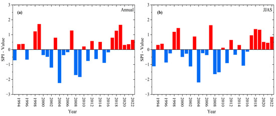
Figure 2.
Temporal variation in SPI-1 for (a,b) annual and JJAS precipitation over Sudan from 1993 to 2022. Calculated based on precipitation from the CHIRPS. This figure shows the changes in these indices over time.
3.2. Anomaly
The areas marked in white on the map, especially the northern one, have a striking lack of rainfall. This indicates that there was minimal to no rainfall at these locations throughout the observation period due to the prevailing dry meteorological conditions.
Figure 3a shows the long-term spatial mean of precipitation compared to (b–g) drought events that occurred over six years (1993, 2002, 2004, 2008, 2009, and 2015). Figure 3b depicts JJAS precipitation in SDN in 1993, revealing that the northern region of the country, including Khartoum (KH), Aljazirah (AJ), North Kordfan (NK), North Darfur (ND), East Darfur (ED), and South Darfur, was severely affected by drought. Figure 3c illustrates the JJAS precipitation in 2002, indicating that the northern region of the country, including KH, AJ, White Nile (WN), NK, and ND and South Darfur, was highly affected by drought. Figure 3d displays the JJAS precipitation in 2004, showing that the entire region was affected by drought, with the Blue Nile (BN) and West Kordfan (WK) being more severely affected, whereas West, Central, and South Darfur were unaffected. Figure 3e illustrates the JJAS precipitation in 2008, revealing that the entire region was affected by aridity, with a significant impact on southern and northern Darfur. Figure 3f shows JJAS precipitation in 2009, indicating that Gedaref (GD), Sennar (SN), BN, and West Darfur (WD) were affected by drought. Figure 3g depicts the JJAS precipitation in 2015, revealing that NK, ND, KH, Kassala (KS), AJ, and WN were highly affected by drought. The comparison shows that the rainfall was less extended over the SDN map, which represents the spatial coverage of the JJAS precipitation for these six years compared with the total annual mean precipitation (1993–2022). Our results support the findings of [15,67], which emphasize the recurring and prolonged nature of drought events in SDN, especially in ND. However, these results highlight the region’s vulnerability to climate change, the importance of long-term meteorological data to understand climate dynamics, and the urgent need for region-specific climate adaptation strategies.
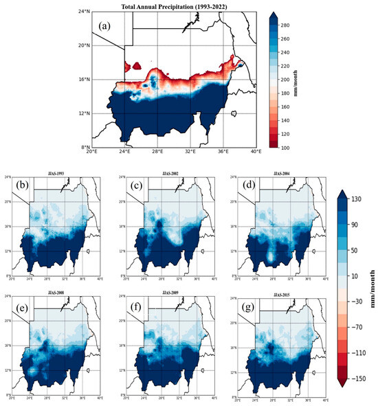
Figure 3.
(a) Total Annual Mean of Precipitation for 1993–2022 comparing with six drought events (b–g) in Sudan for 1993, 2002, 2004, 2008, 2009, and 2015.
3.3. Trend
A brief synopsis of the Sequential Mann–Kendall (SQMK) analysis was performed using the Mann–Kendall test in Table 1. The JJAS and annual rainfall trends from SDN 1993 to 2022 were graphically illustrated using the SQMK analysis (Figure 4a,b). The JJAS progressive and retrograde lines crossed in 2016, and as the period ended, the progressive rainfall levels increased steadily. The progressive and retrograde lines for annual rainfall crossed in 2016, after which both lines exhibited a steady increase, until the end of the time series. The intersection between the progressive and retrogressive functions (2016) represents the mutual point of the abrupt change in rainfall, from decline to increase. 2016 represents the mutual point in rainfall and divides the time series into two periods, i.e., 1993–2016 (decreasing period) and 2016–2022 (increasing period). The comprehensive results show that the annual and JJAS rainfall has an increasing rainfall trend after 2016 (mutual point); however, the annual rainfall shows more abrupt changes. At the 95% confidence level, the changes were found to be statistically significant for the annual case, while, at the 5% confidence level, they were not significant for the JJAS case. The intersection points in 2016 showed a sharp decrease in JJAS rainfall and rise in SDN’s annual rainfall, reversing the previous decades-long decline in rainfall. The outcomes of this study are inconsistent with those of [33], who reported a substantial increase in annual and JJAS rainfall in SDN. Furthermore, [69,70] documented that increased rainfall variability in EA leads to more extreme weather events. Nevertheless, our study only demonstrated statistical significance regarding the annual precipitation pattern and the reduction in the prolonged decline in Sudan rainfall. The results appear to indicate a reversal of the long-term rainfall decline in SDN, with a notable increase in precipitation in recent years. This is a matter of significant concern, as the reduction is likely to have a detrimental impact on the national economy of SDN, as the majority of agricultural activities are sustained by the July to September rainfall season over SDN. If the observed trend is implemented, it would provide a much-needed economic boost to the region.

Table 1.
The JJAS and annual rainfall trend test over Sudan were summarized using the Mann–Kendall test at the 95% confidence level.
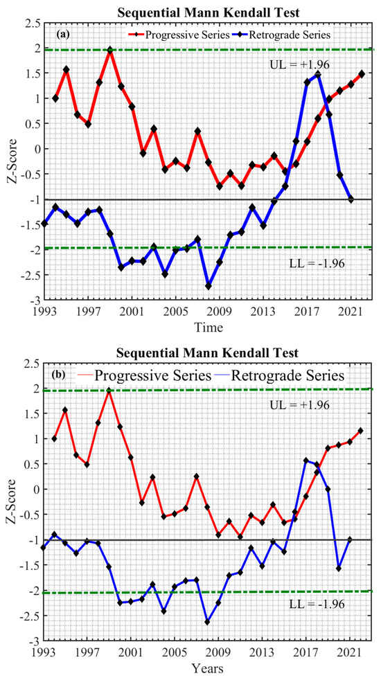
Figure 4.
Sequential Mann–Kendall analysis for rainfall derived from CHIRPS for (a) JJAS and (b) annual rainfall over Sudan during 1993–2022. The upper limit (UL) and lower limit (LL) dashed lines represent confidence limits at α = 5%.
3.4. The Empirical Orthogonal Function (EOF)
In this study, the EOF analysis was employed to examine the dominant mode of variability in the June to July (JJAS) rainfall over the region of interest. Figure 5. depicts the spatial modes and corresponding Principal Components (PCs) of the three initial EOF modes. The cumulative variances accounted for by the three initial EOF modes are 42.2%, 13.6%, and 8.8%, respectively. The first EOF mode (EOF-1) demonstrated positive loading as the dominant variability mode (Figure 5a) across most of the country, indicating consistent rainfall variation in these areas. This suggests that the central, eastern, and western regions were more prone to anomalous wet conditions than the rest of the study area during the JJAS. The second and third EOF modes accounted for 22.4% of the total variance during the JJAS rainfall season (Figure 5b,c). The results of EOF-2 revealed two spatially distinct areas of drought variability in the south and west of the country during the study period (Figure 5b). EOF-3 showed negative loadings over the northern, eastern, and western corners and their hinterlands, whereas the remaining areas exhibited positive loadings (Figure 5c). Considering the outcomes obtained from the dominant mode (i.e., EOF1), amplitudes greater than one standard deviation were observed in 1998, 1999, 2007, 2017, and 2018. Similarly, amplitudes less than minus one were observed in 1996, 1997, 2000, 2001, 2002, 2011, 2013, and 2015. These years were used in the CA to identify potential circulation anomalies that were likely associated with anomalous wet and dry conditions during the study period. These findings align with those of [71], who discovered that EOF-1 is the dominant mode for all seasons, reflecting the primary seasonal precipitation pattern in Africa. This is in contrast with the claims made by [35] regarding the drought-prone regions of SDN, particularly in the west and south, where EOF-2 is suggested to differ. EOF-3 further revealed that certain areas exhibited positive loadings, whereas the northern, eastern, and western regions and their surrounding areas experienced negative loadings. However, it is imperative to note that the scope of these findings was constrained by data availability and provide important information and a comprehensive understanding of the spatiotemporal variability of JJAS precipitation in SDN for regional water resources management, agriculture, and environmental planning.
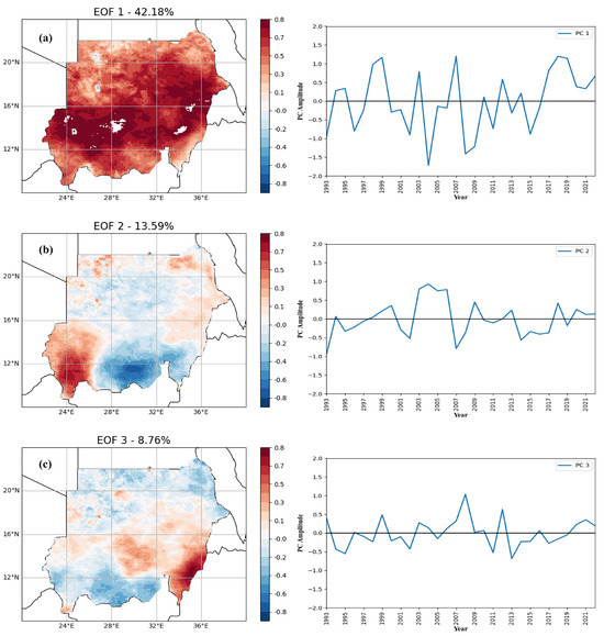
Figure 5.
The first three modes for the JJAS rainfall showing spatial distribution (left) and their corresponding principal components (right) for (a) EOF1, (b) EOF2, and (c) EOF3, over SDN based on CHIRPs gridded data from 1993 to 2022.
3.5. The Linkage with Indo-Pacific Oceans Temperatures
The outcomes of the spatial correlation analysis in Figure 6a indicate a significant positive relationship with the correlation coefficient (CC) of (r ≤ 0.50) between the JJAS rainfall and the Nino 3.4 index in SDN’s northern, eastern, and western regions. However, other areas are significantly negative, highlighting the spatial influence of the Nino 3.4 index on SDN’s precipitation patterns during the period 1993–2022. Figure 6b shows a relatively negative relationship with CC of (r ≤ −0.40) between the IOD index and the JJAS rainfall in the north and south and weak positive correlation in the western and eastern part of the area, demonstrating the spatial impact of the IOD index on rainfall patterns across SDN. Figure 6c shows that a correlation from 1993 to 2022 is significant and includes the driest period in SDN. This relationship is evident in both El Niño years (1993, 1997, 2002, 2015 and 2019) and La Niña years (1999, 2000, 2007, 2008, 2011, 2021 and 2022). In contrast, Figure 6d shows a relatively weak positive association between the IOD index and precipitation during JJAS. There was a clear relationship between precipitation and both a positive IOD (1994, 1997, 2012 and 2019) and a negative IOD (1996, 2005, 2007 and 2016).
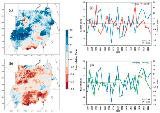
Figure 6.
Spatial and temporal correlation between JJAS rainfall and the Nino 3.4 Index (a,c), and JJAS rainfall and the IOD index (b,d). (The correlation is statistically significant at the 95% confidence level, shown as black dots.)
The rise of Nino 3.4, a neutral case, would occur within three months of January, according to Figure 7a, which illustrates the highest cross-correlation of 0.3 with a three-month lag. Consequently, January showed a drop in precipitation. As shown in Figure 7b, the increase from Nino 3.4, a neutral case, would happen within a year of February based on the highest cross-correlation of 0.4, which indicates a lag of-12 months. February presented less rainfall as a result of this. At a lag of 1 month, Figure 7c demonstrates that the highest cross-correlation of 0.4 indicates that the increase in Nino 3.4 would happen no later than one month prior to March. March’s precipitation decreased consequently. The correlation between Nino 3.4 and precipitation in Figure 7d is −0.5, with a lag of 8 months. This indicates that the optimal time shifts for these variables happen when Nino 3.4 declines about eight months before precipitation increases in April. Figure 7e exhibits the highest correlation of −0.5 at a lag of −7 months, suggesting that the best time shifts for the variables Nino 3.4 and rainfall happen when Nino 3.4 decreases coincide with an increase in precipitation approximately seven months after May, which precedes increased May rainfall. According to Figure 7f, the highest correlation of −0.4 indicates that, at lags of −3 and −4 months, the decline in Nino 3.4 occurs three to four months before an increase in precipitation, leading to an increase in rainfall in June. Relative to zero months, Figure 7g displays a correlation of −0.4. It can be concluded from this that an increase in precipitation in approximately the same months precedes the decrease in Nino 3.4, consequently increasing precipitation in July. With zero months of lag, Figure 7h displays a correlation of −0.4. This suggests that an increase in precipitation around the same month precedes the decline in Nino 3.4, meaning that August will see an increase in precipitation. The highest 0.6 correlation is seen in Figure 7i at lags of nine months, indicating that the optimal time lags for the variables Nino 3.4 and rainfall occur when Nino 3.4 increases after precipitation decreases by approximately nine months, with September being the month before and September experiencing a decrease in precipitation. According to Figure 7j, the best time shifts for the variable’s precipitation and Nino 3.4 happen when there is a lag of one month between the highest correlation of −0.4. From this, it can be inferred that October experiences less precipitation since the increase in Nino 3.4 occurs approximately one month ahead of the precipitation decrease. As can be found in Figure 7k, the greatest correlation between 0.4 and precipitation occurs when there is a three-month lag between an increase in Nino 3.4 and a decrease in precipitation, which in turn results in less precipitation in November preceding the increase in Nino 3.4 by approximately three months. As shown in Figure 7l, the greatest correlation 0.3 between Nino 3.4 and precipitation occur at zero-month lag. This means that the best time lags for Nino 3.4 and precipitation occur when an increase in Nino 3.4 corresponds to a decline in precipitation before approximately zero months, resulting in a decrease in precipitation in December.
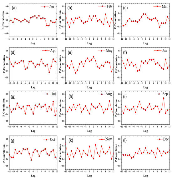
Figure 7.
The cross-correlation between Sudan’s rainfall and the Nino 3.4 teleconnection from 1993 to 2022.
The strongest correlation, 0.4, between the IOD and precipitation variables is seen in Figure 8a,b. This correlation has a time lag of zero months, indicating that an increase in IOD occurs approximately one month ahead of a decrease in precipitation. This indicates that January and February would observe less rainfall due to an increase in IOD this month. The greatest cross-correlation of 0.4 between the precipitation and IOD variables is shown in Figure 8c. This cross-correlation happens five months after March, causing a reduction in precipitation in that month. With a lag of three months, Figure 8d Shows the highest correlation of 0.4 between the variables IOD and precipitation. This suggests that a decrease in precipitation in April is caused by a decrease in IOD approximately three months prior to the latter. With a one-month time lag, Figure 8e displays the highest correlation (0.4) between the variables IOD and precipitation. This proposes that a decrease in precipitation in May is caused by an increase in IOD that occurs approximately one month after a decrease in precipitation. With a two-month time lag, Figure 8f shows the highest correlation (0.4) between the variables IOD and precipitation. This implies that precipitation will decrease in June due to a decrease in precipitation occurring approximately two months earlier due to an increase in IOD. With a lag of four months, Figure 8g displays the highest correlation −0.6 between the variables IOD and precipitation. This implies that precipitation increases in July are caused by a decrease in IOD approximately four months in advance of the precipitation increase. With a 5-month time lag, Figure 8h shows the highest correlation of 0.5 between the variables IOD and precipitation. This suggests that a rise in IOD occurs approximately five months prior to a fall in precipitation, resulting in a fall in precipitation in August. With a 9-month time lag, Figure 8i displays the highest correlation of 0.5 between the variables IOD and precipitation. The implication is that precipitation decreases in September because an increase in IOD occurs about nine months after September, when precipitation decreases. Figure 8j shows the highest correlation of −0.4 between the variables IOD and precipitation, which occurs with a time lag of −6 months. This suggests that a decrease in IOD precedes an increase in precipitation about six months before October, leading to an increase in precipitation in October. Figure 8k displays the highest correlation of 0.5 between the variables IOD and precipitation, which occurs with a time lag of zero months. This indicates that there would be an increase in IOD this month, leading to a decline in rainfall in November. With a three-month time lag, Figure 8l displays the highest correlation of 0.3 between the variables IOD and precipitation. This implies that an increase in IOD precedes a decrease in precipitation by about three months after December, leading to an increase in precipitation in December.
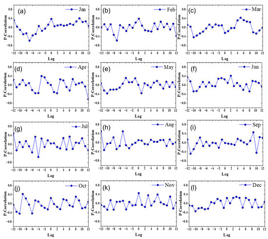
Figure 8.
The cross-correlation between Sudan’s rainfall and the IOD teleconnection from 1993 to 2022.
Most importantly, we demonstrated strong/weak positive correlation between ENSO, IOD, and drought occurrences in SDN, with significant impacts on precipitation levels. Our findings align with recent studies conducted in EA by [72,73], affirming that El Niño has substantial effect on reducing precipitation levels in the region. Similarly, [31] and [74] also found evidence of El Niño’s influence in decreasing rainfall in SDN. However, our results contradict the report by [57,75], which suggests that a positive IOD increases precipitation in southern EA, which could be attributed to the difference in the rainy season patterns (i.e., bimodal rainfall pattern, the short rainy season (March to May) and the long rainy season (October to December)) or triggered by other atmospheric drivers such as Madden-Julian Oscillation (MJO) [76]. The present findings contribute to the existing knowledge on the influence of climate indices, such as Nino 3.4 and IOD, on precipitation variability. This understanding is crucial in the context of climate change, as it can worsen extreme weather events. Therefore, comprehending these dynamics is important for accurate precipitation forecasting and effective water resource management in the region.
3.6. Composite Analysis
(a) Wind circulation:
During dry periods, SDN is marked by dominant and intense south-westerly winds at 200 hPa, as depicted in Figure 9a. This altitude hosts the Tropical Easterly Jet (TEJ), ranging between 200 and 100 hPa [77], which can either suppress or enhance convective activities through its effects on upper-level convergence and divergence. Originating near the Maritime Continent (MC), the TEJ extends towards northern Africa and diminishes rapidly as it traverses SDN [78]. The precipitation dynamics in SDN are affected by the interplay between the TEJ’s proximity to the surface-level Intertropical Convergence Zone (ITCZ), the occurrence of wave patterns within the TEJ flow, and the variability in moisture delivery to the region. During dry spells, a notably weaker TEJ is observed veering southwards across SDN [79]. In contrast, the influence of the African Easterly Jet (AEJ) is significant during these periods, identifiable at the 500 hPa level with distinctive north-easterly and south-westerly wind patterns in SDN, as illustrated in Figure 9b. The AEJ, stretching from the Arabian Sea over SDN, holds the potential to affect the region’s weather patterns [80]. Additionally, the primary airflow at 850 hPa during dry season is characterized by the Somali Jet (SJ), marked by robust northeasterly winds in SDN that facilitate moisture movement from the Indian Ocean (IO) towards EA, as shown in Figure 9c. The circulation of the West African Monsoon (WAM) and the northerly trade winds also play pivotal roles in atmospheric moisture distribution [81]. The interaction between low-level jets like the SJ and high-level jets is crucial for convective rainfall, with any shifts in their positions or strengths significantly influencing SDN’s [82].
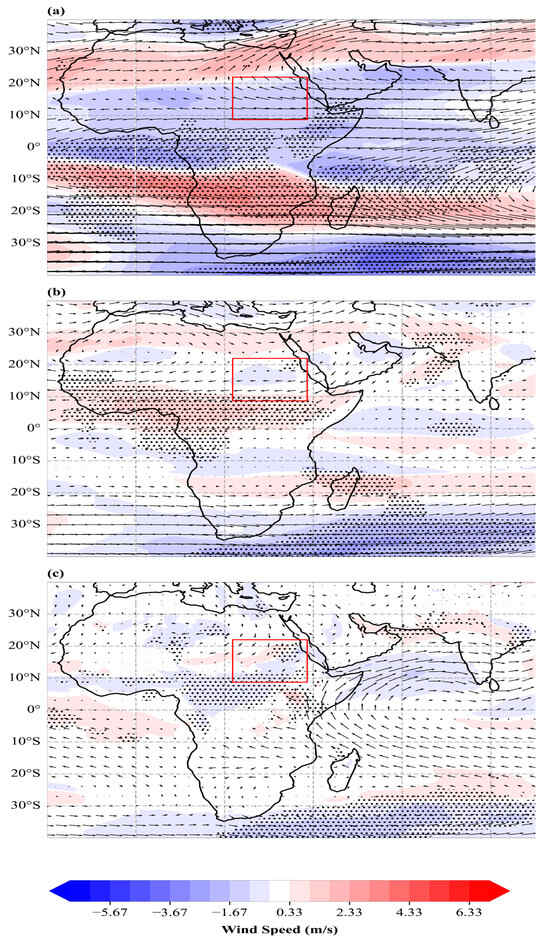
Figure 9.
Illustrates the wind composite anomaly vectors (m/s) for the JJAS system in Africa from 1993 to 2022. Measurements were taken during the dry years at different altitudes. At 200 hPa (a), 500 hPa (b) and 850 hPa. (c). Sudan region is indicated by the red. (The correlation is statistically significant at the 95% confidence level, shown as black dots.)
(b) Pressure System
The CA of the pressure systems driving the rainfall in SDN is illustrated in (Figure 10). Figure 10b shows the pressure systems during dry years (1993, 2002, 2004, 2008, 2009, and 2015) and Figure 10c shows the climatology subtracted from the same dry years (dry–clim). The Southern Indian Ocean (SIO) and Southern Atlantic Ocean (SAO) both have high-pressure (HP) zones that reach SDN, as shown in this figure. In contrast, the East Mediterranean Sea (EMS), North Sahara, and the majority of northern SDN are experiencing low pressure (LP). These pressure systems (Figure 10c) depict the variation in dry years. Overall, in pressure climatology, it appears that subtropical high pressures (SHP) are dominant and have higher values, for example, Azores over the Atlantic Ocean (AO) in the Northern Hemisphere (NH), Muscarine and Sant Helena in the Southern Hemisphere (SH). However, northeastern subtropical anticyclone, i.e., the Cyberia and Arabian Peninsulas, showed negative anomalies in dry years rather than the climatology (Figure 10b). Although the southern SHP and over the equatorial Indian Ocean pole show more positive anomalies than the climatology, this can support the advance of the ITCZ more northward (Figure 10c), the northern HPs revealed negative anomalies. Notably, the North Atlantic Ocean (NAO) and Northwest Pacific showed positive anomalies (Figure 10c), which may indicate that high air pressures had a greater impact on precipitation compared to the LPs in the Atlantic, especially in SDN. In addition, North Sahara, the EMS, and the majority of northern SDN all experienced LP. However, the SIO and SAO both contribute to HP that reaches SDN [33]. The results showed that stronger and weaker combinations of SHP in the north/southern hemisphere affected the movement of the ITCZ over SDN. Though, the Red Sea Hills support the formation of permanent low pressure, which is the primary weather feature in SDN’s eastern departments.
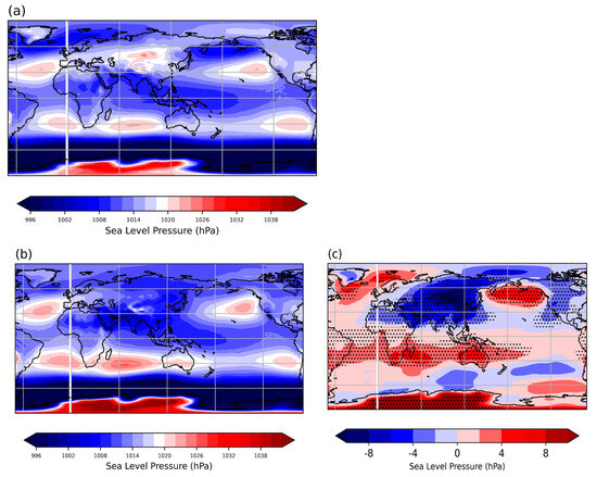
Figure 10.
Mean Sea level pressure during 1993–2022, (a) climatology, (b) dry years, and (c) composite anomaly analysis (dry years—climatology). The correlation is statistically significant at the 95% confidence level, shown as black dots.
4. Conclusions
In summary, the current study intended to provide critical insights into the complex interactions between the Indo-Pacific teleconnections and drought events in SDN for the period from 1993 to 2022. The major outcomes of this investigation can be summarized as follows:
- The SPI during these 30 years highlighted a persistent challenge for Sudan, with frequent and prolonged drought conditions. Specifically, 2002, 2004, 2008, and 2009 were notable drought occurrences. In particular, 2004 is an exceptionally dry year, indicating extreme drought conditions across the region.
- The analysis of the anomaly from mean precipitation in SDN during the selected years (1993, 2002, 2004, 2008, 2009, and 2015) provided insights into drought patterns and their spatial effects. This reveals that the northern regions of SDN, including KH, AJ, and North and South Darfur (western region), consistently experienced drought with varying degrees and extent of impact.
- The Sequential Mann–Kendall and Mann–Kendall trend tests revealed a clear trend of increasing rainfall levels for both JJAS (June, July, August, and September) and annual rainfall after 2016. Before 2016, the rainfall revealed a decreasing trend. The increase in annual precipitation after 2016 was more pronounced than the increase in JJAS rainfall, indicating a potential change in the climate and precipitation dynamics in the region.
- The EOF analysis revealed spatial patterns of rainfall variations in the investigated region. The first EOF mode (42.2%) is the most influential in determining wet and dry conditions during the JJAS season.
- The association with Indo-Pacific Ocean temperatures indicated a strong positive correlation between ENSO, suggesting that negative El Niño Southern Oscillation (ENSO) events may have contributed to the observed dry conditions. Furthermore, a weak positive influence of IOD on JJAS precipitation was observed, as was the first EOF mode in Sudan, which had a significant impact on precipitation amount.
- Composite analysis: (a) The wind circulation patterns, particularly the TEJ, AEJ, SJ and WAM, exert a significant influence on the rainfall patterns across Sudan. The most important of these are the strength and interaction of TEJ and AEJ, which have the strongest correlation with precipitation variability. Additional research is essential to fully understand the effect of wind circulation patterns on precipitation in SDN. (b) The analysis of the pressure systems highlights the significant influence of subtropical high-pressure fluctuations in both hemispheres on the flow of the ITCZ over SDN. It is noteworthy that significant changes in the location and intensity of these high-pressure systems, coupled with the effects of oceanic high- and low-pressure systems, have a direct and measurable impact on precipitation patterns in the region.
Our study is a valuable contribution to the field as it provides timely and relevant information on drought management strategies in SDN. This study does not cover all potential atmospheric drivers, such as: the Madden-Julian Oscillation (MJO), which has not been concluded in this paper and is responsible for the interaction between IOD and ENSO. Despite the limitations, this study has important implications and is a promising advance in our understanding of droughts. Further research is necessary to explore the specific mechanisms driving these interactions, such as MJO, and to develop tailored schemes for mitigating the effects of drought events.
Author Contributions
A.H.A.M., conceptualization, methodology, formal analysis, writing—original draft preparation; X.Z., funding acquisition, recourses, supervision, formal analysis, and investigation; M.A.A.A., methodology, formal analysis, and investigation; all authors participated in writing—review and editing this manuscript. All authors have read and agreed to the published version of the manuscript.
Funding
This work is the Qinglan Project.
Institutional Review Board Statement
Not applicable.
Informed Consent Statement
Not applicable.
Data Availability Statement
The datasets and material used in this study are available from the corresponding author on reasonable request.
Acknowledgments
This study was facilitated by the Nanjing University of Information Science and Technology (NUIST). So, we sincerely acknowledge the NUIST and MOFCOM scholarship. The authors would like to thank all data centers for making their products freely available.
Conflicts of Interest
The authors declare no conflict of interest.
References
- Kallis, G. Droughts. Annu. Rev. Environ. Resour. 2008, 33, 85–118. [Google Scholar] [CrossRef]
- Zhou, H.; Liu, Y.; Liu, Y. An Approach to Tracking Meteorological Drought Migration. Water Resour. Res. 2019, 55, 3266–3284. [Google Scholar] [CrossRef]
- Zhao, R.; Yang, S.; Sun, H.; Zhou, L.; Li, M.; Xing, L.; Tian, R. Extremeness Comparison of Regional Drought Events in Yunnan Province, Southwest China: Based on Different Drought Characteristics and Joint Return Periods. Atmosphere 2023, 14, 1153. [Google Scholar] [CrossRef]
- Su, B.; Huang, J.; Fischer, T.; Wang, Y.; Kundzewicz, Z.W.; Zhai, J.; Sun, H.; Wang, A.; Zeng, X.; Wang, G.; et al. Drought losses in China might double between the 1.5 °C and 2.0 °C warming. Proc. Natl. Acad. Sci. USA 2018, 115, 10600–10605. [Google Scholar] [CrossRef]
- Hao, Z.; Singh, V.P.; Xia, Y. Seasonal Drought Prediction: Advances, Challenges, and Future Prospects. Rev. Geophys. 2018, 56, 108–141. [Google Scholar] [CrossRef]
- FAO. The Impact of Disasters and Crises on Agriculture and Food Security: 2021; FAO: Rome, Italy, 2021. [Google Scholar] [CrossRef]
- Wang, F.; Lai, H.; Li, Y.; Feng, K.; Zhang, Z.; Tian, Q.; Zhu, X.; Yang, H. Dynamic variation of meteorological drought and its relationships with agricultural drought across China. Agric. Water Manag. 2022, 261, 107301. [Google Scholar] [CrossRef]
- Ji, Y.; Fu, J.; Lu, Y.; Liu, B. Three-dimensional-based global drought projection under global warming tendency. Atmos. Res. 2023, 291, 106812. [Google Scholar] [CrossRef]
- Gebremeskel, G.; Tang, Q.; Sun, S.; Huang, Z.; Zhang, X.; Liu, X. Droughts in East Africa: Causes, impacts and resilience. Earth-Sci. Rev. 2019, 193, 146–161. [Google Scholar] [CrossRef]
- Seager, R.; Hoerling, M.; Schubert, S.; Wang, H.; Lyon, B.; Kumar, A.; Nakamura, J.; Henderson, N. Causes of the 2011 to 2014 California drought. J. Clim. 2015, 28, 6997–7024. [Google Scholar] [CrossRef]
- Hoerling, M.; Eischeid, J.; Kumar, A.; Leung, R.; Mariotti, A.; Mo, K.; Schubert, S.; Seager, R. Causes and predictability of the 2012 great plains drought. Bull. Am. Meteorol. Soc. 2014, 95, 269–282. [Google Scholar] [CrossRef]
- Dutra, E.; Magnusson, L.; Wetterhall, F.; Cloke, H.L.; Balsamo, G.; Boussetta, S.; Pappenberger, F. The 2010–2011 drought in the Horn of Africa in ECMWF reanalysis and seasonal forecast products. Int. J. Climatol. 2013, 33, 1720–1729. [Google Scholar] [CrossRef]
- Peterson, T.C.; Heim, R.R., Jr.; Hirsch, R.; Kaiser, D.P.; Brooks, H.; Diffenbaugh, N.S.; Dole, R.M.; Giovannettone, J.P.; Guirguis, K.; Karl, T.R.; et al. Monitoring and Understanding Changes in Heat Waves, Cold Waves, Floods, and Droughts in the United States: State of Knowledge. Bull. Am. Meteorol. Soc. 2013, 94, 821–834. [Google Scholar] [CrossRef]
- Nielsen-Gammon, J.W. The 2011 Texas Drought. Tex. Water J. 2012, 3, 59–95. [Google Scholar] [CrossRef]
- Hussien, A. Analysis of the Drought Impact as an Extreme Climatic Event in Sudan. J. Geosci. Environ. Prot. 2024, 12, 38–47. [Google Scholar] [CrossRef]
- Laki, S.L. Desertification in the Sudan: Causes, effects and policy options. Int. J. Sustain. Dev. World Ecol. 1994, 1, 198–205. [Google Scholar] [CrossRef]
- Mbogo, I. Drought Conditions and Management Strategies in Kenya; Namibia Meteorological Services: Windhoek, Namibia, 2014; pp. 1–9. [Google Scholar]
- Teklu, T.; Von Braum, J.; Zaki, E. Drought and famine relationships in Sudan: Policy implications. Res. Rep.-Int. Food Policy Res. Inst. 1991, 88, 1–3. [Google Scholar] [CrossRef]
- Von Braun, J.; Rose, B. Research report drought and family relationship: Sudan. 1991. Available online: https://www.researchgate.net/publication/5057065_Drought_and_Famine_Relationships_in_Sudan_Policy_Implications (accessed on 2 October 2024).
- Wilhite, D.A. Managing drought risk in a changing climate. Clim. Res. 2016, 70, 99–102. [Google Scholar] [CrossRef]
- Li, T.; Lv, A.; Zhang, W.; Liu, Y. Spatiotemporal Characteristics of Watershed Warming and Wetting: The Response to Atmospheric Circulation in Arid Areas of Northwest China. Atmosphere 2023, 14, 151. [Google Scholar] [CrossRef]
- Yin, H.; Wu, Z.; Fowler, H.J.; Blenkinsop, S.; He, H.; Li, Y. The Combined Impacts of ENSO and IOD on Global Seasonal Droughts. Atmosphere 2022, 13, 1673. [Google Scholar] [CrossRef]
- Andreadis, K.M.; Clark, E.A.; Wood, A.W.; Hamlet, A.F.; Lettenmaier, D.P. Twentieth-century drought in the conterminous United States. J. Hydrometeorol. 2005, 6, 985–1001. [Google Scholar] [CrossRef]
- Liang, X.S. The Liang-Kleeman information flow: Theory and applications. Entropy 2013, 15, 327–360. [Google Scholar] [CrossRef]
- Schubert, S.D.; Stewart, R.E.; Wang, H.; Barlow, M.; Berbery, E.H.; Cai, W.; Hoerling, M.P.; Kanikicharla, K.K.; Koster, R.D.; Lyon, B.; et al. Global meteorological drought: A synthesis of current understanding with a focus on SST drivers of precipitation deficits. J. Clim. 2016, 29, 3989–4019. [Google Scholar] [CrossRef]
- IMasih; Maskey, S.; Mussá, F.E.F.; Trambauer, P. A review of droughts on the African continent: A geospatial and long-term perspective. Hydrol. Earth Syst. Sci. 2014, 18, 3635–3649. [Google Scholar] [CrossRef]
- Haile, G.G.; Tang, Q.; Leng, G.; Jia, G.; Wang, J.; Cai, D.; Sun, S.; Baniya, B.; Zhang, Q. Long-term spatiotemporal variation of drought patterns over the Greater Horn of Africa. Sci. Total Environ. 2020, 704, 135299. [Google Scholar] [CrossRef] [PubMed]
- Kalisa, W.; Zhang, J.; Igbawua, T.; Ujoh, F.; Ebohon, O.J.; Namugize, J.N.; Yao, F. Spatio-temporal analysis of drought and return periods over the East African region using Standardized Precipitation Index from 1920 to 2016. Agric. Water Manag. 2020, 237, 106195. [Google Scholar] [CrossRef]
- Doi, T.; Behera, S.K.; Yamagata, T. On the Predictability of the Extreme Drought in East Africa during the Short Rains Season. Geophys. Res. Lett. 2022, 49, e2022GL100905. [Google Scholar] [CrossRef]
- Funk, C.; Harrison, L.; Shukla, S.; Pomposi, C.; Galu, G.; Korecha, D.; Husak, G.; Magadzire, T.; Davenport, F.; Hillbruner, C.; et al. Examining the role of unusually warm Indo-Pacific sea-surface temperatures in recent African droughts. Q. J. R. Meteorol. Soc. 2018, 144, 360–383. [Google Scholar] [CrossRef]
- Mahmoud, S.H.; Gan, T.Y.; Allan, R.P.; Li, J.; Funk, C. Worsening drought of Nile basin under shift in atmospheric circulation, stronger ENSO and Indian Ocean dipole. Sci. Rep. 2022, 12, 8049. [Google Scholar] [CrossRef]
- Osman, Y.Z.; Shamseldin, A.Y. Qualitative rainfall prediction models for central and southern Sudan using El Nino-southern oscillation and Indian Ocean sea surface temperature indices. Int. J. Climatol. 2002, 22, 1861–1878. [Google Scholar] [CrossRef]
- Alriah, M.A.A.; Bi, S.; Shahid, S.; Nkunzimana, A.; Ayugi, B.; Ali, A.; Bilal, M.; Teshome, A.; Sarfo, I.; Elameen, A.M. Summer monsoon rainfall variations and its association with atmospheric circulations over Sudan. J. Atmos. Sol.-Terr. Phys. 2021, 225, 105751. [Google Scholar] [CrossRef]
- Elramlawi, H.R.; Mohammed, H.I.; Elamin, A.W.; Abdallah, O.A.; Taha, A.A.A.M. Adaptation of Sorghum (Sorghum bicolor L. Moench) Crop Yield to Climate Change in Eastern Dryland of Sudan. In Handbook of Climate Change Resilience; Filho, W.L., Ed.; Springer International Publishing: Cham, Switzerland, 2020; pp. 2549–2573. [Google Scholar] [CrossRef]
- Alriah, M.A.A.; Bi, S.; Nkunzimana, A.; Elameen, A.M.; Sarfo, I.; Ayugi, B. Multiple gridded-based precipitation products’ performance in Sudan’s different topographical features and the influence of the Atlantic Multidecadal Oscillation on rainfall variability in recent decades. Int. J. Climatol. 2022, 42, 9539–9566. [Google Scholar] [CrossRef]
- Philip, S.; Kew, S.F.; van Oldenborgh, G.J.; Otto, F.; O’keefe, S.; Haustein, K.; King, A.; Zegeye, A.; Eshetu, Z.; Hailemariam, K.; et al. Attribution analysis of the Ethiopian drought of 2015. J. Clim. 2018, 31, 2465–2486. [Google Scholar] [CrossRef]
- de Waal, A. Peace and the security sector in Sudan, 2002–2011. Afr. Secur. Rev. 2017, 26, 180–198. [Google Scholar] [CrossRef]
- Santos, J.d.S.; de Oliveira-Júnior, J.F.; Costa, M.d.S.; Cardoso, K.R.A.; Shah, M.; Shahzad, R.; da Silva, L.F.F.F.; Romão, W.M.d.O.; Singh, S.K.; Mendes, D.; et al. Effects of extreme phases of El Niño–Southern Oscillation on rainfall extremes in Alagoas, Brazil. Int. J. Climatol. 2023, 43, 7700–7721. [Google Scholar] [CrossRef]
- Chapman, B.; Rosemond, K. Seasonal climate summary for the southern hemisphere (autumn 2018): A weak La Niña fades, the austral autumn remains warmer and drier. J. South. Hemisph. Earth Syst. Sci. 2020, 70, 328–352. [Google Scholar] [CrossRef]
- Mckee, T.B.; Doesken, N.J.; Kleist, J.R. The Relationship of Drought Frequency and Duration to Time Scales. In Proceedings of the Eighth Conference on Applied Climatology, Anaheim, CA, USA, 17–22 January 1993; Available online: https://api.semanticscholar.org/CorpusID:129950974 (accessed on 15 March 2022).
- Edwards, D.C.; McKee, T.B. Thesis Characteristics of 20th Century Drought in the United States at Multiple Time Scales; Department of Atmospheric Science, Colorado State University: Fort Collins, CO, USA, 1997; Volume 298, p. 155. [Google Scholar]
- Zhang, Z.; Xu, C.Y.; Yong, B.; Hu, J.; Sun, Z. Understanding the changing characteristics of droughts in Sudan and the corresponding components of the hydrologic cycle. J. Hydrometeorol. 2012, 13, 1520–1535. [Google Scholar] [CrossRef]
- Awange, J.L.; Khandu; Schumacher, M.; Forootan, E.; Heck, B. Exploring hydro-meteorological drought patterns over the Greater Horn of Africa (1979-2014) using remote sensing and reanalysis products. Adv. Water Resour. 2016, 94, 45–59. [Google Scholar] [CrossRef]
- Guenang, G.M.; Kamga, F.M. Computation of the standardized precipitation index (SPI) and its use to assess drought occurrences in Cameroon over recent decades. J. Appl. Meteorol. Climatol. 2014, 53, 2310–2324. [Google Scholar] [CrossRef]
- Ugwu, E.B.I.; Ugbor, D.O.; Agbo, J.U.; Alfa, A. Analyzing rainfall trend and drought occurences in Sudan Savanna of Nigeria. Sci. Afr. 2023, 20, e01670. [Google Scholar] [CrossRef]
- Lloyd-Hughes, B.; Saunders, M.A. A drought climatology for Europe. Int. J. Climatol. 2002, 22, 1571–1592. [Google Scholar] [CrossRef]
- Svoboda; Hayes, M.; Wood, D. Standradized Precipitation Index User Guide; WMO: Geneva, Switzerland, 2012. [Google Scholar]
- Wilks, D.S. Preface. In Statistical Methods in the Atmospheric Sciences; International Geophysics Series; Academic Press: Cambridge, MA, USA, 2006; Volume 59. [Google Scholar] [CrossRef]
- Nicholson, S.E. Climate and climatic variability of rainfall over eastern Africa. Rev. Geophys. 2017, 55, 590–635. [Google Scholar] [CrossRef]
- dar, J.; dar, A.Q. Spatio-temporal variability of meteorological drought over India with footprints on agricultural production. Environ. Sci. Pollut. Res. 2021, 28, 55796–55809. [Google Scholar] [CrossRef] [PubMed]
- Rayner, N.a. A Manual for EOF and SVD. J. Geophys. Res. 1997, 108, 4407. [Google Scholar] [CrossRef]
- Oktaviani, F.; Miftahuddin; Setiawan, I. Cross-correlation Analysis between Sea Surface Temperature Anomalies and Several Climate Elements in the Indian Ocean. Parameter J. Stat. 2021, 1, 13–20. [Google Scholar] [CrossRef]
- Mclean, L.D.; Guilford, J.P.; Fruchter, B. Fundamental Statistics in Psychology and Education. 1943. Available online: https://api.semanticscholar.org/CorpusID:145224068 (accessed on 2 October 2024).
- Bayable, G.; Gashaw, T. Spatiotemporal variability of agricultural drought and its association with climatic variables in the Upper Awash Basin, Ethiopia. SN Appl. Sci. 2021, 3, 465. [Google Scholar] [CrossRef]
- Colman, A.W.; Graham, R.J.; Davey, M.K. Direct and indirect seasonal rainfall forecasts for East Africa using global dynamical models. Int. J. Climatol. 2020, 40, 1132–1148. [Google Scholar] [CrossRef]
- Kipkogei, O.; Mwanthi, A.M.; Mwesigwa, J.B.; Atheru, Z.K.K.; Wanzala, M.A.; Artan, G. Improved seasonal prediction of rainfall over East Africa for application in agriculture: Statistical downscaling of CFSv2 and GFDL-FLOR. J. Appl. Meteorol. Climatol. 2017, 56, 3229–3243. [Google Scholar] [CrossRef]
- Ogwang, B.A.; Ongoma, V.; Xing, L.; Ogou, F.K. Influence of mascarene high and Indian Ocean dipole on East African extreme weather events. Geogr. Pannonica 2015, 19, 64–72. [Google Scholar] [CrossRef]
- Omondi, P.; Ogallo, L.A.; Anyah, R.; Muthama, J.M.; Ininda, J. Linkages between global sea surface temperatures and decadal rainfall variability over Eastern Africa region. Int. J. Climatol. 2013, 33, 2082–2104. [Google Scholar] [CrossRef]
- Welhouse, L.J.; Lazzara, M.A.; Keller, L.M.; Tripoli, G.J.; Hitchman, M.H. Composite analysis of the effects of ENSO events on Antarctica. J. Clim. 2016, 29, 1797–1808. [Google Scholar] [CrossRef]
- Nkunzimana, A.; Shuoben, B.; Guojie, W.; Alriah, M.A.A.; Sarfo, I.; Zhihui, X.; Vuguziga, F.; Ayugi, B.O. Assessment of drought events, their trend and teleconnection factors over Burundi, East Africa. Theor. Appl. Climatol. 2021, 145, 1293–1316. [Google Scholar] [CrossRef]
- Partal, T.; Kahya, E. Trend analysis in Turkish precipitation data. Hydrol. Process. 2006, 20, 2011–2026. [Google Scholar] [CrossRef]
- Ongoma, V.; Chen, H. Temporal and spatial variability of temperature and precipitation over East Africa from 1951 to 2010. Meteorol. Atmos. Phys. 2017, 129, 131–144. [Google Scholar] [CrossRef]
- Tan, C.; Yang, J.; Li, M. Temporal-spatial variation of drought indicated by SPI and SPEI in Ningxia Hui Autonomous Region, China. Atmosphere 2015, 6, 1399–1421. [Google Scholar] [CrossRef]
- Esit, M.; Yuce, M. Comprehensive evaluation of trend analysis of extreme drought events in the Ceyhan River Basin, Turkey. Meteorol. Hydrol. Water Manag. 2022, 11, 22–43. [Google Scholar] [CrossRef]
- Liu, C.; Yang, C.; Yang, Q.; Wang, J. Spatiotemporal drought analysis by the standardized precipitation index (SPI) and standardized precipitation evapotranspiration index (SPEI) in Sichuan Province, China. Sci. Rep. 2021, 11, 1280. [Google Scholar] [CrossRef]
- Jain, S.K.; Kumar, V. Trend analysis of rainfall and temperature data for India. Curr. Sci. 2012, 102, 37–49. [Google Scholar]
- Mohmmed, A.; Zhang, K.; Kabenge, M.; Keesstra, S.; Cerdà, A.; Reuben, M.; Elbashier, M.M.; Dalson, T.; Ali, A.A. Analysis of drought and vulnerability in the North Darfur region of Sudan. Land Degrad. Dev. 2018, 29, 4424–4438. [Google Scholar] [CrossRef]
- Alriah, M.A.A.; Bi, S.; Nkunzimana, A.; Elameen, A.M.; Sarfo, I.; Ayugi, B. Assessment of observed changes in drought characteristics and recent vegetation dynamics over arid and semiarid areas in Sudan. Theor. Appl. Climatol. 2024, 155, 3541–3561. [Google Scholar] [CrossRef]
- Ngarukiyimana, J.P.; Fu, Y.; Yang, Y.; Ogwang, B.A.; Ongoma, V.; Ntwali, D. Dominant atmospheric circulation patterns associated with abnormal rainfall events over Rwanda, East Africa. Int. J. Climatol. 2018, 38, 187–202. [Google Scholar] [CrossRef]
- Ongoma, V.; Chen, H.; Omony, G.W. Variability of extreme weather events over the equatorial East Africa, a case study of rainfall in Kenya and Uganda. Theor. Appl. Climatol. 2018, 131, 295–308. [Google Scholar] [CrossRef]
- Sian, K.T.C.L.K.; Dosio, A.; Ayugi, B.O.; Hagan, D.F.T.; Kebacho, L.L.; Ongoma, V. Dominant modes of precipitation over Africa, and their associated atmospheric circulations from observations. Int. J. Climatol. 2023, 43, 4603–4618. [Google Scholar] [CrossRef]
- Ndomeni, C.W.; Cattani, E.; Merino, A.; Levizzani, V. An observational study of the variability of East African rainfall with respect to sea surface temperature and soil moisture. Q. J. R. Meteorol. Soc. 2018, 144, 384–404. [Google Scholar] [CrossRef]
- Endris, H.S.; Lennard, C.; Hewitson, B.; Dosio, A.; Nikulin, G.; Artan, G.A. Future changes in rainfall associated with ENSO, IOD and changes in the mean state over Eastern Africa. Clim. Dyn. 2019, 52, 2029–2053. [Google Scholar] [CrossRef]
- El Gamri, T.; Saeed, A.B.; Abdalla, A. Rainfall of the Sudan: Characteristics and Prediction. J. Fac. Arts Univ. Khartoum 2021, 27, 17–35. [Google Scholar] [CrossRef]
- Kebacho, L. Large-scale circulations associated with recent interannual variability of the short rains over East Africa. Meteorol. Atmos. Phys. 2022, 134, 10. [Google Scholar] [CrossRef]
- Kebacho, L.L.; Sarfo, I. Why Eastern Africa was not dry during the 2020 short rainy season despite La Niña and a negative Indian Ocean Dipole: Interplay between the Madden-Julian Oscillation and La Niña in modulating short rain. Theor. Appl. Climatol. 2023, 153, 1191–1201. [Google Scholar] [CrossRef]
- Hulme, M.; Tosdevin, N. The Tropical easterly Jet and Sudan rainfall: A review. Theor. Appl. Climatol. 1989, 39, 179–187. [Google Scholar] [CrossRef]
- Mishra, S.K.; Tandon, M.K. A combined barotropic-baroclinic instability study of the upper tropospheric tropical easterly jet. J. Atmos. Sci. 1983, 40, 2708–2723. [Google Scholar] [CrossRef][Green Version]
- Druyan, L.M.; Koster, R.D. Sources of Sahel Precipitation for Simulated Drought and Rainy Seasons. J. Clim. 1989, 2, 1438–1446. [Google Scholar] [CrossRef]
- Lélé, M.I.; Lamb, P.J. Variability of the Intertropical Front (ITF) and rainfall over the West African Sudan-Sahel zone. J. Clim. 2010, 23, 3984–4004. [Google Scholar] [CrossRef]
- Agustí-Panareda, A.; Beljaars, A.; Cardinali, C.; Genkova, I.; Thorncroft, C. Impacts of assimilating AMMA soundings on ECMWF analyses and forecasts. Weather Forecast. 2010, 25, 1142–1160. [Google Scholar] [CrossRef]
- Vizy, E.K.; Cook, K.H. Connections between the summer east African and Indian rainfall regimes. J. Geophys. Res. Atmos. 2003, 108, 4510. [Google Scholar] [CrossRef]


Disclaimer/Publisher’s Note: The statements, opinions and data contained in all publications are solely those of the individual author(s) and contributor(s) and not of MDPI and/or the editor(s). MDPI and/or the editor(s) disclaim responsibility for any injury to people or property resulting from any ideas, methods, instructions or products referred to in the content. |
© 2024 by the authors. Licensee MDPI, Basel, Switzerland. This article is an open access article distributed under the terms and conditions of the Creative Commons Attribution (CC BY) license (https://creativecommons.org/licenses/by/4.0/).