Review

Current Situation and Prospect of Geospatial AI in Air Pollution Prediction

1
School of Automation, University of Electronic Science and Technology of China, Chengdu 610054, China
2
Department of Computer Science and Engineering, Hanyang University, Ansan 15577, Republic of Korea
3
Department of Geography & Anthropology, Louisiana State University, Baton Rouge, LA 70803, USA
*
Authors to whom correspondence should be addressed.
Atmosphere 2024, 15(12), 1411; https://doi.org/10.3390/atmos15121411
Submission received: 22 October 2024 / Revised: 17 November 2024 / Accepted: 20 November 2024 / Published: 24 November 2024
(This article belongs to the Section Atmospheric Techniques, Instruments, and Modeling)

Abstract

:
Faced with increasingly serious environmental problems, scientists have conducted extensive research, among which the importance of air quality prediction is becoming increasingly prominent. This article briefly reviews the utilization of geographic artificial intelligence (AI) in air pollution. Firstly, this paper conducts a literature metrology analysis on the research of geographical AI used in air pollution. That is, 607 documents are retrieved from the Web of Science (WOS) using appropriate keywords, and literature metrology analysis is conducted using Citespace to summarize research hotspots and frontier countries in this field. Among them, China plays a constructive role in the fields of geographic AI and air quality research. The data characteristics of Earth science and the direction of AI utilization in the field of Earth science were proposed. It then quickly expanded to investigate and research air pollution. In addition, based on summarizing the current status of Artificial Neural Network (ANN), Recurrent Neural Network (RNN), and hybrid neural network models in predicting air quality (mainly PM2.5), this article also proposes areas for improvement. Finally, this article proposes prospects for future research in this field. This study aims to summarize the development trends and research hotspots of the utilization of geographic AI in the prediction of air quality, as well as prediction methods, to provide direction for future research.

1. Introduction

Recently, the issue of air pollution has caused great concern in all countries around the world as well as various sectors of society and has become the focus of discussion for many scholars. Air pollution seriously harms physical health and has huge adverse effects on production work. Figure 1 shows the negative effect of haze on the human body. Haze can cause various degrees of injury to the lungs [1], eyes [2,3], skin and hair [4,5,6], liver [7], bones [8,9,10], mind [11,12,13], intestines [14,15], reproductive systems [16,17], and hearts [18,19]. Therefore, it is urgent to address the issue of air pollution to ensure the sustainable development of society and maintain a healthy standard of living for all. To help people better plan their lives and work, reduce the health risks posed by air pollution, and assist governments and enterprises in formulating more intelligent and rigorous environmental policies and measures to solve air pollution problems, the use of AI technology to predict air quality is a significant prerequisite for achieving this goal [20].
Air quality describes the concentration and composition of pollutants, indicating the degree of air pollution. Goodman, Nigel, and others use air quality to describe the degree of air pollution caused by air fresheners [21]. Lee, Jungsuk, et al. also used air quality to measure the virus content in inpatient wards [22]. Consequently, obtaining air pollution information, implementing preventive measures, and promptly adopting safety precautions are crucial for the reduction in health risks posed by exposure to air pollution [23].
Earth science refers to all the sciences that study the earth, including geology, meteorology, and other derivative sciences. Artificial intelligence, encompassing methodologies such as machine learning (ML) and deep learning (DL), has become notably popular in geosciences due to its capabilities in recognizing complex patterns and processing vast quantities of data. The integration of these computational approaches enables scientists to extract meaningful insights from multi-dimensional datasets and model intricate environmental systems with unprecedented accuracy and efficiency.
In some models and applications, earth science data share some common characteristics, and we summarize in Figure 2:
The following is a detailed description:
  • Rare phenomena, such as earthquakes [24], hurricanes [25], and floods [26], people in these extreme weather or natural disasters very fragile, and it is easy to cause irreparable loss of life and fortune. Therefore, it is essential to predict and evaluate these phenomena.
  • Data fragility. Data sources in earth sciences are usually sensors and earth observation satellites. However, sensor crashes caused by satellite updates, malfunctions, or bad weather can easily lead to data loss [27,28].
  • High dimensions. Many earth science phenomena are not confined to the earth’s surface, just like typhoons [29], volcanism [30], geothermal [31], and geomagnetic phenomena all extend below the surface.
  • It has an obvious space–time structure. First, the occurrence of earth science phenomena such as haze [32], volcanic eruption [33], and earthquake [34] has obvious time and space characteristics. Secondly, due to the great variability of the earth’s vegetation, rock strata, and climate in time and space, the input variables of earth science vary greatly in different locations.
AI tools have a broad spectrum of applications in Earth science. Figure 3 shows the four major applications of artificial intelligence in Earth science.
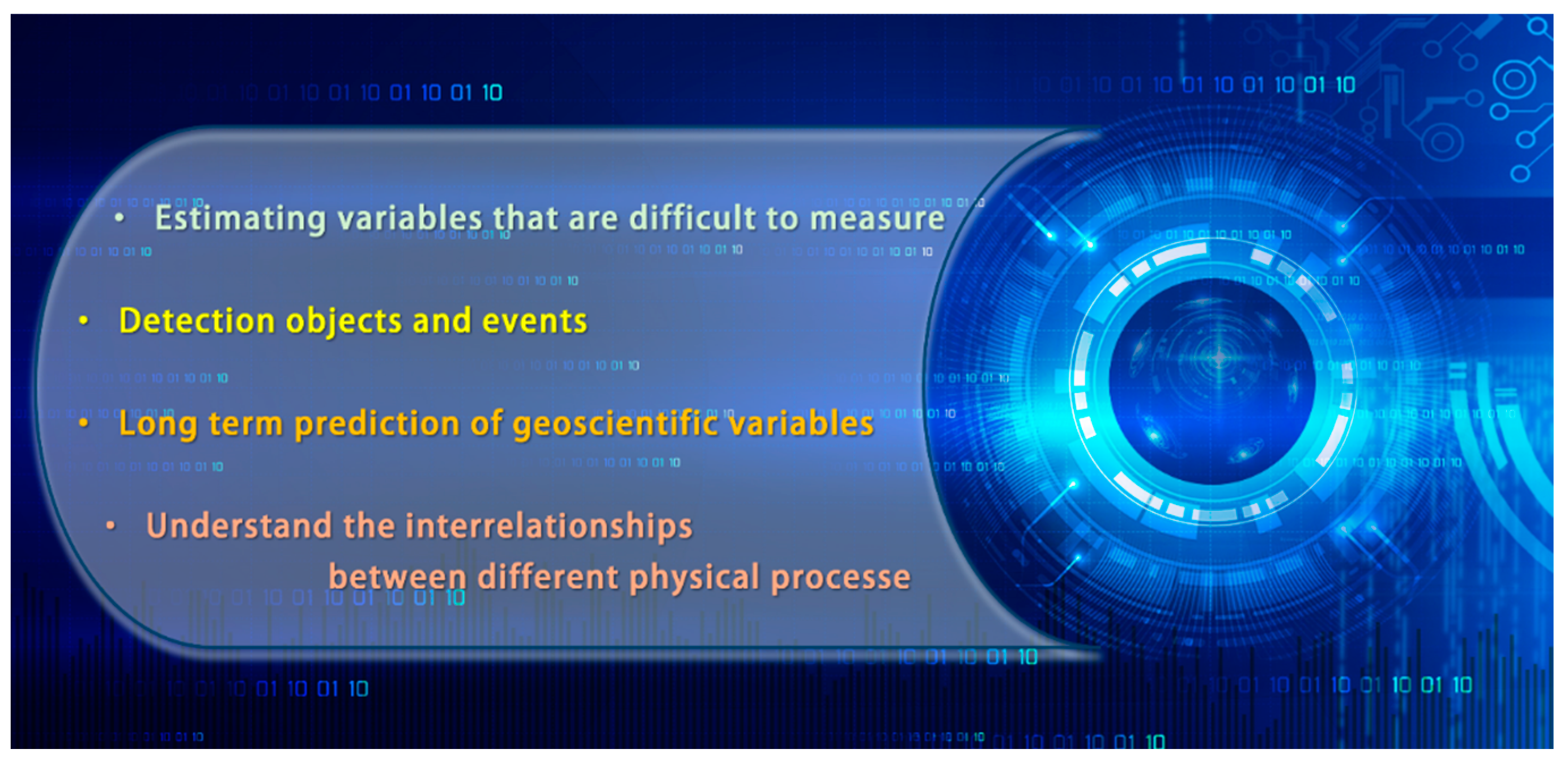
  • Estimating Difficult to Measure Variables: Artificial intelligence can use machine learning techniques to estimate Earth science variables that are difficult to measure. Relying on artificial intelligence algorithms, these previously difficult to measure geoscientific variables become precise.
  • Detection of objects and events: AI tools can detect objects and events in Earth science through technologies such as image recognition and speech recognition. Li et al. [35] developed LOC-FLOW, a seismic detection and location workflow based on deep learning, to construct a high-precision microseismic catalog for the Xiluodu Reservoir area. This AI-generated catalog was then used in combination with conventional seismic array data to perform 3D velocity structure inversion and precise earthquake relocation. This AI-generated catalog containing 6595 earthquakes was integrated with conventional seismic array data to enhance ray coverage and improve the resolution of velocity structure imaging.
  • Long-term prediction of geoscience variables: Artificial intelligence can predict the long-term trends and periodic changes in geoscience variables, such as precipitation, climate change, sea level rise, etc., through techniques such as time series analysis and deep learning. Jin, Weixin et al.’s study guided precipitation prediction based on deep learning models [36].
  • Understand the interrelationships between different physical processes: Artificial intelligence can use techniques such as data mining and model analysis to understand the interrelationships between different physical processes.
Researchers exploring air quality prediction models have shown significant interest in approaches that combine machine learning with deep learning. These methodologies have proven effective in this domain, particularly due to their capacity to handle time series and non-linear data. The research conducted by Pak and colleagues [37] introduced an innovative hybrid model that integrates convolutional neural networks with long short-term memory networks. This advanced framework was specifically designed to generate accurate forecasts of the subsequent day’s mean PM2.5 levels in Beijing’s urban atmosphere. Another significant contribution was made by Duen-ren Liu et al. [38], who introduced an innovative PM2.5 concentration prediction model for air pollution. This model, built on attention mechanisms and LSTM neural networks, was designed to forecast PM2.5 levels for the upcoming 6–24 h. A key finding of their research was the importance of incorporating PM2.5 pollution drift patterns and weather forecast data into the prediction framework.
Recent advances in AI, particularly in machine learning and deep learning, have opened new possibilities for more accurate and reliable air pollution forecasting. These technologies offer powerful tools for processing vast quantities of environmental data and identifying complex patterns that may not be apparent through conventional analysis methods. However, despite the growing body of research in this field, there remains a significant need for a comprehensive understanding of how these technologies are being applied and their effectiveness in air quality prediction.
This study aims to address this gap through three primary objectives:
First, we present a detailed bibliometric analysis using the Web of Science Core Collection, examining 607 publications to identify research trends, influential works, and emerging areas of focus. This analysis offers insights into the temporal evolution of research interests and methodological approaches in the field.
Second, we provide a comprehensive review of AI applications in Earth science, particularly focusing on their application to air quality prediction. This includes examinations of various neural network architectures, from basic Artificial Neural Networks (ANNs) to more sophisticated hybrid models, evaluating their relative strengths and limitations in handling the unique characteristics of environmental data.
Third, we analyze the integration of AI with Internet of Things (IoT) technologies and smart sensors in air quality monitoring and prediction, exploring how these combinations enhance prediction accuracy and spatial coverage. The challenges associated with data collection, including issues of sensor reliability and data quality, are also examined.
The remainder of this paper is organized as follows: Section 2 presents our bibliometric analysis methodology and findings. Section 3 examines the current state and applications of AI in air quality prediction, including a detailed analysis of different modeling approaches. Section 4 discusses current limitations and challenges in the field. Finally, Section 5 concludes with insights into future research directions and potential developments in this rapidly evolving domain.
This systematic review aims to provide researchers, environmental scientists, and policymakers with a comprehensive understanding of the current state of AI applications in air quality prediction while also identifying promising directions for future research and development in this critical field.

2. Bibliometric Analysis

Bibliometrics can be used to quantitatively analyze the structure, characteristics, and connections of a domain. CiteSpace (V6.3.R1, Drexel University, Philadelphia, PA, USA), is a tool for visualizing and analyzing trends and patterns in scientific literature. It helps researchers and scholars identify the most influential articles, authors, and research topics within a specific field. Compared with other tools such as the VOSViewer (V1.6.19, Leiden University, Leiden, Netherlands) and Science of Science (SCI2) Tool (V2.0 Alpha, Indiana University, Bloomington, IN, USA), CiteSpace can better indicate the betweenness centrality of nodes within the network connections and reflect the characteristics of research changes over time. To obtain the latest direction and research hotspot of geographic artificial intelligence on air pollution, we conducted a comprehensive review of the pertinent literature through bibliometric analysis. We chose the Web of Science (WOS) Core Collection as the literature database due to its rich resources and recognized authority and influence in the academic community. The WOS Core Collection covers various fields with rich scholarly resources and over a billion citation records, which provide a solid foundation for our bibliometric analysis. The specific operational process is as follows: Using the WOS Core Collection database. We took “Deep learning” and “air pollution” as the “subject”. The search date was from 1 January 2012 to 31 December 2023, as this time span covers the period of rapid development in geographical AI research related to air pollution. In order to ensure the accuracy of the data and the validity of the analysis, we deleted the repeated search results, ultimately identifying 607 articles in total. The full content of these 607 articles was exported in plain text format to constitute the dataset for this study. Citespace 6.2 R4 was used to conduct analysis from four perspectives: literature development, citation journals and research topics, keyword co-occurrence analysis, and cluster analysis.

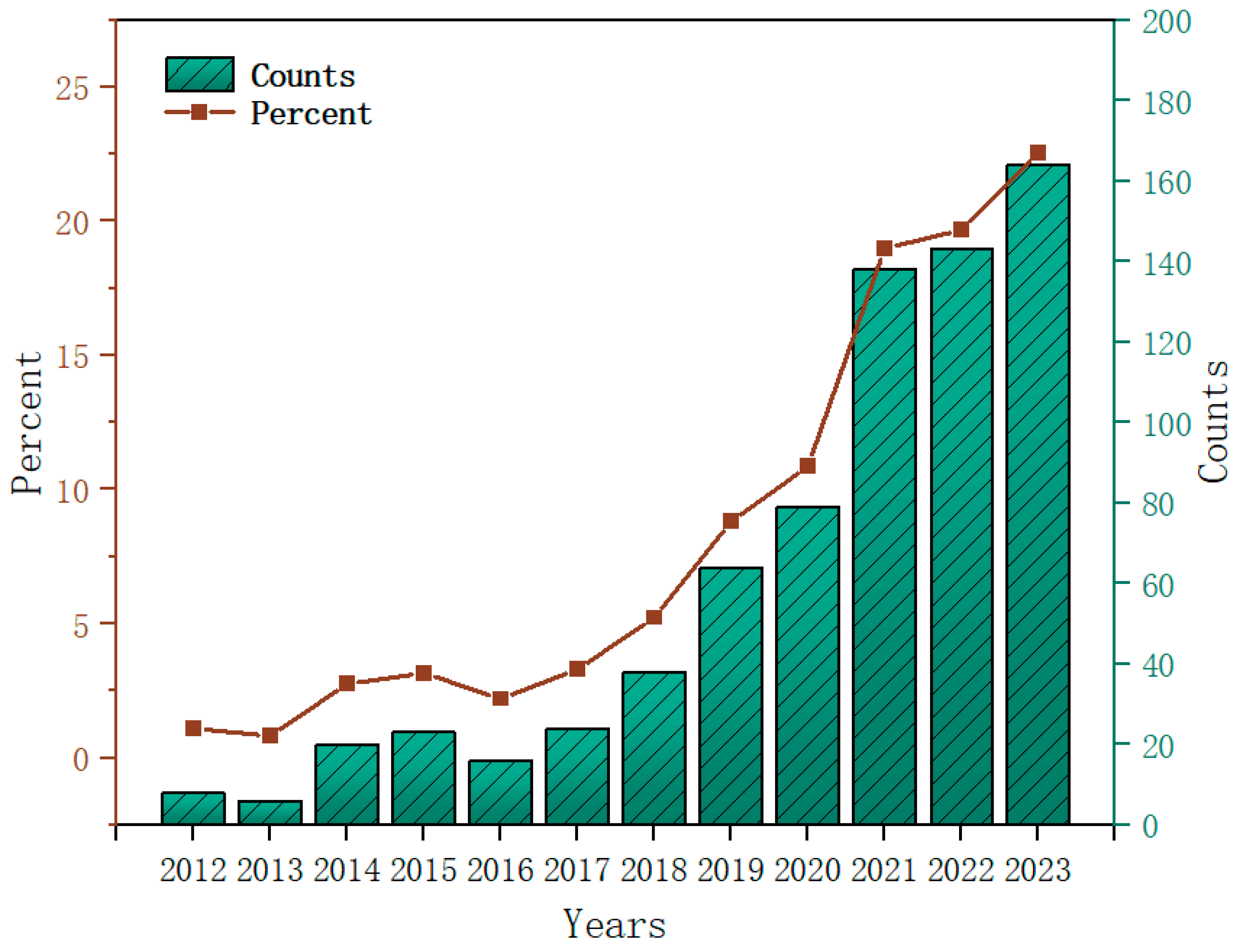
2.1. Literature Development Trend

The number of publications can be a valuable metric for tracking the evolving trends in geographical AI research related to air pollution. Figure 4 shows the annual distribution of papers and their percentage of the total, and overall, research in this discipline continues to show rapid growth. The year 2017 was a key year, with an average of 40 or more publications per year after 2017, indicating widespread academic interest in the issue.

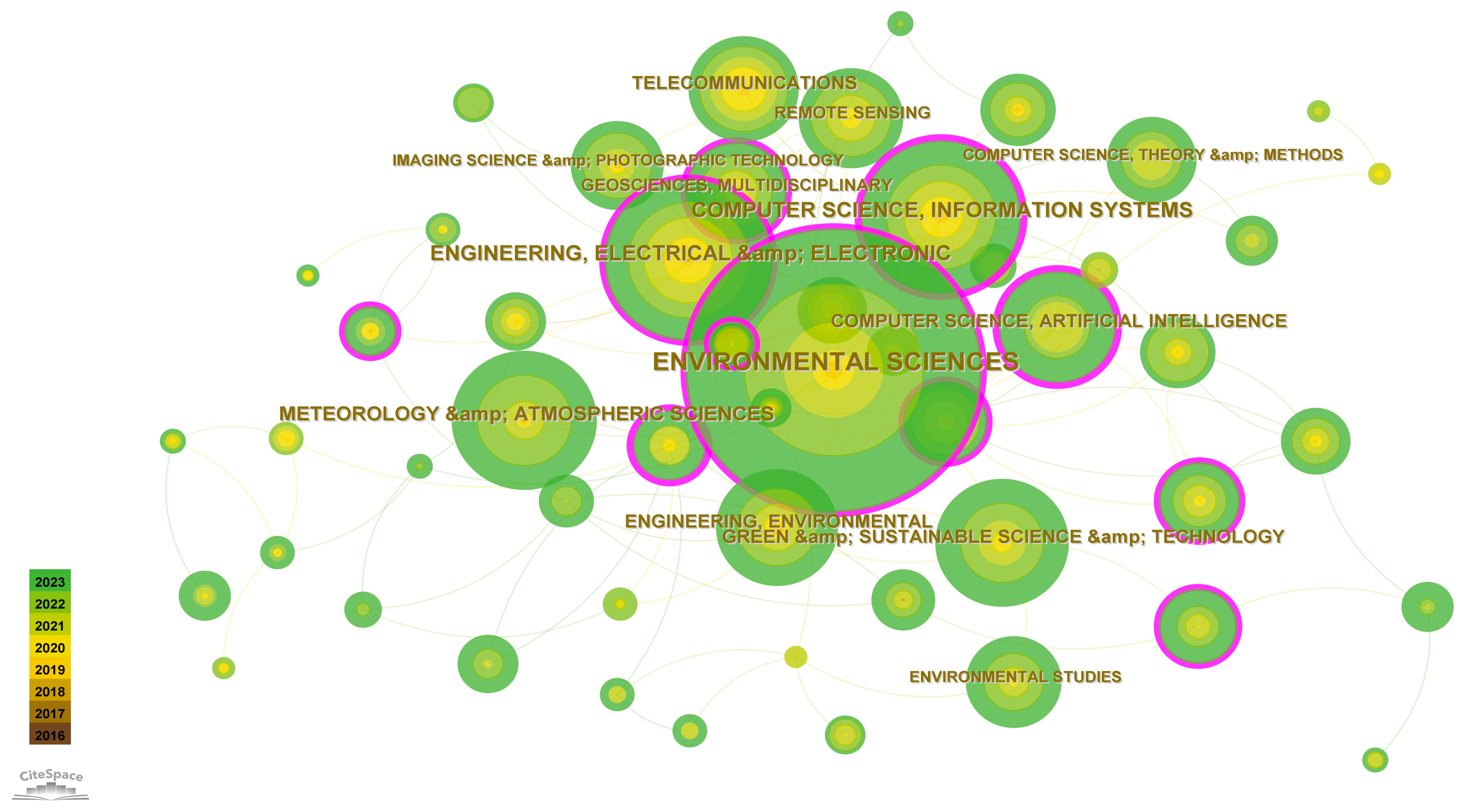
2.2. Cite Journals and Research Topics

‘Atmosphere’, ‘Atmospheric Pollution Research’, and ‘Atmospheric Environment’ are the three most frequently cited journals, published by MDPI, TUNCAP, and Elsevier. Table 1 presents the top 10 journals and their related information.
Then, as shown in Figure 5, we used CitesSpace to plot the research topic contribution network. The size of each node indicates how often the topic appears, and the purple border around it indicates its intermediate centrality, with thicker borders indicating higher intermediate centrality and greater academic significance. Lines connecting nodes represent academic connections between different domains, and thicker lines signify stronger academic connections.
The research area is obviously divided into two directions. One is focused on environmental science, which has important academic links with ecology and engineering. The other direction is rooted in computer science, closely linked with atmospheric science and electronic informatics. Linking these two directions shows that environmental science and computer science are central to the theme of this study.

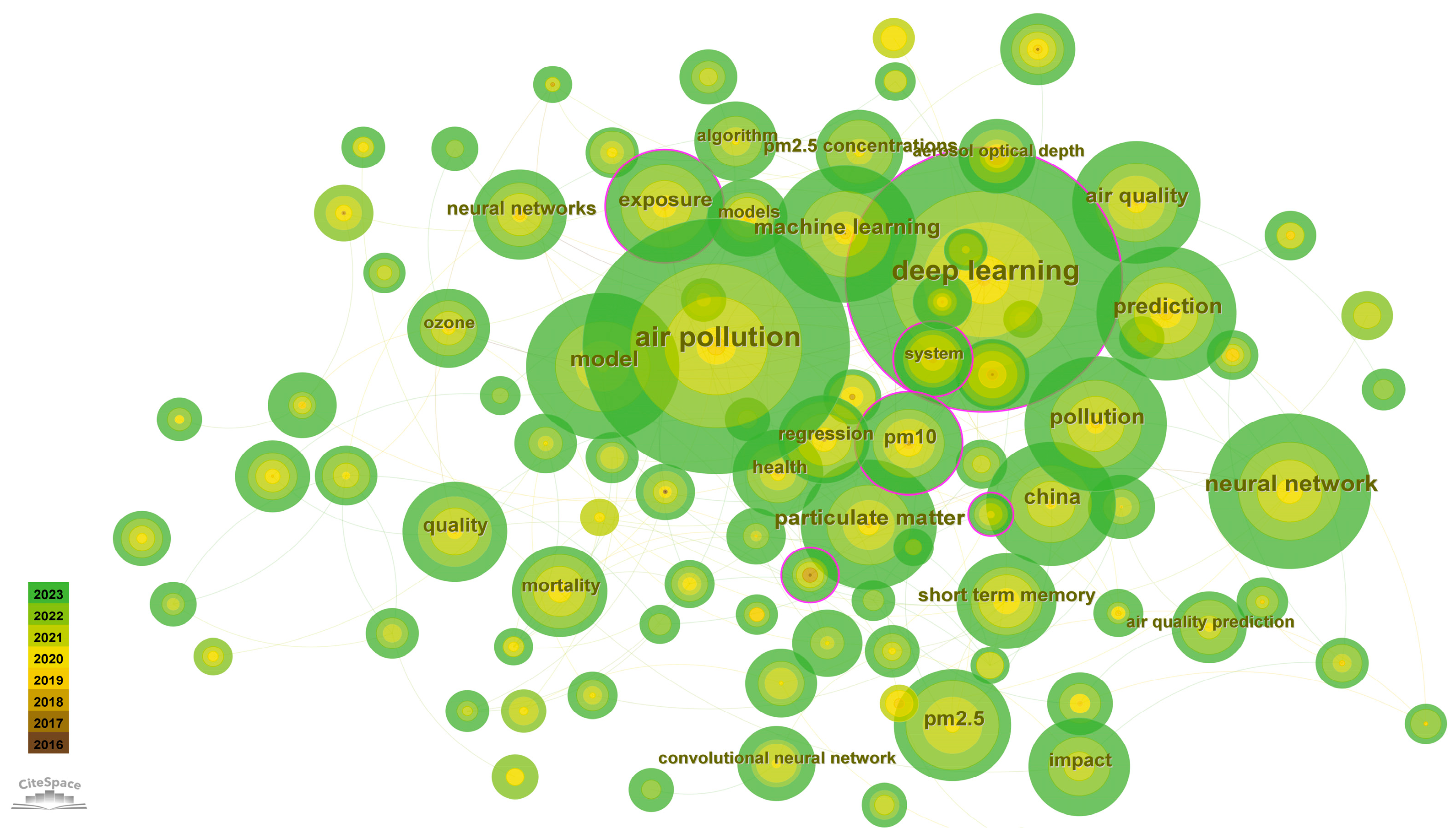
2.3. Keyword Co-Occurrence

A “mutant word” refers to a keyword that has been cited frequently over a specific period, serving as an indicator for emerging research topics. In Table 2, we display some of the “mutant words”, where the last column indicates the time when the “mutant words” appear. The blue line illustrates the timeline, with the red segment of the blue line indicating the period in which the keyword burst. The top five keywords by duration are: Ambient Air (2013–2019), Particulate Air Pollution (2012–2018), Aerosol (2012–2018), Temporal Variation (2014–2018), and Seasonal Variation (2014–2018).
Keyword co-occurrence can effectively highlight focal areas of research in this field, while burst keywords reveal emerging topics. To explore these research trends and cutting-edge issues, we analyzed the distribution of keywords, beginning with the keyword co-occurrence network (Figure 6).
Like Figure 5, nodes in Figure 6 represent keywords, with node size indicating the frequency of articles featuring those keywords in the field of electroluminescence. The connection lines between nodes represent the relationships between keywords. The top ten keywords include air pollution, PM10, particulate matter, deep learning, PM2.5, pollution, prediction, asthma, neural networks, and China. It is observable that PM2.5 and PM10 are the inhalable particles that have received the main attention, and the research direction of scholars is mostly the prediction of inhalable particle concentration based on artificial networks, and China is the main research country.

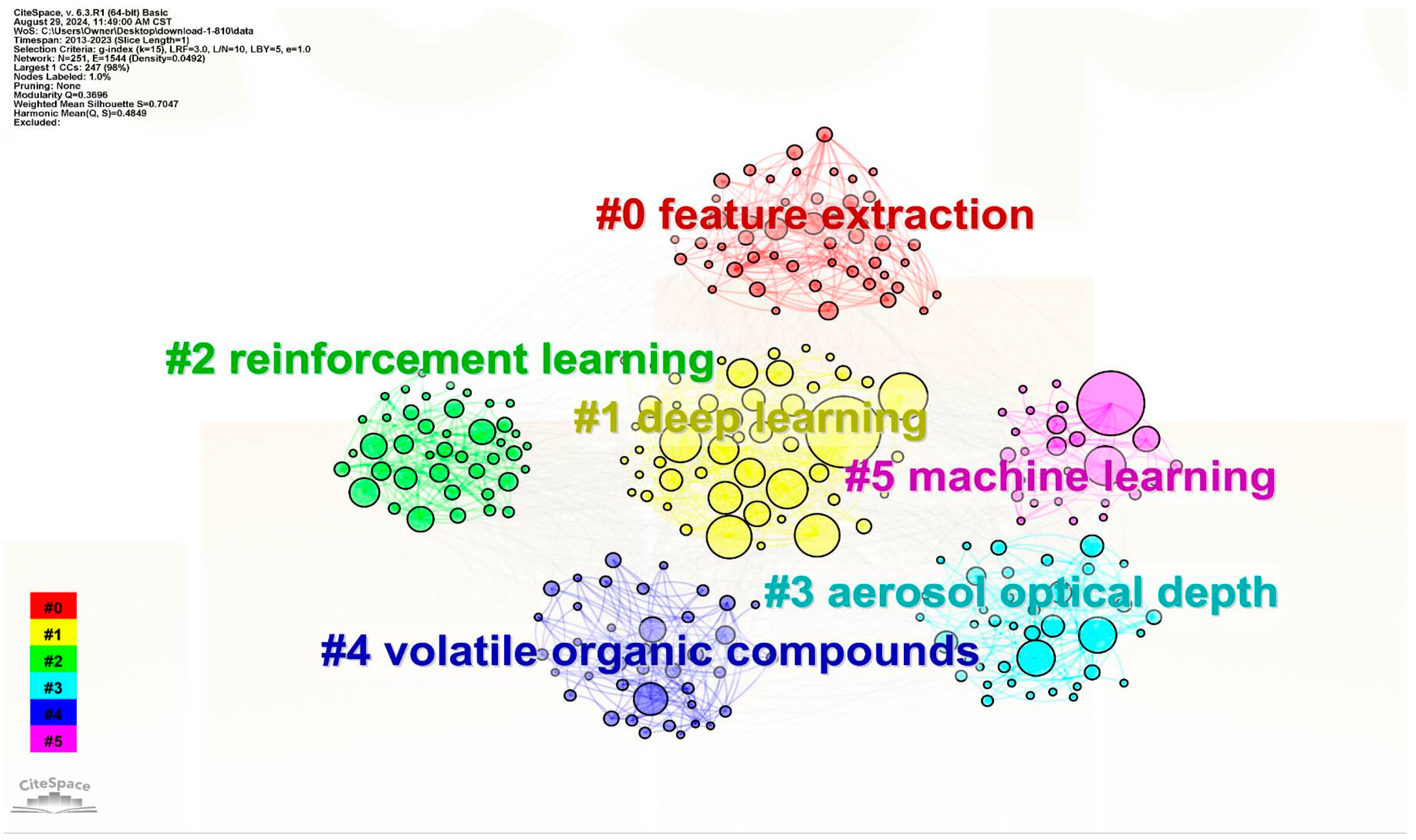
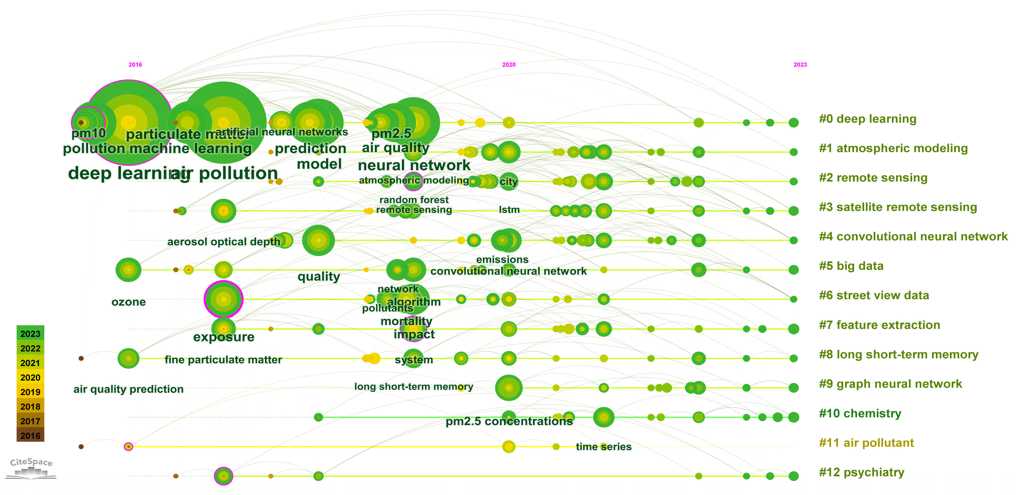
2.4. Cluster Analysis

Under the co-occurrence graph of keywords, keyword clustering and timeline analysis can be performed to group closely related keywords, thereby revealing research hotspots and developing trends in the domain. From 2012 to 2023, all articles in this field were clustered using the logarithmic likelihood method (LLR), where nodes represent different common keywords corresponding to various professional or thematic clusters.
In Figure 7, the clustering modularity Q is 0.3696   ( Q > 0.3 ) , and Weighted Mean Silhouette S is 0.7047   ( S > 0.7 ) , indicating that the clustering is truly effective.
Co-occurrence keywords are divided into five subsets: ‘feature extraction’, ‘deep learning’, ‘reinforcement learning’, ‘aerosol optical depth’, ‘volatile organic compounds’, and ‘machine learning’.
In addition, as Figure 8 has shown, the clustering timeline map illustrates the temporal development of keywords under a certain cluster.
Among them, the period from 2016 to 2018 is the most intensive period of keyword nodes, during which new methods such as deep learning continue to emerge and research output continues to increase. ‘Deep learning’ has been studied by scholars from 2016 to 2023, with a long time span and a large number of publications, which can be used as a long-term research direction. ‘Machine learning’ has a long time span but a small number of published documents.

3. Current Situation and Application

3.1. Air Quality Prediction

Air quality characterizes the levels and makeup of contaminants in the atmosphere, reflecting the extent of atmospheric pollution. In the field of atmospheric monitoring, the primary focus typically centers on the concentration of suspended particulate matter, with particular attention given to PM2.5 and PM10 levels. These classifications refer to particles with aerodynamic diameters not exceeding 2.5 and 10 μm, respectively. The quantification of these airborne particulates is a key metric for assessing the overall quality of ambient air and its potential effects on human health and the environment.
Contaminants in the air can be divided into two main categories according to their physical state: particulate matter in suspension and gaseous compounds. PM2.5, which substantially affects both air clarity and quality, falls under the category of suspended particulate matter. In recent literature, the approaches to predicting PM2.5 concentrations have largely centered around two methodologies.
The first approach involves deterministic frameworks, also referred to as Chemical Transport Models (CTMs), which are analytical tools designed for simulating the spread and chemical evolution of contaminants within the atmosphere [39]. These models integrate various physical and chemical mechanisms, including convection, dispersal, molecular interactions, and settling, to predict atmospheric quality and elucidate the origins, sinks, and movement of pollutants. However, the majority of deterministic models demand extensive computational resources and detailed parametric knowledge yet often yield limited accuracy. Furthermore, prior studies indicate that the dynamic and intricate nature of atmospheric conditions frequently undermines the effectiveness of deterministic models. Consequently, while these models offer valuable insights into pollutant behavior, their practical application remains constrained.
The second approach employs statistical techniques, which aim to overcome certain limitations inherent in deterministic methods. Unlike their deterministic counterparts, statistical approaches do not depend on intricate physical parameters; instead, they forecast pollutant levels by analyzing past records. Given sufficient historical information, statistical techniques can be applied effectively. Nevertheless, these models have their own shortcomings, primarily due to their frequent reliance on linear approximations. They presuppose a direct proportional relationship between variables, which contradicts the inherent complexity of real-world phenomena. Consequently, the predictive capabilities of statistical models are inherently restricted.
Subsequent research acknowledged the variability and non-linear characteristics of atmospheric conditions, leading to the application of ML and DL algorithms capable of handling non-linear relationships and temporal data sequences in air quality forecasting [40]. This study primarily focuses on introducing a statistical air quality prediction framework utilizing deep learning and other artificial intelligence methodologies.

3.2. Statistical Model Combined with AI

Deep learning models use multi-layer neural networks to learn data representations, enabling efficient processing and analysis of complex data. Built on the foundation of artificial neural networks, deep learning works by mapping input data into high-dimensional spaces through multiple layers of non-linear transformations, allowing for effective feature extraction and data classification. The main application fields of deep learning include computer vision [41], natural language processing [42], speech recognition [43], recommendation systems, etc. The core technologies of deep learning include backpropagation algorithms, convolutional neural networks, recurrent neural networks, autoencoders, etc. As a crucial branch of AI, DL has achieved notable success across many fields. This paper will provide an overview of artificial neural networks (ANNs), recurrent neural networks (RNNs), and ensemble models, and it will conduct an in-depth analysis and summary [44].

3.2.1. Artificial Neural Network (ANN)

The construction of an artificial neural network is shown in Figure 9. It can be divided into eight steps:
  • Identify problems: Identify the problems that need to be addressed, such as classification, regression, or clustering.
  • Collect data: Collect data related to the problem, including training and testing data.
  • Data preprocessing: Perform preprocessing operations such as cleaning, normalization, standardization, and feature extraction on the data to facilitate the training and testing of neural networks.
  • Design network structure: Select the appropriate structure for the neural network, such as the network depth, the neuron number, etc.
  • Initialization Weight: Randomly assign initial values and biases to the weight parameters of the neurons in the network.
  • Training neural network: Use training data to iteratively adjust weights and biases through backpropagation algorithms, aiming to reduce the discrepancy between the network’s predictions and the real results.
  • Test neural network: Use test data to test the trained neural network and evaluate its performance and accuracy.
  • Application of neural network: apply the trained neural network to practical problems.
Hoffman, Szymon, and others used artificial neural networks to establish air quality prediction models, which reduced prediction errors compared to traditional regression models [45].

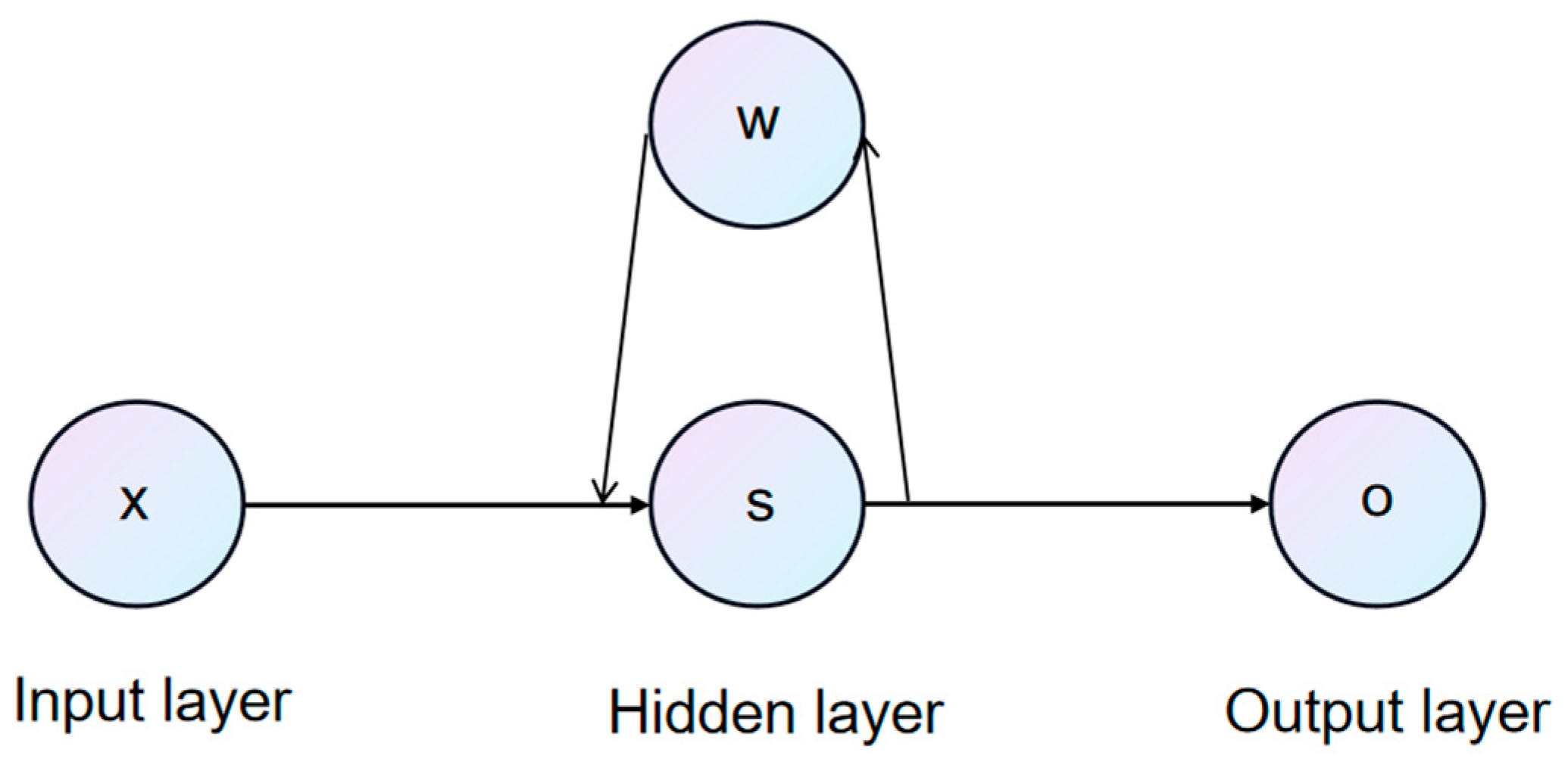
3.2.2. Recursive Neural Network (RNN)

The RNN structure illustrated in Figure 10 represents a kind of neural network with a memory function commonly used for processing sequence data, such as speech, text, etc.
The workflow of an RNN follows a sequential process that enables it to handle time-dependent data effectively. Initially, each element of the input sequence is fed into the network chronologically. At every time step, the network’s state is influenced by the current input, with the network computing its present state based on both the current input and its previous state. This state encapsulates information from all preceding moments, effectively serving as the network’s memory. The network then calculates the output for the current time step using the current state and input. Following this, the error between the output and the target value is computed and propagated back through the network using the backpropagation algorithm, which updates the network’s weight parameters. This process is repeated until the entire sequence has been processed. The distinguishing feature of RNNs is their ability to process sequence data of arbitrary length while considering contextual information within the sequence. This capability has led to their widespread applications, including speech recognition and time series prediction, where sequence data and temporal dependencies play important roles.
In a study by Fabio Biancofiore and colleagues [46], three distinct neural network models were employed to forecast mean PM10 levels for the upcoming one to three days. The methodologies encompassed a multivariate linear regression system, a recurrent neural network structure, and a feed-forward neural network configuration. Their research demonstrated that the recurrent neural network model surpassed both the multivariate linear regression system and the feed-forward neural network in performance. This outcome underscores the efficacy of RNNs in projecting PM2.5 and PM10 concentrations. An additional application of RNNs can be found in the development of encoder–decoder architectures.
L Petry et al. [47] used a sequence–sequence encoder–decoder model with RNN to predict air quality, and their predictions were highly consistent with field measurements. However, the model relied on a relatively narrow data source and would benefit from additional inputs such as weather, traffic, and satellite data. Long Short-Term Memory (LSTM) networks address the long-term dependency issue that general RNN models struggle with, making them more suitable for multi-variable time series prediction. Camilo Menares et al. [48] introduced various models for predicting the maximum PM2.5 concentration, including LSTM neural networks and Deep Feed-forward Neural Networks (DFFNNs), achieving excellent results with a seven-day memory window for LSTM. Endah Kristiani et al. [49] developed a haze prediction model that combined LSTM seq2seq with statistical methods, finding that the model trained on a single platform dataset performed more accurately than those trained on multiple platform datasets.
The DSRNN network, as a new recurrent neural network, adjusts the weights of time jump connections to achieve stability in cyclic hidden states, thereby alleviating the problems of gradient vanishing and explosion. [50] However, there are currently few studies using DSRNN.

3.2.3. Ensemble Model

Machine learning and deep learning methods face limitations in designing core functions, accounting for various weather factors, and providing timely and accurate long-term air quality predictions. In response to these challenges, the focus has shifted to multi-neural network hybrid models that combine multiple learning approaches.
Currently, a common hybrid approach involves combining CNN and LSTM networks, which have shown promising results. Zhendong Zhang et al. [51] developed VMDBiLSTM, a hybrid deep learning model that integrates Variational Mode Decomposition (VMD) with Bidirectional LSTM for predicting PM2.5 changes in Chinese cities. Their model decomposes PM2.5 spatial and temporal series into multiple sub-signal components using VMD and then uses BiLSTM to predict each sub-signal, significantly enhancing prediction accuracy. Qiang Sun et al. [52] introduced a hybrid Deep Air Quality Predictor that extracts shallow features using CNN, captures deep temporal features with LSTM, and uses Deep Neural Networks (DNNs) to convert these features into predictions. However, the model needs to incorporate spatial features and enhance precision for long-term air quality prediction. Similarly, Congcong Wen et al. [53] proposed a C-LSTME model, which combines CNN and LSTM, integrating PM2.5 data from highly correlated nearby stations to effectively extract additional temporal and spatial features. Table 3 summarizes more research involving ensemble models. Summarize the combination of models and their advantages and disadvantages.

4. Limitations and Future Directions

4.1. Issues and Improvement

Most existing air quality prediction models can produce satisfactory performance, but there are still some problems. We list them as follows:

4.1.1. The Curse of Dimension

In machine learning, when the spatial dimension increases, data sparsity, the predictive of the model decreases, and the demand for samples increases. Table 4 will provide a detailed description of these issues.
This is a great challenge for air quality prediction models. A potential approach to address this challenge was explored by Sang Won Choi and colleagues [63] in their 2021 study. They investigated the application of Principal Component Analysis (PCA) as a method to tackle high-dimensional issues. Utilizing Mean Absolute Error (MAE) and Root Mean Square Error (RMSE) as performance indicators, their research compared the efficacy of models with and without PCA implementation.
The findings of their study were noteworthy: models integrating PCA showed significant improvements in predictive accuracy. Specifically, there was an approximate 20% reduction in RMSE and a 33% decrease in MAE compared to models without PCA. These results strongly suggest that the incorporation of PCA techniques can substantially boost the effectiveness of deep learning architectures in handling multi-dimensional data.

4.1.2. The Interpretability of the Model

Model interpretability refers to the ability to clearly and clearly explain how a machine learning model makes predictions or decisions, as well as the aspects of input features that the model focuses on.
The interpretability of a model may be influenced by various factors, including model complexity, feature selection, data quality, algorithm type, and data volume.
  • Complexity: The relationship between a model’s sophistication and its transparency is often inverse. As models become more intricate, their inner workings become less clear. This is particularly evident in advanced architectures such as deep neural networks, where the sheer number of parameters—often in the millions—obscures the individual impact of each. Research by Eun Hun Lee and Hyeoncheol Kim [64] shed light on an interesting aspect of neural network training. They observed that effective learning involves not just the acquisition of repetitive units but also the development of complementary ones. These complementary units respond to identical inputs yet produce contrasting activation patterns. While this mechanism enhances the network’s capabilities, it introduces a layer of complexity when attempting to analyze the network’s decision-making process. The presence of these complementary elements can result in feature overlap, further complicating efforts to interpret the model’s behavior.
  • Feature selection: Feature selection can effectively improve the interpretability and computational feasibility of learning models, which is the reason why it is gradually favored [65]. If the model uses too many or too few features, its interpretability could decline. For example, if the model uses a large number of highly correlated features, it is hard for the model to determine which features are the most important. The crux of addressing the feature selection challenge lies in modeling the parameter–response relationships effectively. The primary objective is to identify the most parsimonious set of feature combinations that adequately capture these relationships. Several approaches address this issue, including wrapper-based feature selection [66], sparse regularization model-based feature selection [67,68,69], and kernel feature selection methods [70,71].
  • Data quality: Building and interpreting data visualization is critical to simplifying information access, improving data interpretability, and strengthening information literacy [72]. If there are errors or missing values in the training data, it may result in a reduction in the model’s interpretability.
  • Black box algorithms: Some algorithms, such as ANN and SVM, are called black box algorithms. Deep neural networks are well-known for their capability to handle a wide variety of machine learning and artificial intelligence tasks effectively. However, because of their highly parameterized and opaque nature, understanding the prediction results of these deep models can be quite challenging [73].
  • Data volume: If the training dataset is too small, it may lead to overfitting. When the dataset is too small, the model may try to remember the details of the training data without learning generalization rules, which can lead to poor performance on new data and may make it difficult for the model to explain. Much of the literature in recent years has expressed the importance of introducing additional data, such as topography, weather, and traffic, into the model. Canyang Guo et al. [60] conducted a detailed study on the relationship between humidity, air pressure, temperature, wind direction, and PM2.5 concentration, confirming that meteorological factors significantly influence air pollution levels.
The challenges posed by complex, opaque models are multifaceted and significant. When a model’s predictions lack explicability, it erodes user trust and confidence, potentially undermining its adoption and effectiveness. This opacity also complicates the debugging process, as pinpointing the source of errors within the model’s intricate architecture becomes a formidable task. Moreover, in heavily regulated sectors such as finance and healthcare, the inability to interpret model decisions can lead to non-compliance with regulatory standards that demand transparency and accountability. Perhaps most critically, the absence of clear interpretability hampers efforts to refine and enhance the model’s performance. Without a clear understanding of which factors drive the model’s output, researchers and developers face significant obstacles in identifying areas for improvement and optimization. Collectively, these issues underscore the pressing need for developing more interpretable AI models that balance complexity with transparency, ensuring both high performance and stakeholder trust.

4.1.3. The Utilization of the Internet of Things

The Internet of Things (IoT) has emerged as a transformative technology, integrating diverse sensors and communication systems to amass large amounts of data for myriad applications. In the context of smart city environments, IoT infrastructure serves as a cornerstone for developing sophisticated services that benefit both city management and residents [74]. However, it is crucial to acknowledge the significant disparity between developed and developing nations in terms of air quality monitoring devices, such as pollution sensors.
To address this gap, researchers are exploring ways to synergize IoT infrastructure with air quality prediction models, though this field remains in its nascent stages. For instance, Jovan Kalajdjieski and colleagues [75] innovated by incorporating uniform dataset cameras into their data collection process. Despite these advancements, the current landscape of air quality prediction predominantly relies on localized datasets, limiting the development of broadly applicable models with robust generalization capabilities.
In pursuit of more comprehensive solutions, Tien Huu Do et al. introduced an IoT-driven pipeline in Antwerp, Belgium, designed to collect, process, and visualize air pollution data. This framework utilizes IoT sensors installed on moving vehicles as well as fixed locations to monitor various urban environmental factors such as moisture levels in the air, ambient temperature, and atmospheric contaminants. The movement of vehicle-based measurements significantly expands the geographical coverage compared to static monitoring stations [74].
Further pushing the boundaries of IoT applications in air quality monitoring, L. Raja proposed an innovative technology that enables real-time data collection and transmission to servers in the cloud for analysis and decision-making. This approach, known as APM-OSSODL, has demonstrated superior performance metrics when compared to existing methodologies [76].
These developments underscore the potential of IoT in revolutionizing air quality monitoring and prediction, offering promising avenues for creating more comprehensive and accurate models that can address the global challenges of air pollution.
In addition, several algorithms have been proposed to enhance the efficiency and performance of air quality prediction models. Congcong Wen et al. [53] first used the EEMD algorithm to decompose the PM2.5 sequence from high to low into several IMF and then used three neural network combinations (BP, LSTM, CNN + LSTM) for training and prediction, effectively solving the prediction of PM2.5 concentration in heavy pollution seasons. In a study by Muhammad Hatta and colleagues [77], three distinct neural network architectures were employed to forecast indoor particulate matter levels. Their findings corroborated that the outdoor environment serves as the main contributor to indoor PM2.5 concentrations.

4.2. Future Directions, Trends, Challenges

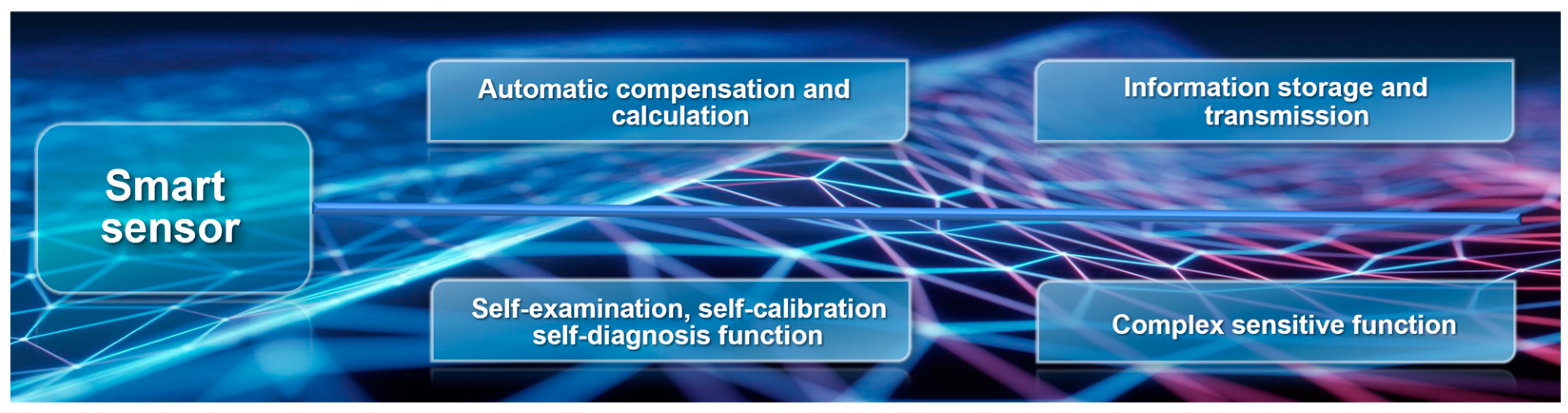
4.2.1. Using Smart Sensors

As an important part of any modern equipment in the 21st century, sensors also act as a key component in collecting air pollution data. Traditional sensing systems typically monitor the output of a single sensor, such as a varistor whose output resistance varies with pressure. However, the number of sensors in today’s equipment is gradually increasing. The increased data throughput presents significant challenges for information processing. Smart sensors with wireless technology, battery-free technology, machine learning, and other technologies are gradually replacing the position of traditional sensors and will play an excellent role in air pollution forecasts. Figure 11 shows the advantage of smart sensors. Marzena Banach et al. [78] developed small and inexpensive wireless smart sensors that integrate data processing units with artificial neural networks. These wireless sensor networks can be utilized to map dense air pollution in urban areas, contributing to the development of smart cities. What’s more, to cut costs and reduce the hassle of regular replacement. Thang Viet Tran and collaborators [79] introduced an innovative air quality monitoring device for indoor spaces. This sensor module operates without a battery and incorporates a radio frequency energy harvesting component.

4.2.2. Adapt to Other Key Pollutants

The machine learning method is worthy of recognition in air quality prediction, as it overcomes the non-linear barriers and uncertainties of air pollution. Recent studies [80,81,82] have shown that the model’s accuracy in predicting other key components of air, such as CO and NOx, remains limited. Additionally, these models are less accurate in predicting extreme concentrations of atmospheric pollutants. It is worth trying to enhance the model’s sensitivity to predict pollutant peak value and key pollutant concentration in the future.

4.2.3. Monitor the Concentration of Nanoparticles

Compared with particles such as PM2.5, nanoparticles are harmful because they enter the cardiovascular system in very large numbers and repeatedly attack and damage the blood vessels, which can eventually lead to heart attacks and strokes [83]. The influence of inhaled particulate matter (PM) on the cardiovascular system is the reason why air pollution results in high incidence rates and mortality. In urban areas, tiny particles, particularly those emitted by diesel engines, constitute a primary source of nanoparticles. These microscopic pollutants are especially concerning due to their adverse effects on human health [84]. However, the formation and prediction of nanoparticles in air have not been adequately studied, and most cities lack facilities to predict concentrations of nanoparticles. Therefore, Abdullah N. To address this, Abdullah N. AleDabbous et al. [85] combined a feed-forward artificial neural network with a backpropagation algorithm to develop a model. They determined the high pollution model through trial and error and comparative methods, using the 75th percentile values to evaluate predictions. Their findings indicate that nanoparticle concentration is highly sensitive to meteorological factors.

5. Conclusions

This paper mainly introduces the research status of earth science, air quality prediction, and air quality assessment. We found that ARTIFICIAL intelligence, especially machine learning and deep learning technology, has been extensively utilized and integrated in air quality forecast, including indoor and outdoor PM2.5 concentration prediction and improving traffic environments by using air pollution data. At the same time, through the cluster analysis of literature, we find that the hybrid model and spatio-temporal characteristics are the hot fields at present. This paper is beneficial to researchers and scholars in this field, helping them to identify future research directions and potential research gaps to guide their research efforts. Our vision for the future is as follows: (1) The application of intelligent sensors combined with machine learning and wireless technology in air prediction models needs to be expanded. (2) Using artificial intelligence to predict nanoparticles is an almost empty field. (3) The machine learning model’s sensitivity to air pollution peaks needs to improve in the future. In addition, we believe that enhancing the model’s generalization capacity is necessary. That is, a widely applicable dataset is very much needed. The model should include multiple sources of data, such as local wind direction, site density, and PM2.5 concentration in surrounding countries.

Author Contributions

Conceptualization, W.Z., L.Y. and L.W.; methodology, C.W., S.L. and J.T.; software, C.W. and J.T.; validation, S.L., L.Y. and J.T.; formal analysis, C.W. and L.W.; investigation, C.W. and W.Z.; resources, L.Y. and L.W.; data curation, C.W. and J.T.; writing—original draft preparation, C.W., L.Y. and W.Z.; writing—review and editing, C.W., J.T and W.Z.; visualization, S.L. and C.W.; supervision, L.W.; project administration, W.Z.; funding acquisition, W.Z. All authors have read and agreed to the published version of the manuscript.

Funding

Support by Sichuan Science and Technology Program (2023YFSY0026, 2023YFH0004).

Institutional Review Board Statement

Not applicable.

Informed Consent Statement

Not applicable.

Data Availability Statement

No new data were created or analyzed in this study.

Conflicts of Interest

The authors declare no conflict of interest.

References

  1. Zheng, T.; Wang, Y.; Zhou, Z.; Chen, S.; Jiang, J.; Chen, S. PM2.5 Causes Increased Bacterial Invasion by Affecting HBD1 Expression in the Lung. J. Immunol. Res. 2024, 2024, 6622950. [Google Scholar] [CrossRef] [PubMed]
  2. Mokhtar, S.B.; Viljoen, J.; van der Kallen, C.J.; Berendschot, T.T.; Dagnelie, P.C.; Albers, J.D.; Soeterboek, J.; Scarpa, F.; Colonna, A.; van der Heide, F.C. Greater exposure to PM2.5 and PM10 was associated with lower corneal nerve measures: The Maastricht study-a cross-sectional study. Environ. Health 2024, 23, 70. [Google Scholar] [CrossRef] [PubMed]
  3. Min, K.B.; Min, J.Y. Association of Ambient Particulate Matter Exposure with the Incidence of Glaucoma in Childhood. Am. J. Ophthalmol. 2020, 211, 176–182. [Google Scholar] [CrossRef] [PubMed]
  4. Qiao, H.; Xue, W.T.; Li, L.; Fan, Y.; Xiao, L.; Guo, M.M. Atmospheric Particulate Matter 2.5 (PM2.5) Induces Cell Damage and Pruritus in Human Skin. Biomed. Environ. Sci. 2024, 37, 216–220. [Google Scholar]
  5. Li, M.; Tang, B.; Zheng, J.; Luo, W.; Xiong, S.; Ma, Y.; Ren, M.; Yu, Y.; Luo, X.; Mai, B. Typical organic contaminants in hair of adult residents between inland and coastal capital cities in China: Differences in levels and composition profiles, and potential impact factors. Sci. Total Environ. 2023, 869, 161559. [Google Scholar] [CrossRef]
  6. Paik, K.; Na, J.-I.; Huh, C.-H.; Shin, J.-W. Particulate Matter and Its Molecular Effects on Skin: Implications for Various Skin Diseases. Int. J. Mol. Sci. 2024, 25, 9888. [Google Scholar] [CrossRef]
  7. Gan, T.; Bambrick, H.; Tong, S.L.; Hu, W.B. Air pollution and liver cancer: A systematic review. J. Environ. Sci. 2023, 126, 817–826. [Google Scholar] [CrossRef]
  8. Jiang, R.; Qu, Q.; Wang, Z.; Luo, F.; Mou, S. Association between air pollution and bone mineral density: A Mendelian randomization study. Arch. Med. Sci. 2024, 20, 1334–1338. [Google Scholar] [CrossRef]
  9. Zhang, F.; Zhu, S.; Di, Y.; Pan, M.; Xie, W.; Li, X.; Zhu, W. Ambient PM2.5 components might exacerbate bone loss among middle-aged and elderly women: Evidence from a population-based cross-sectional study. Int. Arch. Occup. Environ. Health 2024, 97, 855–864. [Google Scholar] [CrossRef]
  10. Yang, Y.; Li, R.; Cai, M.; Wang, X.J.; Li, H.P.; Wu, Y.L.; Chen, L.; Zou, H.T.; Zhang, Z.L.; Li, H.T.; et al. Ambient air pollution, bone mineral density and osteoporosis: Results from a national population-based cohort study. Chemosphere 2023, 310, 8. [Google Scholar] [CrossRef]
  11. Park, S.Y.; Han, J.; Kim, S.H.; Suk, H.W.; Park, J.E.; Lee, D.Y. Impact of Long-Term Exposure to Air Pollution on Cognitive Decline in Older Adults Without Dementia. J. Alzheimers Dis. 2022, 86, 553–563. [Google Scholar] [CrossRef] [PubMed]
  12. Yadav, V.K.; Bijekar, S.; Gacem, A.; Alkahtani, A.M.; Yadav, K.K.; Alreshidi, M.A.; Kumar, P.; Ghosh, T.; Verma, R.K.; Mishra, S. The impact of fine particulate matters (PM10, PM2.5) from incense smokes on the various organ systems: A review of an invisible killer. Part. Part. Syst. Charact. 2024, 41, 2300157. [Google Scholar] [CrossRef]
  13. Liu, J.; Song, R.; Li, X.; Liu, L.; Wei, N.; Yuan, J.; Yi, W.; Pan, R.; Cheng, J.; Zhang, X. Effects of PM2.5 and Its Components on Disease Severity in Patients with Schizophrenia and the Mediating Role of Thyroid Hormones. Environ. Health 2024, 2, 290–300. [Google Scholar] [CrossRef]
  14. Ran, Z.; Yang, J.; Liu, L.; Wu, S.; An, Y.; Hou, W.; Cheng, T.; Zhang, Y.; Zhang, Y.; Huang, Y. Chronic PM2.5 Exposure Disrupts Intestinal Barrier Integrity via Microbial Dysbiosis-Triggered TLR2/5-MyD88-NLRP3 Inflammasome Activation. Environ. Res. 2024, 258, 119415. [Google Scholar] [CrossRef]
  15. Xu, J.; Wang, J.; He, Y.; Chen, R.; Meng, Q.L. acidophilus participates in intestinal inflammation induced by PM2.5 through affecting the Treg/Th17 balance. Environ. Pollut. 2024, 341, 122977. [Google Scholar] [CrossRef]
  16. Tamashiro, L.K.; Yariwake, V.Y.; Veras, M.M.; Bertolla, R.P.; Intasqui, P. Fine inhalable particulate matter (PM2.5) present in air pollution and its effects on male germ cells chromatin packaging. Fertil. Steril. 2023, 120, e213–e214. [Google Scholar] [CrossRef]
  17. Zhang, X.; Wu, S.; Lu, Y.; Qi, J.; Li, X.; Gao, S.; Qi, X.; Tan, J. Association of ambient PM2.5 and its components with in vitro fertilization outcomes: The modifying role of maternal dietary patterns. Ecotoxicol. Environ. Saf. 2024, 282, 116685. [Google Scholar] [CrossRef]
  18. Tian, Y.; Ma, Y.; Wu, J.; Wu, Y.; Wu, T.; Hu, Y.; Wei, J. Ambient PM2.5 Chemical Composition and Cardiovascular Disease Hospitalizations in China. Environ. Sci. Technol. 2024, 58, 16327–16335. [Google Scholar] [CrossRef]
  19. Chanda, F.; Lin, K.-X.; Chaurembo, A.I.; Huang, J.-Y.; Zhang, H.-J.; Deng, W.-H.; Xu, Y.-J.; Li, Y.; Fu, L.-D.; Cui, H.-D. PM2.5-mediated cardiovascular disease in aging: Cardiometabolic risks, molecular mechanisms and potential interventions. Sci. Total Environ. 2024, 954, 176255. [Google Scholar] [CrossRef]
  20. Zhao, L.; Li, Z.; Qu, L. A novel machine learning-based artificial intelligence method for predicting the air pollution index PM2.5. J. Clean. Prod. 2024, 468, 143042. [Google Scholar] [CrossRef]
  21. Goodman, N.; Nematollahi, N.; Agosti, G.; Steinemann, A. Evaluating air quality with and without air fresheners. Air Qual. Atmos. Health 2020, 13, 1–4. [Google Scholar] [CrossRef]
  22. Lee, J.; Noh, J.H.; Noh, K.C.; Kim, Y.W.; Yook, S.J. Effect of a System Air Conditioner on Local Air Quality in a Four-bed Ward. Aerosol and Air Qual. Res. 2021, 21, 15. [Google Scholar] [CrossRef]
  23. Ma, Q.; Yuan, R.; Wang, S.; Sun, Y.; Zhang, Q.; Yuan, X.; Wang, Q.; Luo, C. Indigenized Characterization Factors for Health Damage Due to Ambient PM2.5 in Life Cycle Impact Assessment in China. Environ. Sci. Technol. 2024, 58, 17320–17333. [Google Scholar] [CrossRef] [PubMed]
  24. Braszus, B.; Rietbrock, A.; Haberland, C.; Ryberg, T. AI based 1-D P-and S-wave velocity models for the greater alpine region from local earthquake data. Geophys. J. Int. 2024, 237, 916–930. [Google Scholar] [CrossRef]
  25. Ro, S.H.; Gong, J. Scalable approach to create annotated disaster image database supporting AI-driven damage assessment. Nat. Hazards 2024, 120, 11693–11712. [Google Scholar] [CrossRef]
  26. Abegaz, R.; Wang, F.; Xu, J. History, causes, and trend of floods in the U.S.: A review. Nat. Hazards 2024. [Google Scholar] [CrossRef]
  27. Ghomi, S.M.M.M.; Bidhendi, G.R.N.; Amiri, M.J.; Kudahi, S.N. The Deployment Modeling of Low-Cost Sensors for Urban Particulate Matter Monitoring: A Case Study for PM2.5 Monitoring in Tehran City. Int. J. Environ. Res. 2024, 18, 111. [Google Scholar] [CrossRef]
  28. Jain, V.; Mukherjee, A.; Banerjee, S.; Madhwal, S.; Bergin, M.H.; Bhave, P.; Carlson, D.; Jiang, Z.; Zheng, T.; Rai, P. A hybrid approach for integrating micro-satellite images and sensors network-based ground measurements using deep learning for high-resolution prediction of fine particulate matter (PM2.5) over an Indian city, Lucknow. Atmos. Environ. 2024, 338, 120798. [Google Scholar] [CrossRef]
  29. Das, T.; Talukdar, S.; Naikoo, M.W.; Ahmed, I.A.; Rahman, A.; Islam, M.K.; Alam, E. Integration of fuzzy AHP and explainable AI for effective coastal risk management: A micro-scale risk analysis of tropical cyclones. Prog. Disaster Sci. 2024, 23, 100357. [Google Scholar] [CrossRef]
  30. Longo, R.; Lacanna, G.; Innocenti, L.; Ripepe, M. Artificial Intelligence and Machine Learning tools for improving Early Warning systems of volcanic eruptions: The case of Stromboli. IEEE Trans. Pattern Anal. Mach. Intell. 2024, 46, 7973–7982. [Google Scholar] [CrossRef]
  31. Demir, E.; Cavur, M.; Yu, Y.-T.; Duzgun, H.S. An Evaluation of AI Models’ Performance for Three Geothermal Sites. Energies 2024, 17, 3255. [Google Scholar] [CrossRef]
  32. Liu, N.; Zou, B.; Li, Y.; Zang, Z.; Xu, S.; Li, S.; Li, S.; Zhi, L.; Chen, J.; Zhao, F. An Accurate and Efficient Forecast Framework for Fine PM2.5 Maps Using Spatiotemporal Recurrent Neural Networks. J. Clean. Prod. 2024, 475, 143624. [Google Scholar] [CrossRef]
  33. Balcone-Boissard, H.; Boudon, G.; Zdanowicz, G.; Orsi, G.; Webster, J.D.; Civetta, L.; D’Antonio, M.; Arienzo, I. The space-time architecture variation of the shallow magmatic plumbing systems feeding the Campi Flegrei and Ischia volcanoes (Southern Italy) from halogen constraints. Am. Mineral. 2024, 109, 977–991. [Google Scholar] [CrossRef]
  34. Choiruddin, A.; Rahman, A.A.; Andreas, C. Algorithms for Fitting the Space-Time ETAS Model to Earthquake Catalog Data: A Comparative Study. J. Agric. Biol. Environ. Stat. 2024, 1–18. [Google Scholar] [CrossRef]
  35. Li, Z.; Zhou, L.; Duan, M.; Zhao, C. Three-dimensional VP, VS, and VP/VS imaging based on AI microseismic detection reveals the mechanism of induced earthquakes in the Xiluodu Reservoir Area, China. J. Asian Earth Sci. 2024, 266, 106123. [Google Scholar] [CrossRef]
  36. Jin, W.X.; Luo, Y.; Wu, T.W.; Huang, X.M.; Xue, W.; Yu, C.Q. Deep Learning for Seasonal Precipitation Prediction over China. J. Meteorol. Res. 2022, 36, 271–281. [Google Scholar] [CrossRef]
  37. Pak, U.; Ma, J.; Ryu, U.; Ryom, K.; Juhyok, U.; Pak, K.; Pak, C. Deep learning-based PM2.5 prediction considering the spatiotemporal correlations: A case study of Beijing, China. Sci. Total Environ. 2020, 699, 11. [Google Scholar] [CrossRef]
  38. Liu, D.R.; Lee, S.J.; Huang, Y.; Chiu, C.J. Air pollution forecasting based on attention-based LSTM neural network and ensemble learning. Expert. Syst. 2020, 37, 16. [Google Scholar] [CrossRef]
  39. Hu, J.L.; Li, X.; Huang, L.; Ying, Q.; Zhang, Q.; Zhao, B.; Wang, S.X.; Zhang, H.L. Ensemble prediction of air quality using the WRF/CMAQ model system for health effect studies in China. Atmos. Chem. Phys. 2017, 17, 13103–13118. [Google Scholar] [CrossRef]
  40. Liao, Q.; Zhu, M.M.; Wu, L.; Pan, X.L.; Tang, X.; Wang, Z.F. Deep Learning for Air Quality Forecasts: A Review. Curr. Pollut. Rep. 2020, 6, 399–409. [Google Scholar] [CrossRef]
  41. Hafiz, A.M.; Hassaballah, M.; Binbusayyis, A. Formula-Driven Supervised Learning in Computer Vision: A Literature Survey. Appl. Sci. 2023, 13, 15. [Google Scholar] [CrossRef]
  42. Kang, Y.; Cai, Z.; Tan, C.W.; Huang, Q.; Liu, H.F. Natural language processing (NLP) in management research: A literature review. J. Manag. Anal. 2020, 7, 139–172. [Google Scholar] [CrossRef]
  43. Bekkar, A.; Hssina, B.; Douzi, S.; Douzi, K. Air-pollution prediction in smart city, deep learning approach. J. Big Data 2021, 8, 21. [Google Scholar] [CrossRef] [PubMed]
  44. Uzun Ozsahin, D.; Duwa, B.B.; Ozsahin, I.; Uzun, B. Quantitative Forecasting of Malaria Parasite Using Machine Learning Models: MLR, ANN, ANFIS and Random Forest. Diagnostics. 2024, 14, 385. [Google Scholar] [CrossRef]
  45. Hoffman, S.; Filak, M.; Jasinski, R. Air Quality Modeling with the Use of Regression Neural Networks. Int. J. Environ. Res. Public Health 2022, 19, 33. [Google Scholar] [CrossRef]
  46. Biancofiore, F.; Busilacchio, M.; Verdecchia, M.; Tomassetti, B.; Aruffo, E.; Bianco, S.; Di Tommaso, S.; Colangeli, C.; Rosatelli, G.; Di Carlo, P. Recursive neural network model for analysis and forecast of PM10 and PM2.5. Atmos. Pollut. Res. 2017, 8, 652–659. [Google Scholar] [CrossRef]
  47. Petry, L.; Meiers, T.; Reuschenberg, D.; Mirzavand Borujeni, S.; Arndt, J.; Odenthal, L. Design and Results of an Ai-Based Forecasting of Air Pollutants for Smart Cities. ISPRS Ann. Photogramm. Remote Sens. Spat. Inf. Sci. 2021, VIII-4/W1-2021, 89–96. [Google Scholar]
  48. Menares, C.; Perez, P.; Parraguez, S.; Fleming, Z.L. Forecasting PM2.5 levels in Santiago de Chile using deep learning neural networks. Urban Clim. 2021, 38, 100906. [Google Scholar] [CrossRef]
  49. Kristiani, E.; Kuo, T.-Y.; Yang, C.-T.; Pai, K.-C.; Huang, C.-Y.; Nguyen, K.L.P. PM2.5 Forecasting Model Using a Combination of Deep Learning and Statistical Feature Selection. IEEE Access 2021, 9, 68573–68582. [Google Scholar] [CrossRef]
  50. Saab, S.; Fu, Y.W.; Ray, A.; Hauser, M. A Dynamically Stabilized Recurrent Neural Network. Neural Process. Lett. 2022, 54, 1195–1209. [Google Scholar] [CrossRef]
  51. Zhang, Z.; Zeng, Y.; Yan, K. A hybrid deep learning technology for PM2.5 air quality forecasting. Environ. Sci. Pollut. Res. Int. 2021, 28, 39409–39422. [Google Scholar] [CrossRef]
  52. Sun, Q.; Zhu, Y.; Chen, X.; Xu, A.; Peng, X. A hybrid deep learning model with multi-source data for PM2.5 concentration forecast. Air Qual. Atmos. Health 2020, 14, 503–513. [Google Scholar] [CrossRef]
  53. Wen, C.; Liu, S.; Yao, X.; Peng, L.; Li, X.; Hu, Y.; Chi, T. A novel spatiotemporal convolutional long short-term neural network for air pollution prediction. Sci. Total Environ. 2019, 654, 1091–1099. [Google Scholar] [CrossRef] [PubMed]
  54. Yeo, I.; Choi, Y.; Lops, Y.; Sayeed, A. Efficient PM2.5 forecasting using geographical correlation based on integrated deep learning algorithms. Neural Comput. Appl. 2021, 33, 15073–15089. [Google Scholar] [CrossRef]
  55. Faraji, M.; Nadi, S.; Ghaffarpasand, O.; Homayoni, S.; Downey, K. An integrated 3D CNN-GRU deep learning method for short-term prediction of PM2.5 concentration in urban environment. Sci. Total Environ. 2022, 834, 12. [Google Scholar] [CrossRef]
  56. Guo, Z.Y.; Yang, C.Y.; Wang, D.S.; Liu, H.B. A novel deep learning model integrating CNN and GRU to predict particulate matter concentrations. Process Saf. Environ. Protect. 2023, 173, 604–613. [Google Scholar] [CrossRef]
  57. Hu, J.T.; Chen, Y.Y.; Wang, W.; Zhang, S.C.; Cui, C.; Ding, W.K.; Fang, Y. An optimized hybrid deep learning model for PM2.5 and O-3 concentration prediction. Air Qual. Atmos. Health 2023, 16, 857–871. [Google Scholar] [CrossRef]
  58. Li, D.; Liu, J.P.; Zhao, Y.Y. Prediction of Multi-Site PM2.5 Concentrations in Beijing Using CNN-Bi LSTM with CBAM. Atmosphere 2022, 13, 19. [Google Scholar] [CrossRef]
  59. Tong, W.T.; Li, L.X.; Zhou, X.L.; Hamilton, A.; Zhang, K. Deep learning PM2.5 concentrations with bidirectional LSTM RNN. Air Qual. Atmos. Health 2019, 12, 411–423. [Google Scholar] [CrossRef]
  60. Guo, C.Y.; Liu, G.G.; Chen, C.H. Air Pollution Concentration Forecast Method Based on the Deep Ensemble Neural Network. Wirel. Commun. Mob. Comput. 2020, 2020, 13. [Google Scholar] [CrossRef]
  61. Wang, J.Y.; Li, J.Z.; Wang, X.X.; Wang, J.; Huang, M. Air quality prediction using CT-LSTM. Neural Comput. Appl. 2021, 33, 4779–4792. [Google Scholar] [CrossRef]
  62. Qiao, W.B.; Tian, W.C.; Tian, Y.; Yang, Q.; Wang, Y.N.; Zhang, J.Z. The Forecasting of PM2.5 Using a Hybrid Model Based on Wavelet Transform and an Improved Deep Learning Algorithm. IEEE Access 2019, 7, 142814–142825. [Google Scholar] [CrossRef]
  63. Choi, S.; Kim, B. Applying PCA to Deep Learning Forecasting Models for Predicting PM2.5. Sustainability 2021, 13, 3726. [Google Scholar] [CrossRef]
  64. Lee, E.H.; Kim, H. Feature-Based Interpretation of the Deep Neural Network. Electronics 2021, 10, 20. [Google Scholar] [CrossRef]
  65. Barraza, J.F.; Droguett, E.L.; Martins, M.R. Towards Interpretable Deep Learning: A Feature Selection Framework for Prognostics and Health Management Using Deep Neural Networks. Sensors 2021, 21, 30. [Google Scholar] [CrossRef] [PubMed]
  66. Kumar, R. Composition of Feature Selection for Time-Series Prediction with Deep Learning. Procedia Comput. Sci. 2024, 235, 1477–1488. [Google Scholar]
  67. Wu, W.-B.; Chen, S.-B.; Ding, C.; Luo, B. Non-linear Feature Selection Based on Convolution Neural Networks with Sparse Regularization. Cogn. Comput. 2024, 16, 654–670. [Google Scholar] [CrossRef]
  68. Sun, Z.; Chen, Z.; Liu, J.; Yu, Y. Multi-class feature selection via Sparse Softmax with a discriminative regularization. Int. J. Mach. Learn. Cybern. 2024, 1–14. [Google Scholar] [CrossRef]
  69. Li, Y.; Zhang, Y.; Wu, J.; Xie, M. Regularized Periodic Gaussian Process for Nonparametric Sparse Feature Extraction From Noisy Periodic Signals. IEEE Trans. Autom. Sci. Eng. 2024, 1–10. [Google Scholar] [CrossRef]
  70. Tang, Z.; Wang, S.; Li, Y. Dynamic NOX emission concentration prediction based on the combined feature selection algorithm and deep neural network. Energy 2024, 292, 130608. [Google Scholar] [CrossRef]
  71. Zheng, W.; Zhu, X.F.; Wen, G.Q.; Zhu, Y.H.; Yu, H.; Gan, J.Z. Unsupervised feature selection by self-paced learning regularization. Pattern Recognit. Lett. 2020, 132, 4–11. [Google Scholar] [CrossRef]
  72. de Foy, B.; Edwards, R.; Joy, K.S.; Zaman, S.U.; Salam, A.; Schauer, J.J. Interpretable machine learning tools to analyze PM2.5 sensor network data so as to quantify local source impacts and long-range transport. Atmos. Res. 2024, 311, 107656. [Google Scholar] [CrossRef]
  73. Rakholia, R.; Le, Q.; Vu, K.; Ho, B.Q.; Carbajo, R.S. Accurate PM2.5 urban air pollution forecasting using multivariate ensemble learning Accounting for evolving target distributions. Chemosphere 2024, 364, 143097. [Google Scholar] [CrossRef]
  74. Purnomo, A.; Badriah, S.; Andang, A.; Gunawan, M.R.; Maulana, D.I.; Sambas, A.; Madi, E.N. An Affordable Green IoT-Based System for Remote Sensing of PM1, PM2.5 and PM10 Particulate Matter. J. Adv. Res. Appl. Sci. Eng. Technol. 2024, 49, 134–148. [Google Scholar] [CrossRef]
  75. Kalajdjieski, J.; Zdravevski, E.; Corizzo, R.; Lameski, P.; Kalajdziski, S.; Pires, I.M.; Garcia, N.M.; Trajkovik, V. Air Pollution Prediction with Multi-Modal Data and Deep Neural Networks. Remote Sens. 2020, 12, 4142. [Google Scholar] [CrossRef]
  76. Raja, L.; Maheswaravenkatesh, P.; Shanthi, G.; Surya, G. Internet of things enabled automated air pollution monitoring using oppositional swallow swarm optimisation with deep learning model. J. Environ. Prot. Ecol. 2022, 23, 462–473. [Google Scholar]
  77. Hatta, M.; Han, H. Predicting indoor PM2.5/PM10 concentrations using simplified neural network models. J. Mech. Sci. Technol. 2021, 35, 3249–3257. [Google Scholar] [CrossRef]
  78. Banach, M.; Talaśka, T.; Dalecki, J.; Długosz, R. New technologies for smart cities—High-resolution air pollution maps based on intelligent sensors. Concurr. Comput. Pract. Exp. 2019, 32, e5179. [Google Scholar] [CrossRef]
  79. Tran, T.V.; Dang, N.T.; Chung, W.-Y. Battery-free smart-sensor system for real-time indoor air quality monitoring. Sens. Actuators B Chem. 2017, 248, 930–939. [Google Scholar] [CrossRef]
  80. Liu, B.C.; Binaykia, A.; Chang, P.C.; Tiwari, M.K.; Tsao, C.C. Urban air quality forecasting based on multi-dimensional collaborative Support Vector Regression (SVR): A case study of Beijing-Tianjin-Shijiazhuang. PLoS ONE 2017, 12, e0179763. [Google Scholar] [CrossRef]
  81. Nieto, P.J.; Anton, J.C.; Vilan, J.A.; Garcia-Gonzalo, E. Air quality modeling in the Oviedo urban area (NW Spain) by using multivariate adaptive regression splines. Environ. Sci. Pollut. Res. Int. 2015, 22, 6642–6659. [Google Scholar] [CrossRef]
  82. Philibert, A.; Loyce, C.; Makowski, D. Prediction of N2O emission from local information with Random Forest. Environ. Pollut. 2013, 177, 156–163. [Google Scholar] [CrossRef]
  83. Rybarczyk, Y.; Zalakeviciute, R. Machine Learning Approaches for Outdoor Air Quality Modelling: A Systematic Review. Appl. Sci. 2018, 8, 2570. [Google Scholar] [CrossRef]
  84. Yao, Q.; Shi, J.; Han, X.; Tian, S.; Huang, J.; Li, Y.; Ning, P. Emissions of polycyclic aromatic hydrocarbons in PM2.5 emitted from motor vehicles exhaust (PAHs-PM2.5-MVE) under the plateau with low oxygen content. Atmos. Environ. 2024, 321, 120364. [Google Scholar] [CrossRef]
  85. Al–Dabbous, A.N.; Kumar, P.; Khan, A.R. Prediction of airborne nanoparticles at roadside location using a feed–forward artificial neural network. Atmos. Pollut. Res. 2017, 8, 446–454. [Google Scholar] [CrossRef]
Figure 1. The harm of PM2.5 to the human body. (By Figdraw, ID: RUAYW6307d).
Atmosphere 15 01411 g001
Figure 2. Characteristics of Earth Science Data.
Atmosphere 15 01411 g002
Figure 3. Four Major Applications of Artificial Intelligence in Earth Science.
Atmosphere 15 01411 g003
Figure 4. Development trend of literature and its percentage in total literature from 2012 to 2023.
Atmosphere 15 01411 g004
Figure 5. Research topic co-occurrence network.
Atmosphere 15 01411 g005
Figure 6. Keyword co-occurrence network.
Atmosphere 15 01411 g006
Figure 7. Keyword clustering result.
Atmosphere 15 01411 g007
Figure 8. Clustering timeline diagram.
Atmosphere 15 01411 g008
Figure 9. The development process of artificial neural network models is divided into eight steps.
Atmosphere 15 01411 g009
Figure 10. Simple recurrent neural networks.
Atmosphere 15 01411 g010
Figure 11. The advantage of smart sensors.
Atmosphere 15 01411 g011
Table 1. The top 10 most cited journals.
Number.JournalCountsCiteScoreIF
(2022)
Publishers
1Atmosphere424.103.9MDPI
2Atmospheric Pollution Research267.904.5TUNCAP
3Atmospheric
Environment
2510.305.755Elsevier
4Sustainability225.803.889MDPI
5Environmental
Pollution
1714.909.888Elsevier
5Environmental
Science and Pollution Research
177.905.19Springer Berlin Heidelberg
5Science of The Total Environment1716.809.8Elsevier
8IEEE Access159.003.476IEEE
8Urban Climate158.706.4Elsevier
10Aerosol and Air
Quality Research
147.304AAGR Aerosol and Air Quality Research
Table 2. 20 mutation keywords (Red represents the time of mutation emergence).
KeywordsYearStrengthBeginEnd2012–2023
Chemical Composition20124.776220152018Atmosphere 15 01411 i001
Ambient Air20124.262120132019Atmosphere 15 01411 i002
Particulate Air Pollution20124.068320122018Atmosphere 15 01411 i003
YangtzeRiver Delta20124.066320152019Atmosphere 15 01411 i004
Temporal Variation20123.894120142018Atmosphere 15 01411 i005
Source Apportionment20123.554520132015Atmosphere 15 01411 i006
Matter20123.504620172018Atmosphere 15 01411 i007
Urban20123.204120152016Atmosphere 15 01411 i008
Area20123.039820122016Atmosphere 15 01411 i009
Particle20122.898720122013Atmosphere 15 01411 i010
Seasonal Variation20122.87820142018Atmosphere 15 01411 i011
Aerosol20122.874220122018Atmosphere 15 01411 i012
Asthma20122.64720142016Atmosphere 15 01411 i013
System20122.591920192021Atmosphere 15 01411 i014
Modi20122.564720172018Atmosphere 15 01411 i015
Pm2.520122.515320212023Atmosphere 15 01411 i016
Trend20122.482320182019Atmosphere 15 01411 i017
Cohort20122.372320142016Atmosphere 15 01411 i018
Variability20122.20420182019Atmosphere 15 01411 i019
health20122.192720172018Atmosphere 15 01411 i020
Table 3. Several research related to ensemble models.
ModelAdvantagesDisadvantages
VMD & BiLSTM [51]In relation to current models, when evaluating the precision of forecasts and the capability to forecast tendencies accurately.Not applicable to other prediction fields.
CNN & GRU [54]Improve PM2.5 prediction accuracy. The average improvement is about 10%.Only applicable to predicting the concentration of PM2.5 not applicable to other pollutants.
3D
CNN & GRU [55]
Compared with recent methods such as LSTM, ANN, and ARIMA, this model can yield promising outcomes with a lower RMSE and MAE in the PM2.5 prediction environment.Data missing in the time series results in discontinuities in the data sequence and a decrease in long-term prediction ability.
RF & CNN & GRU [56]In the case of incomplete raw data, it can effectively predict the concentration of PM2.5 in the indoor environment, reducing the RMSE by between 22.35% and 36.75%, and the R2 improved by between 10.88% and 29.31%.The limited number of samples could potentially impact how well the model applies to more extensive data collection.
CNN &
BiLSTM & GRU & DNN [57]
It is a promising method for predicting the performance of atmospheric and particulate pollutants. In the case of single-source data, for PM2.5, this model’s MAE decreased between 18.9 and 27.4%, and the RMSE decreased between 6.9 and 23.7%. The R2 increased between 0.8 and 3.6%.Other factors, including traffic conditions and contaminants originating from pollution sources, are not considered and utilized.
CNN & LSTM [37]Compared with multi-layer perception (MLP) and LSTM models, this method exhibits enhanced stability and prediction performance. This model (RMSE 2.997, MAE 2.21, MAPE 0.039) has an obvious improvement as compared to LSTM (RMSE 4.764, MAE 3.612, MAPE 0.068).There was no attempt to limit the target site as the center method to the application scope of the target site itself or neighboring sites.
CNN&LSTM&DNN [52]This model outperforms other models in predicting PM2.5 concentration. In the case of the multi-source data, the forecasting errors of the HDAQP model are lower than RMSE, MAE, and MAPE, which are 23.935, 12.252, and 23.541, respectively.The HDAQP model’s forecasting accuracy tends to decline as it attempts to predict further into the future.
CBAM & CNN & BiLSTM [58]Overcoming the shortcomings of CNN-LSTM and the long-term dependence of PM2.5 concentration, it has greater practical value. In single-step PM2.5 concentration prediction, this model reduces RMSE to 18.90, MAE to 11.20, improves R2 to 0.9397, and IA to 98.54%.The study did not take into account vehicular movement, plant density, or foot traffic patterns.
LSTM & RNN [59]Spatiotemporal interpolated data of air pollutant concentrations can be used.They did not investigate the method of deploying the model onto a cluster computing framework to accelerate the process.
RNN & LSTM & GRU [60]This model has better generalization ability and prediction ability. MAE and MAPE of this model were 8.58 and 24.73%, respectively, better than CGRU (8.56 and 20.50%) and other models.
Compared with SGD, this model can effectively avoid local optima.
They lack research on the effects of human activities and terrain types on PM2.5.
CT & LSTM [61]Has high prediction accuracy. The prediction accuracy of the new method is 93.70%, which is 8.22% higher than that of the BP neural network method (85.48%).No research on multi-scale prediction in the spatial domain.
WT & SAE & LSTM [62]Determine the optimal wavelet layer and order different samples.
Improved the issue of LSTM gradient vanishing, resulting in better predictive performance than other models. The MAE of SAE-LSTM is between 0.1723 and 1.4574 lower than those of other models when applied to data from Xuchang.
Did not verify whether the algorithm in this study is applicable to other fields
Table 4. Description of dimension curse problem.
ProblemExplain
Data sparsityIn high-dimensional space, the distance between data points becomes farther, resulting in sparse data. This means that in high-dimensional space, the similarity between data points becomes more blurred, posing challenges for the model to distinguish different data points accurately.
The predictive ability of the model has decreased.As the number of spatial dimensions grows, the model’s complexity escalates correspondingly. This increased complexity raises the likelihood of overfitting, potentially compromising the prediction performance of the model. Moreover, the sparsity of data points in higher-dimensional spaces can lead to a decline in the model’s capacity to generalize effectively.
The demand for samples has increased.In multi-dimensional environments, achieving model precision requires training samples to cover the feature space more comprehensively. Consequently, higher-dimensional problems demand larger datasets to effectively train and calibrate an accurate model. This phenomenon underscores the need for wider data sampling and processing in complex spatial prediction tasks.
Disclaimer/Publisher’s Note: The statements, opinions and data contained in all publications are solely those of the individual author(s) and contributor(s) and not of MDPI and/or the editor(s). MDPI and/or the editor(s) disclaim responsibility for any injury to people or property resulting from any ideas, methods, instructions or products referred to in the content.

