Analysis of ENSO Event Intensity Changes and Time–Frequency Characteristic Since 1875

Abstract

This study investigates the characteristics and intensity of El Niño–Southern Oscillation (ENSO) events from January 1875 to December 2023, employing an advanced method for intensity determination based on various ENSO indices defined as a continuous five-month period with temperatures exceeding 0.5 °C for warm events or falling below −0.5 °C for cold events. A total of 40 warm and 41 cold events were identified, with further classification revealing seven extreme warm events and five extreme cold events. The analysis shows a positive skewness in frequency distribution, indicating a predominance of strong warm events. The primary mode of variability is found to be interannual oscillation in the 3–8 year range, with significant decadal oscillations in the 10–16 year range. This study highlights the importance of methodological rigor in evaluating ENSO dynamics, contributing to a more comprehensive understanding of climate variability and offering a reliable framework for future research.

1. Introduction

ENSO is a periodic fluctuation in sea surface temperature (SST) and atmospheric pressure in the equatorial Pacific, characterized by a distinct cyclical pattern, and is thus also referred to as the ENSO cycle [1,2]. El Niño refers to the abnormal warming of SST in the Central and Eastern equatorial Pacific, while the Southern Oscillation (SO) refers to the difference in sea-level pressure (SLP) across the tropical Pacific. Together, they form the ENSO, occurring irregularly every 2 to 7 years [3]. As the largest interannual signal originating from an ocean–atmosphere coupling in the tropical Pacific, ENSO significantly impacts weather and climate around the world [4].

ENSO events have been a key research topic in climate science, involving major climate change phenomena occurring in the equatorial Pacific region [5]. Bjerknes and Jacob [6] were the first to explain the physical relationship and dynamic mechanism between the Southern Oscillation and El Niño. Rasmusson et al. [7] defined a typical El Niño phenomenon, where abnormal sea surface warming originates off the coast of South America and spreads westward across the equatorial Pacific. Over the past few decades, extensive and in-depth research on ENSOs has been conducted, leading to significant advancements in ENSO studies [1,4,8]. Before the 1960s, El Niño and the SO were analyzed as two separate signals in the ocean and atmosphere, respectively, based on limited observational data, identifying some basic characteristics of interannual anomalies in sea temperature and surface atmospheric fields (e.g., SLP) [9]. In the late 1960s, it was recognized that El Niño and the SO are closely related aspects of the same large-scale ocean–atmosphere interaction process in the tropical Pacific [5,6,7], marking the beginning of a new era where these two phenomena were studied as a whole, shifting from simple statistical analysis to dynamic diagnostic analysis.

The definition and intensity classification of ENSO events have been hot topics of research in recent years. Quinn et al. [10] were the first to establish a list of El Niño events and categorized them into four levels: extremely weak, weak, moderate, and strong, but the definition and representation of El Niño intensity were limited to ordinal scales. Conventionally, ENSO characteristics and evolution are represented by SST data, primarily using SST in Niño 3, Niño 4, and Niño 3.4 regions. The start and end times, intensity levels, and types of ENSO events have been classified using the maximum and minimum SST anomalies (SSTAs), with ENSO events categorized into five levels: extremely weak, weak, moderate, strong, and extremely strong, using corresponding indices to determine event types [11]. Wang et al. [12] used SST sequences from Niño 3 and Niño 4 regions along with two Southern Oscillation Index (SOI) sequences, considering both SST and the SOI, to establish a seasonal-scale ENSO index series from 1867 to 1998, evaluating each event’s intensity as weak, moderate, or strong. Li and Zhai [13] weighted the SST anomalies in Niño 1+2, Niño 3, and Niño 4 regions by their respective area proportions to derive a comprehensive Niño region SST anomaly index, using this index to define ENSO events from 1951 to 1996 and introduce a composite index for the strength of ocean–atmosphere interaction during ENSO events.

In recent studies, Tedeschi and Sampaio [14] have proposed defining the intensity of ENSO events based on seasonal variations rather than annual measures, arguing that seasonal intensity is crucial for seasonal forecasting. Unlike the typical annual classification, seasonal intensity better captures the impact of ENSOs on climate. Dieppois et al. [15] identified significant decadal variability in both the intensity and location of ENSO events using long-term observational data. Feng et al. [16] employed a rotated principal component analysis (RPCA) to reveal that El Niño events can be described by three primary Pacific SST modes, introducing Central Pacific Variability (CPV) as an important factor for characterizing ENSO intensity. Emmanuel [17] explored the correlation between ENSO indices and precipitation anomalies using both parametric and non-parametric methods, discussing how precipitation anomalies can be used to define and classify different intensities of El Niño and La Niña events. Zhou and Wang [18] utilized wavelet decomposition methods to define ENSO events, emphasizing how frequency components of SST anomalies can be used to assess ENSO event intensity. By decomposing the SST time series, their study enables the identification of ENSO events at different periods and quantitatively evaluates their intensity. Cerón et al. [19] investigated the time variation in ENSO variability in the tropical Pacific using wavelet transforms and a frequency analysis, exploring how the intensity of ENSO events shifts over time across different frequency components. Kido et al. [20] simulated ENSO phenomena using coupled climate models and evaluated ENSO intensity and frequency through simulated SST and precipitation changes. Their work discussed the comparison between model simulations and observational data, providing insights into how climate models perform in forecasting the intensity of ENSO events.

At the same time, many researchers have studied the interannual and decadal oscillations of ENSO. Wang [21,22] found that the climate shift around 1977 altered the mean climate state of ENSO events, influencing the frequency and mode changes in ENSO events, manifesting in an increased frequency and intensity of ENSO events [23]. Wang et al. [24] analyzed the interannual and decadal variations in the SO using Morlet wavelet transform and Gabor wavelet transform, discovering a significant shift in the main period of the SO in the mid-1960s. Between 1911 and 1960, the main period of the SO was 5–7 years, while, from 1970 to 1992, the main period was around 5 years. The amplitude of the SO also varied significantly, being weakest in the 1960s and strongest from 1970 to 1992. Torrence et al. [25,26,27] analyzed indices such as Niño 3 and the SOI and found that El Niño and La Niña occurred approximately every 2–7 years, corresponding to the ENSO cycle, and that this oscillation exhibited a decadal variation of 12–20 years. From 1920 to 1950, ENSO variance was at a low level, while, from 1960 to 1990, ENSO variance was at a high level. Zhang and Din [28] used Niño 3 and Niño 4 indices and, through a wavelet analysis, defined signals in the 2–7 year frequency range as ENSO modes, with signals in the 8–20 year range regarded as decadal variations in the ENSO.

The main indices used to characterize ENSO events include the equatorial Pacific sea surface temperature indices (such as Niño 1+2, Niño 3, Niño 4, Niño 3.4), the SOI, and the Multivariate ENSO Index (MEI). Recent studies have tended to use multiple indicators to define ENSO events, as the ENSO involves multiple aspects of the ocean–atmosphere system. Using only SST indices or SOIs from the equatorial Pacific alone cannot fully represent ENSO events [29]. This paper utilizes the latest data for the ONI, SOI, and MEI and combines various analysis methods from previous studies to determine ENSO events and their indices from 1875 to 2023, exploring both the interannual and decadal variations in the ENSO.

2. Materials and Methods

2.1. Data

This study utilized the following datasets:

• Niño Index Data: Provided by the Climate Prediction Center (CPC) of the U.S. National Centers for Environmental Prediction (NCEP), based on the HadiSST v1.1 dataset [30]. The Niño3.4 index was calculated from SST data for the region 170°W–120°W, 5°N–5°S, covering the period from 1870 to the present. The Niño3 index, calculated from the SST dataset for the region 150°W–90°W, 5°N–5°S, spans the same time period. The Niño4 index was also calculated from the SST dataset for the region 160°E–150°W, 5°N–5°S. The Oceanic Niño Index (ONI) was calculated as the three-month running average of SST anomalies in the Niño3.4 region, using the HadiSST v1.1 dataset, with data available from 1870 onward. The Niño 1+2 index is one of Niño indices that was mainly used to monitor the initial changes in ENSO events, reflecting the sea surface temperature anomalies in the Eastern Pacific, closest to South America. The SST fluctuations in this region are more susceptible to local climatic phenomena (such as tropical storms, monsoons, etc.). Therefore, changes in this index may reflect more local weather patterns rather than the intensity and persistence of ENSO events on a global scale. As a result, we did not consider using this index in our research.
• SOI Data: Provided by the CPC, covering the period from 1866 to the present. The SOI was calculated by first standardizing the sea-level pressure data from Tahiti and Darwin, then taking the difference (Standardized Tahiti—Standardized Darwin) and dividing it by the monthly standard deviation (MSD).
• MEI Data: Provided by the Physical Sciences Division of NOAA’s Earth System Research Laboratory (NOAA-ESRL PSD). The MEI was calculated by standardizing and spatially filtering six key observational variables over the tropical Pacific, including sea-level pressure (P), zonal wind (U), meridional wind (V), sea surface temperature (S), surface air temperature (A), and total cloud cover (C). The first non-rotated principal component (PC) was extracted from the covariance matrix of the composite field of these six variables to obtain the MEI [31,32]. The MEI series was calculated using a bimonthly sliding average, where the value for January represents the average of December–January, and so on. This study uses data spanning from January 1875 to December 2023.

2.2. Definition Methods for Sea Surface Temperature Intensity and Ocean–Atmosphere Intensity of ENSO Events

Numerous indices were used to characterize ENSO events in existing research [33,34]. Each index reflects the intensity of ENSO events from different perspectives, particularly during the event’s duration, where the extrema of the indices and the cumulative values best indicate event strength. The cumulative values organically combined various metrics such as event length, SST index intensity, peak strength, and others, providing an objective reflection of event intensity.

In this study, the cumulative values of the ONI for 40 El Niño events (hereafter referred to as warm events) and 41 La Niña events (hereafter referred to as cold events) from 1875 to 2023 were standardized. Intensity was categorized into five levels—extremely strong, strong, moderate, weak, and extremely weak—using approximate boundaries of +0.5σ and ±σ (standard deviation). The SST intensity indices for warm and cold events were obtained (see

Table 1. SST intensity levels of ENSO events (unit: °C).

Level	Extremely Weak	Weak	Moderate	Strong	Extremely Strong
Warm events	≤7.96	7.96~11.60	11.60~15.25	15.25~18.90	≥18.90
Cold events	≥−8.04	−12.49~−8.04	−16.94~−12.49	−21.38~−16.94	≤−21.38

). Analysis shows that an ONI extreme value of ≥2.0 °C was required to define an extreme event, indicating an extremely strong intensity.

The ENSO results from the interaction between the ocean and the atmosphere, and, thus, changes in SST alone are insufficient for a comprehensive understanding. By calculating the correlation coefficients among several mainstream ENSO indices (see

Table 2. Correlation coefficients between various ENSO indices.

Index	Niño3	Niño4	Niño3.4	ONI	SOI	MEI
Niño3		0.8053	0.9495	0.8569	−0.5648	0.8556
Niño4	0.8053		0.9157	0.8209	−0.5855	0.834
Niño3.4	0.9495	0.9157		0.8929	−0.6062	0.8965
ONI	0.8569	0.8209	0.8929		−0.6107	0.859
SOI	−0.5648	−0.5855	−0.6062	−0.6107		−0.6499
MEI	0.8556	0.834	0.8965	0.859	−0.6499

), it is evident that both the SOI and MEI effectively reflect ENSO conditions.

To further connect sea temperature changes with the SOI and integrate the ocean–atmosphere signals in ENSO events, this study proposes an Ocean–Atmosphere Intensity index (OAI) based on the ONI and SOI, drawing on the composite intensity indicators proposed by Li and Zhai [13].

$$OAI=Std(\sum ONI)-Std(\sum SOI)$$

(1)

In Equation (1), $\sum ONI$ represents the cumulative value of the ONI for warm (cold) events, and $\sum SOI$ denotes the cumulative value of the SOI for warm (cold) events. By normalizing both values and subtracting them, we obtained the OAI. The OAI integrates the intensity, duration, SST changes, and atmospheric circulation strength of the events, effectively capturing the overall impact of ENSO events through cumulative values and normalization.

This method considers both sea surface temperature variations and atmospheric circulation patterns, offering a comprehensive assessment of the coupling strength between the ocean and atmosphere during ENSO events. The classification of ocean–atmosphere intensity levels is presented in

Table 3. Ocean–atmosphere intensity levels of ENSO events.

Level	Extremely Weak	Weak	Moderate	Strong	Extremely Strong
Warm events	≤−2.0	−2.0~−1.0	−1.0~1.0	1.0~2.0	≥2.0
Cold events	≥2.0	1.0~2.0	−1.0~1.0	−2.0~−1.0	≤−2.0

.

2.3. Wavelet Analysis Method

Wavelet analysis allows for the decomposition of time series into the time–frequency domain, revealing significant modes of variation, including periodic changes and how these modes evolve over time [26,27]. The Morlet wavelet is a complex wavelet modified by a Gaussian function:

$$\phi (t)=exp(i{\omega }_{0}t-{\displaystyle \frac{t^2}{2}})$$

(2)

In Equation (2), ${\omega }_0$ is the dimensionless frequency. The relevant principles and applications indicate that, when ${\omega }_0$ > 5.0, the Morlet wavelet meets the admissibility condition. Here, we use ${\omega }_0$= 7.2, meaning that the time scale is equal to the period value, allowing the scale term and the period term to be interchangeable [25].

The Wavelet Power Spectrum (WPS) is a measure of the energy distribution of a time series across different time and frequency scales [35]. It is obtained by performing a wavelet transformation on the time series. For a given time series x(t), its discrete wavelet transform is defined as follows:

$$W_n(s)=\sum _{t=1}^{N}x(t){\psi }^{*}({\displaystyle \frac{t-n}{s}})$$

(3)

In Equation (3), n represents the time point, s is the scale parameter, ${\psi }^{\mathit{*}}$ is the complex conjugate of the wavelet function, and N is the length of the time series. The wavelet power spectrum can be expressed as follows:

$$P_n(s)={\left|W_n\left(s\right)\right|}^2$$

(4)

In Equation (4), $P_n\left(s\right)$ represents the energy at time n and scale s.

The Global Wavelet Spectrum (GWS) is the average energy of the entire time series at a specific scale, providing an overall energy distribution of the time series at that scale [36]. The GWS can be defined as follows:

$$G_{\left(s\right)}={\displaystyle \frac{1}{N}}{P}_n(s)$$

(5)

In Equation (5), $G_{\left(s\right)}$ represents the average energy at scale s. By analyzing the WPS and the GWS, significant features of the time series across different times and scales can be identified, providing a basis for further frequency domain analysis.

The Cross Wavelet Transform (XWT) and Wavelet Coherence (WTC) are powerful tools for analyzing the relationships between two time series [37]. They reveal the common periodic characteristics and phase relationships of the two time series across different times and scales.

The XWT is defined as the product of the wavelet transforms of the two time series. Given two time series x(t) and y(t), their wavelet transforms are represented as $W_x(s,n)$ and $W_y(s,n)$. $W_{xy}(s,n)$ can be expressed as follows:

$$W_{xy}(s,n)=W_x(s,n)·W_y^{*}(s,n)$$

(6)

In Equation (6), $W_y^{*}(s,n)$ represents the complex conjugate of the wavelet transform of y(t), where sss is the scale and nnn is the time point. The Cross Wavelet Power Spectrum can be expressed as follows:

$$P_{xy}(s,n)=\left|W_{xy}(s,n)\right|$$

(7)

The Cross Wavelet Power Spectrum reveals the common energy distribution between two time series across different times and scales. Phase information can be obtained from the complex part of the Cross Wavelet Transform, which was used to analyze the phase relationship between the two time series.

3. Results

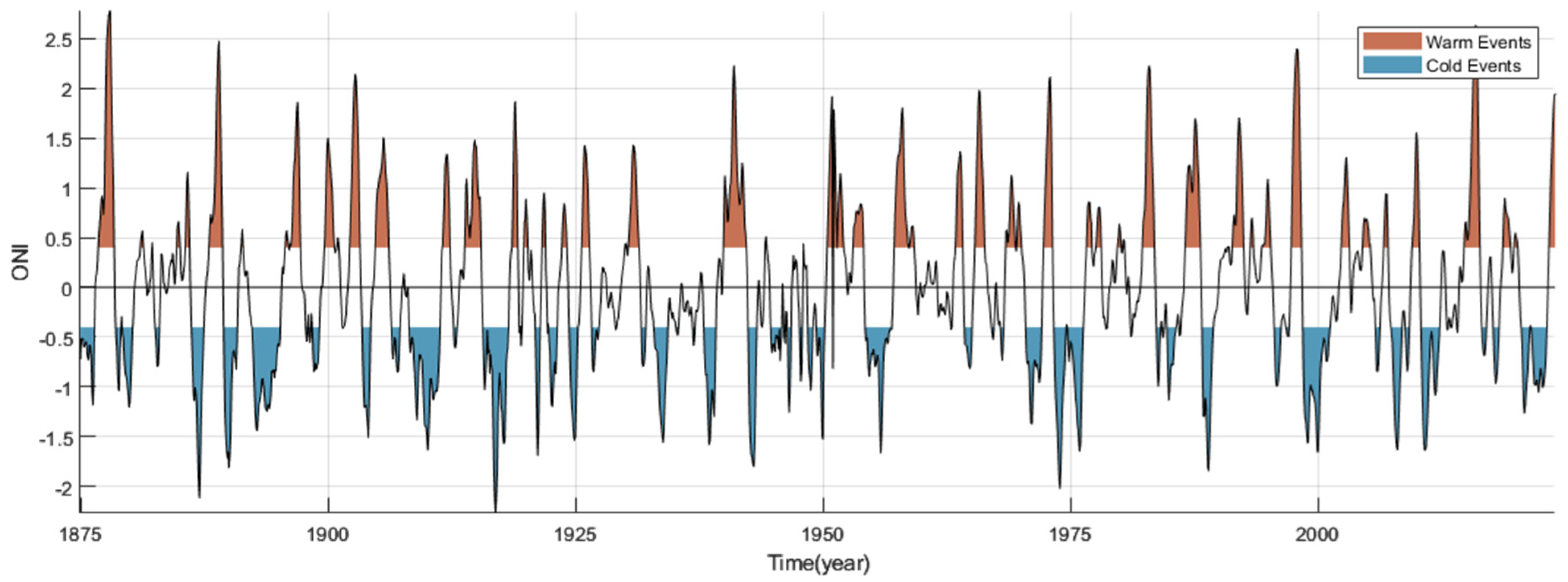
3.1. Definition of ENSO Events

To date, various scholars have used different indicators and datasets, resulting in discrepancies in the criteria for defining ENSO events. Consequently, the establishment and classification of ENSO event intensity exhibit variability, reflecting the continuous evolution of climate standards (see

Table 4. Various ENSO indices and their corresponding standards for defining ENSO events.

Index	Proposer/User	Standards for Identifying ENSO Events
Niño 3	JMA	Niño 3 Index with a 5-Month Moving Average Sustained for 6 Months ≥ 0.5 °C (or ≤−0.5 °C) Constitutes a Warm (Cold) Event
Niño 3.4	Trenberth and Kevin [38]	Niño 3.4 Index with a 5-Month Moving Average Sustained for 6 Months ≥ 0.4 °C (or ≤−0.4 °C) Constitutes a Warm (Cold) Event
Niño Zone SST Anomaly Deviation Values	Li et al. [39]	Niño Composite Area Sea Surface Temperature Anomaly Index ≥ 0.5 °C (or ≤−0.5 °C) Sustained for at Least 6 Months (with One Month Not Meeting the Standard Allowed in Between) is Defined as a Warm (Cold) Event
SOI and Equatorial East Pacific SST Anomalies	Kiladis et al. [40]	SST Anomaly ≥ 0 °C for at Least 3 Seasons and ≥ 0.5 °C for at Least 1 Season, with a Negative SOI and ≤ −1.0, Defines a Warm Event
ONI	CPC	ONI ≥ 0.5 °C (≤−0.5 °C) for 5 Consecutive Months Defines a Warm (Cold) Event

).

This study utilizes the Oceanic Niño Index (ONI) to define ENSO events. The ONI is calculated as the 3-month running mean of SST anomalies in the Niño 3.4 region. Given the significant warming of SST in this area since 1950, using a fixed 30-year climate baseline (such as the 1981–2010 average) to define warm and cold events may not accurately reflect interannual variations in the ENSO. To address this problem, the climate standard value for the ONI is updated every five years, based on multiple 30-year climate averages, allowing for a more accurate reflection of the changing climatic context over time [41]. This dynamic adjustment enhances the representativeness of the ONI, accommodating variations under a warming climate while maintaining consistency and accuracy in the historical definition of ENSO events.

Figure 1 presents the ONI time series from January 1875 to December 2023. Based on data from the CPC, this study identifies 40 warm events and 41 cold events.

3.2. Changes in ENSO Event Intensity

Based on Table 1 and Table 3, the characteristics of extremely strong ENSO events from 1875 to 2023 are summarized in

Table 5. Characteristics of extreme ENSO events from 1875 to 2023.

Event Type	Start Time	End Time	MAX ONI	∑ONI	SST Intensity	MIN/MAX SOI	∑SOI	OAI	Ocean– Atmosphere Intensity	MAX MEI	∑MEI
Warm Events	1876–12	1878–05	2.79	29.16	Extremely strong	−4.34	−28.05	4.23	Extremely strong	2.5	22.97
	1888–02	1889–05	2.48	21.37	Extremely strong	−3.2	−21.3	2.47	Extremely strong	1.89	20.42
	1940–01	1942–03	2.23	30.46	Extremely strong	−3.38	−38.48	5.47	Extremely strong	2.27	36.74
	1982–05	1983–06	2.23	19.91	Extremely strong	−3.46	−29.1	3.07	Extremely strong	2.9	27.6
	1986–09	1988–02	1.7	20.68	Extremely strong	−2.69	−21.89	2.43	Extremely strong	2.1	21.7
	1997–05	1998–04	2.4	21.33	Extremely strong	−3.31	−24.93	2.83	Extremely strong	2.6	25.8
	2015–03	2016–04	2.64	23.65	Extremely strong	−2.61	−20.75	2.73	Extremely strong	2.2	21.7
Cold Events	1892–06	1895–03	−1.44	−33.94	Extremely strong	2.25	19.06	−3.44	Extremely strong	−2.56	−48.64
	1908–04	1911–04	−1.64	−36.92	Extremely strong	2.63	23.1	−4.22	Extremely strong	−2.01	−47.55
	1916–03	1918–03	−2.27	−30.12	Extremely strong	3.48	35.92	−4.84	Extremely strong	−2.17	−35.25
	1954–05	1956–08	−1.67	−22.15	Extremely strong	1.8	22.63	−2.5	Extremely strong	−2.08	−36.48
	1998–07	2001–02	−1.66	−33.54	Extremely strong	2.1	26.59	−4.21	Extremely strong	−1.8	−35.2

, revealing a total of seven extreme warm events and five extreme cold events. Due to the constraints on the length of the main text, we have opted to present only the most intense ENSO events within the main body of this paper. A comprehensive table detailing all ENSO event characteristics during this period has been included in Appendix A (

Table A1. Summary of ENSO event characteristics (warm events) from 1875 to 2023.

Event Type	Start Time	End Time	MAX ONI	∑ONI	SST Intensity	MIN SOI	∑SOI	OAI	Ocean– Atmosphere Intensity	MAX MEI	∑MEI
Warm Events	1876–12	1878–05	2.79	29.16	Extremely strong	−4.34	−28.05	4.23	Extremely strong	2.5	22.97
	1885–09	1886–01	1.16	4.48	Extremely weak	−1.92	−3.65	−1.65	Weak	1.22	3.82
	1888–02	1889–05	2.48	21.37	Extremely strong	−3.2	−21.3	2.47	Extremely strong	1.89	20.42
	1896–05	1897–03	1.86	13.51	Moderate	−3.23	−21.29	1.39	Strong	1.54	12.3
	1899–10	1900–08	1.5	12.04	Moderate	−2.95	−0.6	−0.93	Weak	1.71	13.12
	1902–04	1903–03	2.15	17.79	Strong	−1.76	−1.73	−0.02	Moderate	2.04	16.08
	1904–11	1906–02	1.51	17.56	Strong	−3.51	−24.37	2.26	Extremely strong	1.95	19.25
	1911–09	1912–04	1.34	8.53	Weak	−2.27	−9.61	−0.49	Moderate	1	5.67
	1913–11	1914–04	1.1	4.93	Extremely weak	−2.27	−4.09	−1.54	Weak	0.81	4.34
	1914–06	1915–06	1.48	14	Weak	−2.71	−11.33	0.44	Moderate	1.56	14.34
	1918–09	1919–03	1.87	9.28	Weak	−1.62	−6.83	−0.67	Moderate	1.75	9.05
	1919–11	1920–03	0.89	3.49	Extremely weak	−1.23	−3.09	−1.84	Weak	0.66	2.14
	1923–09	1924–02	0.84	4.25	Extremely weak	−1.46	−4.13	−1.63	Weak	1.02	4.84
	1925–09	1926–05	1.43	9.66	Weak	−1.65	−8.88	−0.41	Moderate	1.71	13.29
	1930–06	1931–05	1.43	12.14	Weak	−1.61	0.36	−1.01	Weak	1.96	19.53
	1940–01	1942–03	2.23	30.46	Extremely strong	−3.38	−38.48	5.47	Extremely strong	2.27	36.74
	1950–07	1950–12	1.92	8.42	Weak	0.63	8.94	−2.4	Extremely weak	−1.03	−8.29
	1951–07	1952–01	1.15	6.11	Extremely weak	−1.44	−7.49	−1.04	Weak	1.23	6.39
	1953–02	1954–01	0.84	8.92	Weak	−2.72	−8.76	−0.52	Moderate	0.78	5.47
	1957–04	1958–07	1.81	18.93	Extremely strong	−1.89	−9.56	0.93	Moderate	1.63	21.24
	1958–11	1959–03	0.62	2.86	Extremely weak	−1.5	−3.12	−1.93	Extremely weak	0.86	3.15
	1963–06	1964–02	1.37	9.4	Weak	−1.46	−6.86	−0.65	Moderate	1.11	7.53
	1965–06	1966–04	1.98	15.29	Strong	−2.32	−14.34	0.92	Moderate	1.73	15.83
	1968–10	1969–05	1.13	6.81	Extremely weak	−1.36	−4.58	−1.24	Weak	1.09	6.86
	1969–08	1970–01	0.86	4.11	Extremely weak	−1.35	−4.36	−1.63	Weak	0.91	4.77
	1972–05	1973–03	2.12	15.35	Strong	−1.84	−12.58	0.75	Moderate	2.21	19.48
	1976–09	1977–02	0.86	4.49	Extremely weak	−1.29	−0.62	−1.96	Extremely weak	1.27	5.29
	1977–09	1978–01	0.81	3.59	Extremely weak	−1.56	−5.61	−1.57	Weak	1.11	4.61
	1982–05	1983–06	2.23	19.91	Extremely strong	−3.46	−29.1	3.07	Extremely strong	2.9	27.6
	1986–09	1988–02	1.7	20.68	Extremely strong	−2.69	−21.89	2.43	Extremely strong	2.1	21.7
	1991–06	1992–06	1.71	14.06	Moderate	−2.85	−18.48	1.18	Strong	2	16.2
	1994–09	1995–03	1.09	5.6	Extremely weak	−1.7	−6.12	−1.25	Weak	1.5	6
	1997–05	1998–04	2.4	21.33	Extremely strong	−3.31	−24.93	2.83	Extremely strong	2.6	25.8
	2002–06	2003–02	1.31	8.52	Weak	−1.62	−7.89	−0.66	Moderate	1	6.5
	2004–08	2005–02	0.7	4.58	Extremely weak	−2.99	−6.42	−1.35	Weak	0.8	3.6
	2006–09	2007–01	0.94	3.85	Extremely weak	−1.52	−3.29	−1.77	Weak	1	3.7
	2009–08	2010–03	1.56	8.78	Weak	−1.66	−7.64	−0.65	Moderate	1.3	7.1
	2015–03	2016–04	2.64	23.65	Extremely strong	−2.61	−20.75	2.73	Extremely strong	2.2	21.7
	2018–10	2019–05	0.9	5.85	Weak	−1.43	−2.12	−1.62	Weak	0.8	2.9
	2023–06	2023–12	1.95	10.37	Extremely weak	−1.6	−5.35	−0.67	Moderate	1.1	4.6

and

Table A2. Summary of ENSO event characteristics (cold events) from 1875 to 2023.

Event Type	Start Time	End Time	MIN ONI	∑ONI	SST Intensity	MAX SOI	∑SOI	OAI	Ocean– Atmosphere Intensity	MAX MEI	∑MEI
Cold Events	1875–01	1876–05	−1.19	−11.77	Weak	2.57	6.97	0.36	Moderate	−1.96	−20.54
	1878–09	1879–01	−1.04	−4.27	Extremely weak	1.89	7.2	1.18	Weak	−1	−4.05
	1879–05	1880–03	−1.21	−10.14	Weak	2.2	12.99	−0.11	Moderate	−1.18	−9.19
	1886–04	1887–06	−2.12	−18.48	Strong	1.51	12.48	−0.99	Moderate	−1.57	−17.46
	1889–07	1890–11	−1.82	−19.46	Strong	2.35	12.57	−1.11	Strong	−1.73	−22.91
	1892–06	1895–03	−1.44	−33.94	Extremely strong	2.25	19.06	−3.44	Extremely strong	−2.56	−48.64
	1898–07	1899–02	−0.85	−6.11	Extremely weak	1.31	5.21	1.19	Weak	−1.09	−4.79
	1903–07	1904–04	−1.52	−11.44	Weak	3.64	10.62	0	Moderate	−1.25	−8.28
	1906–07	1907–04	−0.86	−6.71	Extremely weak	1.95	6.09	1.03	Weak	−1.18	−7.41
	1908–04	1911–04	−1.64	−36.92	Extremely strong	2.63	23.1	−4.22	Extremely strong	−2.01	−47.55
	1915–09	1916–01	−1.03	−4.01	Extremely weak	1.34	2.1	1.76	Weak	−0.69	−1.79
	1916–03	1918–03	−2.27	−30.12	Extremely strong	3.48	35.92	−4.84	Extremely strong	−2.17	−35.25
	1921–01	1921–05	−1.7	−6.13	Extremely weak	1.09	1.45	1.59	Weak	−1.12	−2.61
	1922–05	1923–02	−1.2	−8.59	Weak	1.21	3.52	1.09	Weak	−0.84	−4.58
	1924–06	1925–03	−1.54	−11.86	Weak	1.52	8.65	0.17	Moderate	−1.46	−10.27
	1926–09	1927–01	−0.85	−3.43	Extremely weak	0.59	1.53	1.89	Weak	−0.03	0.14
	1933–01	1934–04	−1.56	−16.41	Moderate	0.81	2.21	0.36	Moderate	−1.25	−11.95
	1938–01	1939–03	−1.59	−16.18	Moderate	2.01	14.05	−0.9	Moderate	−1.39	−12.37
	1942–07	1943–04	−1.8	−14.32	Moderate	1.59	6.19	0.16	Moderate	−1.26	−9.45
	1944–10	1945–03	−0.66	−3.64	Extremely weak	1.33	0.78	1.95	Extremely weak	−0.47	−2.23
	1946–06	1946–10	−1.26	−4.61	Extremely weak	−0.64	−5.91	2.56	Extremely weak	−0.19	0.19
	1948–07	1948–12	−1.04	−4.85	Extremely weak	0.54	−1.2	2.03	Extremely weak	−0.28	−0.54
	1949–06	1950–02	−1.53	−8.05	Weak	1.58	0.28	1.51	Weak	−1.13	−6.5
	1954–05	1956–08	−1.67	−22.15	Extremely strong	1.8	22.63	−2.5	Extremely strong	−2.08	−36.48
	1964–05	1965–01	−0.82	−6.17	Extremely weak	1.32	4.12	1.3	Weak	−1.29	−9.46
	1970–07	1972–01	−1.38	−16.9	Moderate	2.58	18.59	−1.48	Strong	−1.98	−24.79
	1973–05	1974–07	−2.03	−18.8	Moderate	2.85	19.64	−1.8	Strong	−2.19	−20.71
	1974–10	1976–03	−1.65	−18.09	Strong	2.15	19.8	−1.74	Strong	−2.27	−24.38
	1984–10	1985–06	−1.14	−7.47	Extremely weak	1.42	−0.41	1.65	Weak	−1.2	−5.2
	1988–05	1989–05	−1.85	−16.52	Strong	2.18	16.03	−1.16	Strong	−1.8	−17.3
	1995–08	1996–03	−1	−6.54	Extremely weak	0.82	0.42	1.66	Weak	−0.9	−6.3
	1998–07	2001–02	−1.66	−33.54	Extremely strong	2.1	26.59	−4.21	Extremely strong	−1.8	−35.2
	2005–11	2006–03	−0.85	−3.6	Extremely weak	1.32	2.08	1.81	Weak	−0.7	−3.1
	2007–07	2008–06	−1.64	−13.79	Moderate	2.05	7.72	0.05	Moderate	−1.5	−12.9
	2008–11	2009–03	−0.85	−3.53	Extremely weak	1.64	5.08	1.49	Weak	−1	−4.7
	2010–06	2011–05	−1.64	−14.31	Moderate	3.02	22.42	−1.6	Strong	−2.4	−22.5
	2011–08	2012–03	−1.09	−6.76	Extremely weak	2.45	7.3	0.89	Moderate	−1.3	−7.9
	2016–08	2016–12	−0.69	−3.09	Extremely weak	1.28	0.98	1.99	Extremely weak	−0.5	−2
	2017–10	2018–04	−0.97	−5.43	Extremely weak	1.03	3.21	1.48	Weak	−1.3	−5.5
	2020–08	2021–04	−1.27	−8.57	Weak	1.76	7.47	0.67	Moderate	−1.2	−9.4
	2021–09	2023–01	−1.06	−15.38	Moderate	2.69	22.15	−1.69	Strong	−2.2	−25.1

). All abbreviations and their descriptions used in the article are shown in

Table A3. List of abbreviations used in this article.

Abbreviation	Full Term	Description
ENSO	El Niño–Southern Oscillation	A climate phenomenon involving periodic changes in Pacific sea surface temperature and atmospheric pressure.
SO	Southern Oscillation	Atmospheric pressure variations in the Pacific associated with the ENSO.
SLP	Sea Level Pressure	The atmospheric pressure measured at sea level.
SST	Sea Surface Temperature	The temperature of the ocean’s surface layer.
SSTA	Sea Surface Temperature Anomaly	Deviation of sea surface temperature from its average.
SOI	Southern Oscillation Index	An index measuring pressure differences between Darwin and Tahiti, indicating SO strength.
MEI	Multivariate ENSO Index	An index that combines multiple climate variables to describe ENSO strength.
ONI	Oceanic Niño Index	An index based on sea surface temperature anomalies in the Pacific to identify ENSO events.
OAI	Ocean–Atmosphere Intensity Index	An index quantifying the interaction between the ocean and atmosphere.
WPS	Wavelet Power Spectrum	A representation of signal energy across different frequency scales.
GWS	Global Wavelet Spectrum	The total power distribution of a signal across various scales.
XWT	Cross-Wavelet Transform	A method to analyze phase relationships and shared frequencies between two signals.
WTC	Wavelet Transform Coherence	A measure of the coherence between two signals across different scales.
CPC	Climate Prediction Center	A U.S. agency focused on climate prediction and monitoring.
JMA	Japan Meteorological Agency	Japan’s national agency responsible for weather forecasting and research.
MAM	March–April–May	A period from March to May, representing spring in the Northern Hemisphere.
JJA	June–July–August	A period from June to August, representing summer in the Northern Hemisphere.
SON	September–October–November	A period from September to November, representing autumn in the Northern Hemisphere.
DJF	December–January–February	A period from December to February, representing winter in the Northern Hemisphere.

.Among all ENSO events, there is a predominance of weak and very weak events, constituting 62.5% (25 events) of warm events and 58.5% (24 events) of cold events. Notably, 80% of ENSO events lasting 5 months are classified as very weak. Many scholars define the duration of ENSO events as lasting more than 6 months [42,43], which typically excludes very weak events from their ENSO event tables. Although the onset and duration of events may vary due to differing definitions and metrics, the overall trends observed in this study align closely with the existing literature.

Different indices reflect various aspects of the ENSO, leading to discrepancies in the assessment of event intensity. For instance, the ONI cumulative value indicates that the strongest warm event occurred in 2015/2016; however, the SOI and the OAI suggest that the most intense warm event took place in 1982/1983. In contrast, the MEI indicates that the warm event of 1997/1998 was the strongest based on its extreme values and cumulative totals. Given the multifaceted impacts of the ENSO on oceanic and atmospheric systems, it remains challenging to derive a singular comprehensive index that accurately represents all aspects of the ENSO. Currently, the MEI includes only six primary variables. The ENSO is a complex, dynamic system, making it appropriate to employ multiple characteristics for its assessment.

To better investigate the characteristics of ENSO intensity changes, Figure 2 represents the strength of warm events using the following scale: extreme (5), strong (4), moderate (3), weak (2), and very weak (1). For cold events, the scale is as follows: extreme (−5), strong (−4), moderate (−3), weak (−2), and very weak (−1), with (0) indicating normal years. A moving trend fit is applied to analyze ENSO intensity.

The results reveal significant fluctuations in ENSO intensity over the past 150 years. Notably, the period from the 1870s to the 1910s exhibits considerable volatility, while fluctuations between the 1920s and 1960s are relatively stable. Beginning in the 1970s, the variability increases again, alongside a rise in the frequency of extreme warm events.

The statistics on the starting seasons of ENSO events from 1875 to 2023 (Figure 3a) indicate that warm events mainly occur in JJA and SON, while cold events predominantly take place in JJA. Notably, extreme cold events such as those in 1892/1895, 1954/1956, and 1998/2001 occurred during JJA. Although the number of warm events in MAM is lower than in JJA and SON, these MAM warm events are often classified as strong or extreme. In SON, with the exception of the strong warm event in 1986/1988, the remaining events were weak or very weak cold events. The occurrence of warm and cold events in DJF is similar, including three extreme warm events, while the cold events generally exhibit lower intensity. The statistics on ONI peak months (Figure 3b) reveal that the peaks of ENSO events predominantly occur in SON and DJF, with a higher frequency in DJF.

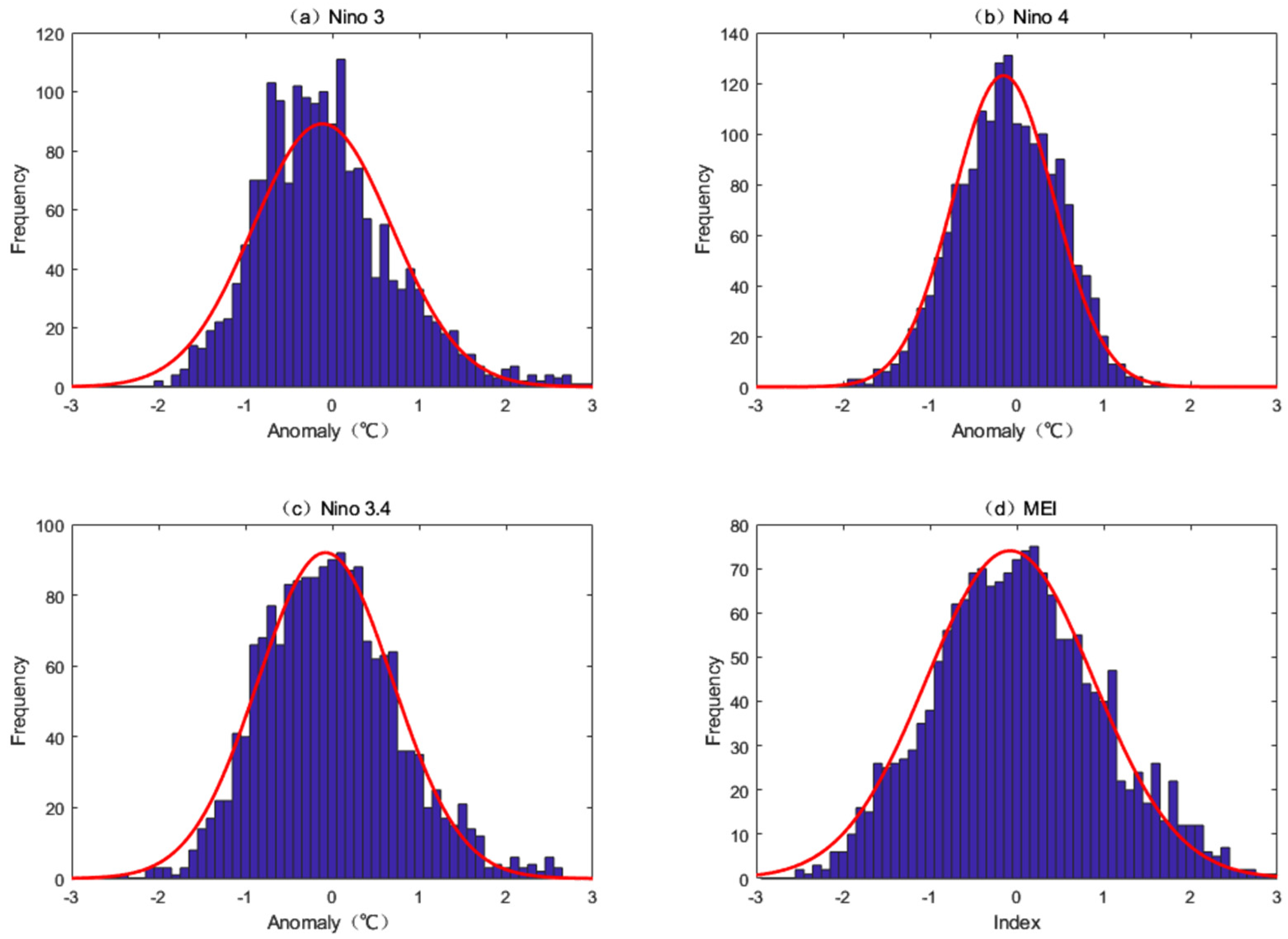
3.3. Frequency Distribution of ENSO Events

From January 1875 to December 2023, out of 1788 months, there were 406 months classified as warm events, accounting for 22.7%; 522 months as cold events, making up 29.2%; and the remaining 386 months represented normal conditions, comprising 48.1%. This finding indicates that ENSO events were present for 51.9% of the time. The frequency distribution of ENSO events is illustrated in Figure 4, where the 0 value on the x-axis can be approximated as the average over the entire period.

Calculations show that the Niño3, Niño4, and Niño3.4 indices and the MEI do not strictly adhere to a standard normal distribution (

Table 6. Standard kurtosis (K) and skewness (SK) coefficients of the four indices (kurtosis coefficient = 3, skewness coefficient = 0 for standard normal distribution).

Index	Niño3	Niño4	Niño3.4	MEI
K	4.1888	2.7525	3.3886	2.7116
SK	0.788	−0.1166	0.4376	0.2326

). The Niño3 index exhibits a high kurtosis, as evident in Figure 4a, where there are many data points near the mean. A distribution with positive excess kurtosis has heavier tails, indicating that it contains more data in the extremes compared to a normal distribution. The Niño3 index also has a positive skewness, resulting in a pronounced tail in the positive region. Conversely, the Niño4 index exhibits characteristics opposite to those of the Niño3 index, with fewer data points near the mean than expected in a normal distribution. This finding suggests a platykurtic distribution with negative skewness and a tail in the negative region, indicating that the Niño4 index is more suited for representing cold events (Figure 4b).

The Niño3.4 index and the MEI effectively reflect ENSO events, with similar kurtosis and skewness coefficients for both. Figure 4c,d demonstrates sharp peak and heavy tail characteristics, where the positive and negative anomaly regions are nearly symmetrical. The positive anomaly region has segments that exceed the normal distribution curve in the tail, while parts of the negative anomaly region also lie above the normal distribution curve. This finding explains why the occurrence counts for warm and cold events are roughly consistent in Table 5. The positive skew and heavy tail frequency distribution of the Niño3.4 and MEI curves provide a basis for determining the anomalies in sea surface temperature in the Central-Eastern equatorial Pacific, indicating that the proportion of months with strong warm events is greater than that for strong cold events throughout the entire period.

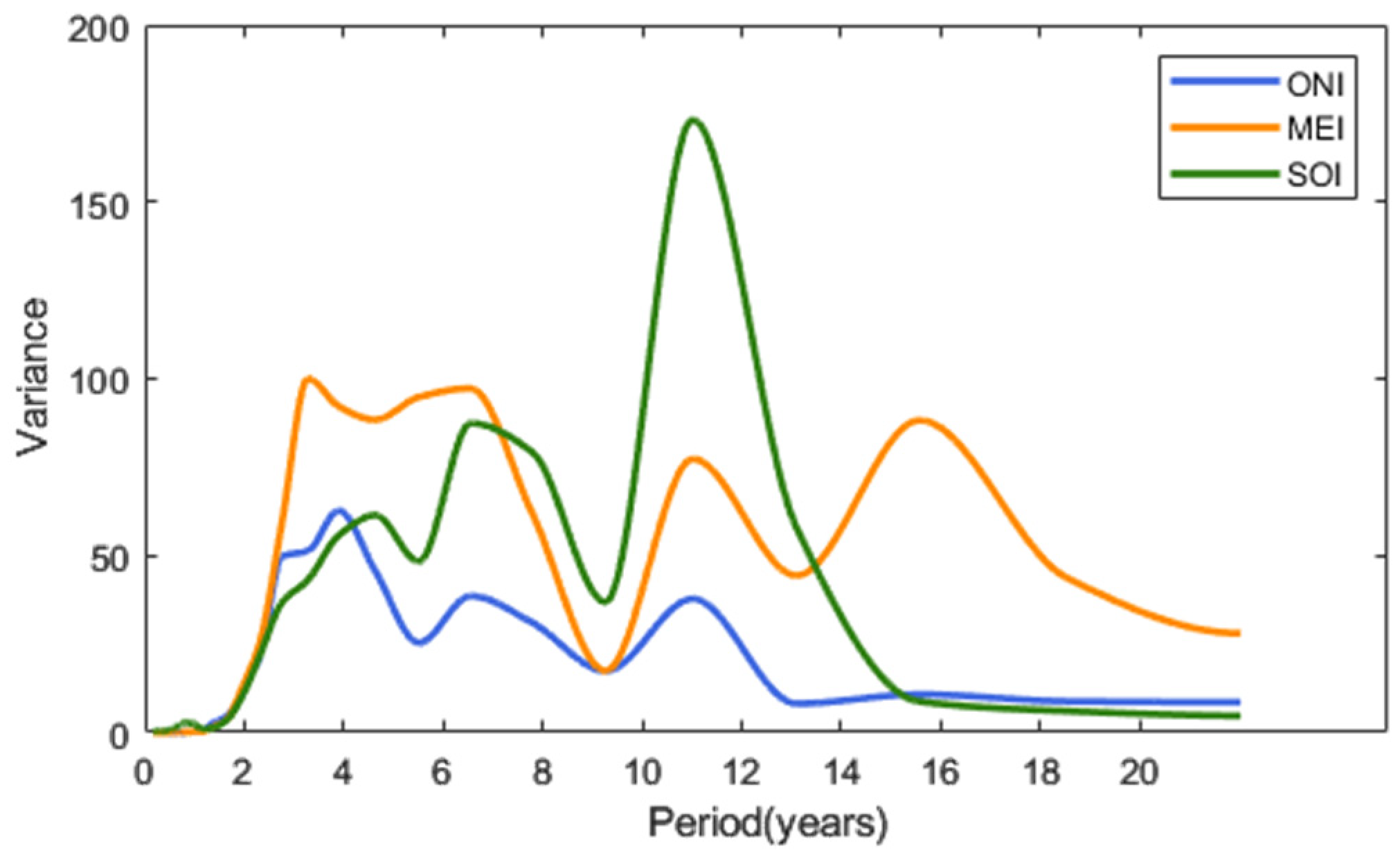
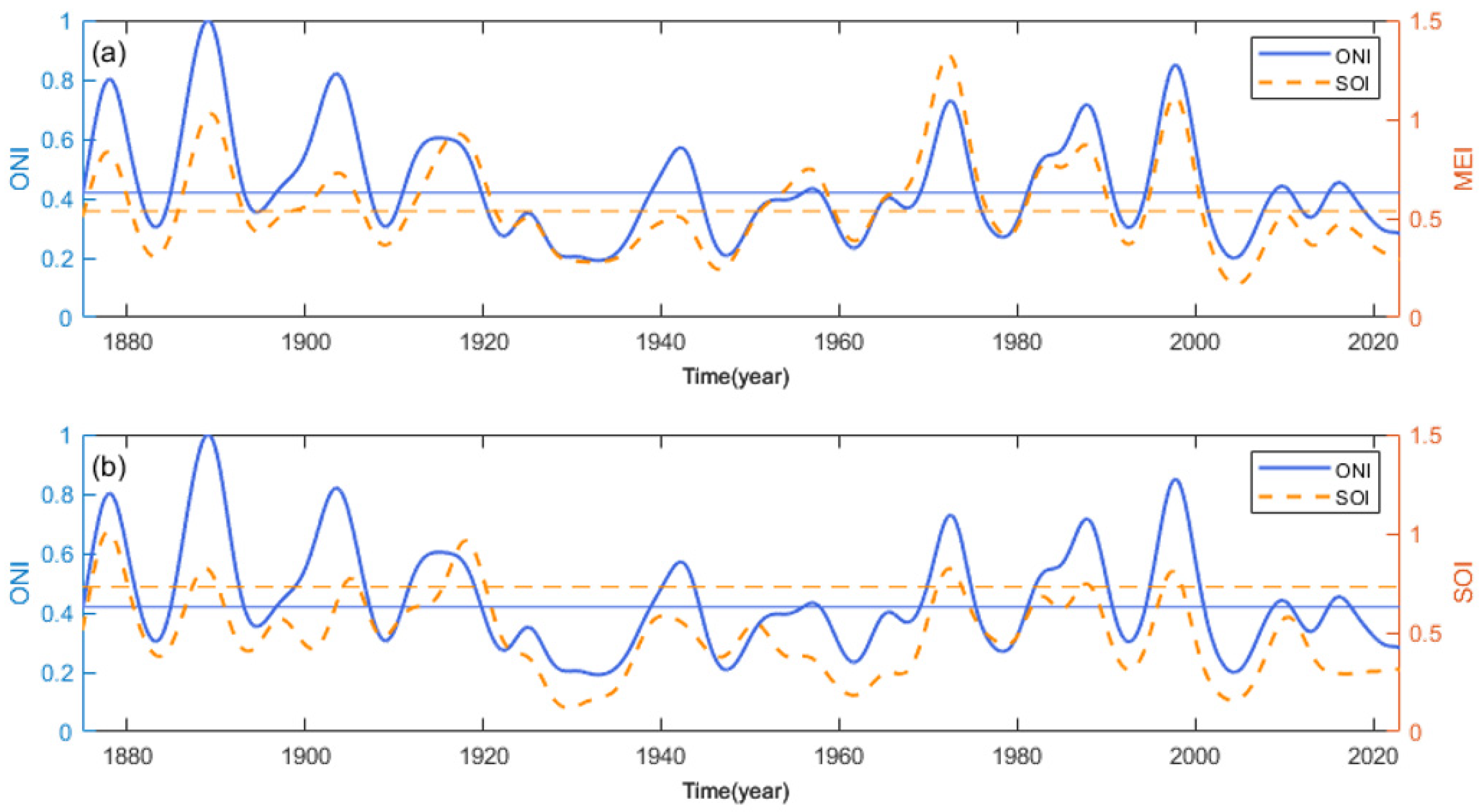
3.4. Interannual and Decadal Oscillations of ENSO Events

To better investigate the variation characteristics of ENSO signals across different timescales, this study conducts a Morlet wavelet analysis on three key indices representing the ENSO: the ONI, SOI, and MEI (Figure 5). The results indicate that the time–frequency characteristics of the ONI and MEI indices are similar, exhibiting strong consistency. Both indices show significant wavelet power spectra in the 2–8-year periodic band, corresponding to the interannual oscillation of the ENSO, with another high-value band located in the 8–16-year range, representing decadal changes in ENSO. The wavelet power spectrum of the SOI also demonstrates oscillations in the 2–7-year range, although the area of significance is smaller compared to the ONI and MEI.

In the wavelet global spectrum, the significant periods for the ONI range from 2 to 6 years, while, for the MEI, it is 2–5 years. Notably, both indices exhibit a bimodal structure in their significant periods, with peaks at 3 and 5 years. The significant periods in the wavelet global spectrum for the SOI are found at 2–4 years, 5–8 years, and 10–14 years, with a peak around 12 years. The fluctuations of the wavelet global spectrum for the ONI and the SOI are similar in the 4–16-year range.

In the wavelet real part (Figure 5b,d,f), the positive center of the ONI and MEI corresponds to warm events, while the negative center aligns with cold events; the opposite is true for the SOI. Combining the 95% significance regions from the wavelet power spectrum with the wavelet real part, it is observed that the primary periodicity of ENSO cycles in the 1950s was mainly in the 4–8-year range. Starting from the 1960s, the periodicity of ENSO modes shortened, and the amplitude continually increased, with the entire wave pattern shifting towards lower frequencies. Between 1960 and 2000, the primary significant period of ENSO cycles was 2–7 years, while the power spectrum of the SOI indicated significant decadal oscillations in the atmosphere at 10–15 years. Beginning in 2000, the main period of ENSO cycles further shortened to 2–4 years, validated by a 5% significance level.

Figure 6 presents the wavelet variance of the ONI, SOI, and MEI, illustrating that their trends are closely aligned. The wavelet variance of the ONI shows high-value regions at 3–5 years and 10–13 years, while the SOI has high-value areas at 3–8 years and 10–13 years. The MEI exhibits high values in the 3–8-year and 10–17-year ranges. Additionally, the dominant periodicity of the ENSO is observed at 3–5 years. Furthermore, both the MEI and SOI display high variance in periods exceeding 32 years; however, this region lies outside the influence cone in the power spectrum and is therefore excluded from consideration.

Based on the above analysis, this study defines the 3–8 year scale as the primary mode of the ENSO from 1875 to 2023, with the 10–16 year scale representing decadal changes in ENSO, followed by further discussion. To investigate the wavelet energy fluctuations and interannual and decadal oscillations associated with the ENSO mode, the average wavelet energy can be derived from the wavelet power spectrum’s weights at the 3–8 year scale. This average wavelet energy reflects the mean variance of the time series within this band, allowing for the observation of changes in the average variance of the ENSO mode over time. The 3–8 year wavelet average variance series for the ONI, SOI, and MEI demonstrates strong consistency (Figure 7).

The wavelet energy series for the 3–8 year scale of the ENSO has shown significant variability over the past 150 years, maintaining a high energy level from 1875 to 1920, followed by a decrease from 1920 to 1961. Energy levels began to increase in the 1960s, with a marked high variance period for the ENSO from 1961 to 2000, while a lower energy level was observed from 2001 to 2023. These four periods can be defined as distinct decadal variations in the wavelet variance of the ENSO mode from 1875 to 2023.

The 3–8 year scale has shown significant energy levels at the 5% significance level for the periods of 1875–1881, 1885–1892, 1913–1920, 1940–1945, 1970–1975, 1982–1989, and 1995–1999, corresponding to strong warm and cold events (as indicated in Table 5). Key peaks in the energy spectrum are found in the years 1877, 1888, 1905, 1916, 1942, 1957, 1965, 1972, 1983, 1988, 1998, 2009, and 2016, with 1905, 1965, and 2009 representing moderate or strong warm events, while the remaining years correspond to extreme warm events. Notable troughs in the energy spectrum occur in 1884, 1894, 1909, 1922, 1930, 1948, 1961, 1967, 1978, 1993, 2004, and 2013, which correspond to weak or extremely weak warm or cold events, or periods without ENSO events. This finding indicates that stronger interannual oscillations are associated with greater intensity of ENSO events.

Based on the continuous wavelet transform, cross wavelet transform, and wavelet coherence analysis, it is possible to reveal areas where two sequences share common signals and their phase relationships, which is beneficial for further investigating the correlations and consistencies among ENSO characteristic values [44]. The cross wavelet transform emphasizes the interrelationships in high-energy regions of the time–frequency domain, while wavelet coherence highlights relationships in low-energy regions [45].

As shown in Figure 8, the cross wavelet spectra reveal that the common signals of the ONI, MEI, and SOI are evident in the 5% significance level regions depicted in Figure 8a,c,e. This finding indicates that the ONI, MEI, and SOI exhibit strong energy resonance at the 3–8 year scale, highlighting the ENSO signal. Throughout the entire time span, the ONI and MEI show a phase relationship that is out-of-phase with the SOI in their significant high-energy regions, whereas the ONI and MEI are in-phase with each other, confirming that these three indices largely reflect one another. Moreover, the phase relationships outside the significant regions are primarily either out-of-phase or in-phase.

Thus, it can be inferred that the connections among the ONI, MEI, and SOI are stronger than what is represented in the cross wavelet power spectrum. Figure 8b,d,f presents the wavelet coherence spectra for the three ENSO characteristic values, which show larger significant regions that span almost all time scales, with all areas displaying either in-phase relationships (the ONI with the MEI) or out-of-phase relationships (the ONI with SOI and the MEI with the SOI). The lower energy region in the wavelet coherence spectrum of the ONI and the SOI (Figure 8d) aligns with the low-value area of the wavelet power spectrum in Figure 5a.

Through cross wavelet transformation and wavelet coherence analysis, a deeper correlation among ENSO characteristic values can be established, rather than merely describing their close relationships using correlation coefficients. The high correlation and consistency among the three ENSO characteristic values render their results reliable for characterizing the ENSO. Therefore, it is concluded that the ENSO exhibits interannual oscillations at the 3–8 year scale from 1875 to 2023.

4. Discussion and Conclusions

This study addresses the complexities involved in quantifying ENSO variability and offers a robust framework for understanding its implications over the nearly 150-year period from January 1875 to December 2023. We defined ENSO events using the ONI, establishing that a value of ≥0.5 °C for warm events and ≤−0.5 °C for cold events sustained for five consecutive months serves as the foundational criterion for classification. This approach allowed us to identify a total of 40 warm events and 41 cold events, highlighting the variability and dynamism of ENSO phenomena. The analysis further categorized ENSO event intensities by examining sea surface temperature and ocean–atmosphere intensity indices.

Since the impact of ENSO events is characterized by ocean–atmosphere coupling, the ENSO event intensity evaluation metric used in this study, which comprehensively considers both SST and ocean–atmosphere interaction strength, provides a more convincing assessment. Research conducted by Quinn et al. [10] only considered the impact of SST, which led to a bias in determining the overall strength of the 1957 warm event, where SST intensity was extremely strong, but ocean–atmosphere interaction strength was moderate. A study conducted by Feng et al. [16], based on principal component analysis and remote correlation with precipitation anomalies, cannot explain the relationship between ENSO event intensity and precipitation anomalies from a mechanistic perspective, and precipitation data from a single location are not representative. Kido et al. [20] used climate models to simulate ENSO events and defined and predicted ENSO event intensity through coupling with global precipitation anomalies. This is a novel approach that provides new ideas for future research. In our future studies, we will consider coupling SST, ocean–atmosphere interaction intensity, and global precipitation anomalies to define and predict ENSO event intensity.

We identified seven extreme warm events and five extreme cold events, with all MAM occurrences of El Niño classified as strong or extreme. Notably, the results indicate that ENSOs’ peak intensity tends to align with DJF, emphasizing seasonal trends in event occurrence. This result aligns with the findings of Capotondi et al. [5], which demonstrate that the seasonal variation and development of ENSO events exhibit clear and distinct characteristics.

We also discussed the historical variations in the frequency and intensity of ENSO events. From the 1870s to the 1950s, ENSO events were less frequent and weaker, with limited and inconsistent observational data. These events were typically mild and short-lived [34,43]. In the 1950s−1980s, as early signs of climate change appeared, ENSO events became more intense, with notable episodes in the 1960s and 1970s (e.g., 1972–1973 and 1982–1983 El Niño events) [5]. Research suggests an increase in ENSO intensity, especially with stronger and more frequent El Niño occurrences [42]. From the 1990s to 2023, ENSO events became more frequent and intense. The 1997–1998 and 2015–2016 El Niño events were particularly strong, causing widespread extreme weather. Studies indicate an upward trend in ENSO intensity in the 21st century [15,46].

A key finding of this research is the positive skewness and heavy-tailed distribution of ENSO characteristic values, indicating that stronger warm events occur more frequently than strong cold events. This asymmetry highlights the unique impact of the ENSO on the global climate, reinforcing the notion that understanding these dynamics is essential for predicting future climate patterns. The primary oscillation modes of the ENSO were determined to be interannual scales of 3 to 8 years, alongside a decadal oscillation range of 10 to 16 years.

The interannual and decadal variations in the ENSO have also been demonstrated in studies conducted by Guilyardi et al. [46] and Dieppois et al. [15] Furthermore, research conducted by Delage and Power [47] identified an interannual variability period of 4–7 years for the ENSO, which is attributable to their consideration of global precipitation anomalies. Studies conducted by Geng et al. [48] using climate models to simulate future climate change under greenhouse gas forcing indicate that the frequency of consecutive La Niña events and extreme ENSO events may increase. This research also provides new insights for our future research, where we plan to incorporate climate variables corresponding to the relevant timescales into the study of interannual and decadal variations to enhance our understanding of ENSO variability.

In conclusion, this research significantly enhances our understanding of ENSO dynamics and provides a reliable framework for event intensity patterns based on the sea surface temperature intensity and ocean–atmosphere intensity. The findings reveal critical insights into the frequency and intensity of ENSO events over the past century and a half, contributing to a broader understanding of climate variability and its implications for global climate systems.

References

1. Neelin, J.D.; Battisti, D.S.; Hirst, A.C.; Jin, F.F.; Wakata, Y.; Yamagata, T.; Zebiak, S.E. ENSO theory. J. Geophys. Res. Ocean. 1998, 103, 14261–14290. [Google Scholar] [CrossRef]
2. Wang, C. A review of ENSO theories. Natl. Sci. Rev. 2018, 5, 813–825. [Google Scholar] [CrossRef]
3. Tang, Y.; Zhang, R.-H.; Liu, T.; Duan, W.; Yang, D.; Zheng, F.; Ren, H.; Lian, T.; Gao, C. Progress in ENSO prediction and predictability study. Natl. Sci. Rev. 2018, 5, 826–839. [Google Scholar] [CrossRef]
4. McPhaden, M.J.; Zebiak, S.E.; Glantz, M.H. ENSO as an integrating concept in earth science. Science 2006, 314, 1740–1745. [Google Scholar] [CrossRef]
5. Capotondi, A.; Wittenberg, A.T.; Kug, J.S.; Takahashi, K.; McPhaden, M.J. ENSO diversity. El Niño South. Oscil. A Chang. Clim. 2020, 65–86. [Google Scholar]
6. Bjerknes, J. Atmospheric teleconnections from the equatorial Pacific. Mon. Weather Rev. 1969, 97, 163–172. [Google Scholar] [CrossRef]
7. Rasmusson, E.M.; Wallace, J.M. Meteorological aspects of the El Nino/southern oscillation. Science 1983, 222, 1195–1202. [Google Scholar] [CrossRef]
8. Philander, S.G.H. El Nino southern oscillation phenomena. Nature 1983, 302, 295–301. [Google Scholar] [CrossRef]
9. Richard, Y.; Trzaska, S.; Roucou, P.; Rouault, M. Modification of the southern African rainfall variability/ENSO relationship since the late 1960s. Clim. Dyn. 2000, 16, 883–895. [Google Scholar] [CrossRef]
10. Quinn, W.H.; Zopf, D.O.; Short, K.S.; Yang, R.K. Historical trends and statistics of the Southern Oscillation, El Niño, and Indonesian droughts. Fish. Bull. 1978, 76, 663–678. [Google Scholar]
11. Wolter, K.; Timlin, M.S. Measuring the strength of ENSO events: How does 1997/98 rank? Weather 1998, 53, 315–324. [Google Scholar] [CrossRef]
12. Wang, S.; Gong, D. ENSO events and their intensity during the past century. Meteorol. Mon. 1999, 25, 9–14. [Google Scholar]
13. Li, X.; Zhai, P. On Indices and Indicators of Enso Episodes. Acta Meteorol. Sin. 2000, 1, 102–109. [Google Scholar]
14. Tedeschi, R.G.; Sampaio, G. Influences of different intensities of El Niño–Southern Oscillation on South American precipitation. Int. J. Climatol. 2022, 42, 7987–8007. [Google Scholar] [CrossRef]
15. Dieppois, B.; Capotondi, A.; Pohl, B.; Chun, K.P.; Monerie, P.-A.; Eden, J. ENSO diversity shows robust decadal variations that must be captured for accurate future projections. Commun. Earth Environ. 2021, 2, 212. [Google Scholar] [CrossRef]
16. Feng, Y.; Chen, X.; Tung, K.-K. ENSO diversity and the recent appearance of Central Pacific ENSO. Clim. Dyn. 2020, 54, 413–433. [Google Scholar] [CrossRef]
17. Emmanuel, I. Linkages between El Niño-Southern Oscillation (ENSO) and precipitation in west Africa regions. Arab. J. Geosci. 2022, 15, 675. [Google Scholar] [CrossRef]
18. Zhou, W.; Wang, X. Wavelet Multiview-Based Hybrid Deep Learning Model for Forecasting El Niño-Southern Oscillation Cycles. Atmos. Clim. Sci. 2024, 14, 450–473. [Google Scholar]
19. Cerón, W.L.; Kayano, M.T.; Andreoli, R.V.; Canchala, T.; Carvajal-Escobar, Y.; Alfonso-Morales, W. Rainfall variability in southwestern Colombia: Changes in ENSO-related features. Pure Appl. Geophys. 2021, 178, 1087–1103. [Google Scholar] [CrossRef]
20. Kido, S.; Richter, I.; Tozuka, T.; Chang, P. Understanding the interplay between ENSO and related tropical SST variability using linear inverse models. Clim. Dyn. 2023, 61, 1029–1048. [Google Scholar] [CrossRef]
21. Wang, B. Interdecadal changes in El Nino onset in the last four decades. J. Clim. 1995, 8, 267–285. [Google Scholar] [CrossRef]
22. Wang, B. Transition from a cold to a warm state of the El Niño-Southern Oscillation cycle. Meteorol. Atmos. Phys. 1995, 56, 17–32. [Google Scholar] [CrossRef]
23. Kirtman, B.P.; Schopf, P.S. Decadal variability in ENSO predictability and prediction. J. Clim. 1998, 11, 2804–2822. [Google Scholar] [CrossRef]
24. Wang, B.; Wang, Y. Temporal structure of the Southern Oscillation as revealed by waveform and wavelet analysis. J. Clim. 1996, 9, 1586–1598. [Google Scholar] [CrossRef]
25. Torrence, C.; Webster, P.J. The annual cycle of persistence in the El Nño/Southern Oscillation. Q. J. R. Meteorol. Soc. 1998, 124, 1985–2004. [Google Scholar] [CrossRef]
26. Torrence, C.; Webster, P.J. Interdecadal changes in the ENSO–monsoon system. J. Clim. 1999, 12, 2679–2690. [Google Scholar] [CrossRef]
27. Torrence, C.; Compo, G.P. Wavelet analysis. Bull. Am. Meteorol. Soc. 2004, 79, 61–78. [Google Scholar] [CrossRef]
28. Zhang, Q.; Ding, Y. Decadal Climate Change and Enso Cycle. Acta Meteorol. Sin. 2013, 59, 157–172. [Google Scholar]
29. QIN, J.; WANG, Y. Construction of new indices for the two types of ENSO events. Acta Meteorol. Sin. 2014, 72, 526–541. [Google Scholar]
30. Schneider, D.P.; Deser, C.; Fasullo, J.; Trenberth, K.E. Climate data guide spurs discovery and understanding. Eos Trans. Am. Geophys. Union 2013, 94, 121–122. [Google Scholar] [CrossRef]
31. Wolter, K.; Timlin, M.S. Monitoring ENSO in COADS with a seasonally adjusted principal. In Proceedings of the 17th Climate Diagnostics Workshop, Norman, OK, USA, 18–23 October 1992; NOAA/NMC/CAC; NSSL; Oklahoma Climate Survey. CIMMS and the School of Meteorology, University of Oklahoma: Norman, OK, USA, 1992. [Google Scholar]
32. Wolter, K.; Timlin, M.S. El Niño/Southern Oscillation behaviour since 1871 as diagnosed in an extended multivariate ENSO index (MEI. ext). Int. J. Climatol. 2011, 31, 1074–1087. [Google Scholar] [CrossRef]
33. Hanley, D.E.; Bourassa, M.A.; O’Brien, J.J.; Smith, S.R.; Spade, E.R. A quantitative evaluation of ENSO indices. J. Clim. 2003, 16, 1249–1258. [Google Scholar] [CrossRef]
34. Wang, C.; Deser, C.; Yu, J.-Y.; DiNezio, P.; Clement, A. El Niño and southern oscillation (ENSO): A review. In Coral Reefs of the Eastern Tropical Pacific. Persistence Loss A Dynamic Environment; Springer: Dordrecht, The Netherlands, 2017; pp. 85–106. [Google Scholar]
35. Falayi, E.; Adewole, A.; Adelaja, A.; Ogundile, O.; Roy-Layinde, T.J.N.J.o.A. Study of nonlinear time series and wavelet power spectrum analysis using solar wind parameters and geomagnetic indices. NRIAG J. Astron. Geophys. 2020, 9, 226–237. [Google Scholar] [CrossRef]
36. Auchère, F.; Froment, C.; Bocchialini, K.; Buchlin, E.; Solomon, J. On the Fourier and wavelet analysis of coronal time series. Astrophys. J. 2016, 825, 110. [Google Scholar] [CrossRef]
37. Grinsted, A.; Moore, J.C.; Jevrejeva, S. Application of the cross wavelet transform and wavelet coherence to geophysical time series. Nonlinear Processes Geophys. 2004, 11, 561–566. [Google Scholar] [CrossRef]
38. Trenberth, K.E. The definition of el nino. Bull. Am. Meteorol. Soc. 1997, 78, 2771–2778. [Google Scholar] [CrossRef]
39. Li, X.-Y.; Zhao, P.-M.; Ren, F.-M.; Jiang, G.-H. Redefining ENSO episodes based on changed climate references. J. Trop. Meteorol. 2005, 11, 97–103. [Google Scholar]
40. Kiladis, G.N.; van Loon, H. The Southern Oscillation. Part VII: Meteorological anomalies over the Indian and Pacific sectors associated with the extremes of the oscillation. Mon. Weather Rev. 1988, 116, 120–136. [Google Scholar] [CrossRef]
41. Glantz, M.H.; Ramirez, I.J. Reviewing the Oceanic Niño Index (ONI) to enhance societal readiness for El Niño’s impacts. Int. J. Disaster Risk Sci. 2020, 11, 394–403. [Google Scholar] [CrossRef]
42. Xu, W.; Wang, W.; Ma, J.; Xu, D. ENSO events during 1951–2007 and their characteristic indices. J. Nat. Disasters 2009, 18, 18–24. [Google Scholar]
43. Yu, J.-Y.; Kim, S.T. Identifying the types of major El Niño events since 1870. Int. J. Climatol. 2012, 33, 2105–2112. [Google Scholar] [CrossRef]
44. Koizumi, I.; Yamamoto, H. Diatom records in the Quaternary marine sequences around the Japanese Islands. Quat. Int. 2016, 397, 436–447. [Google Scholar] [CrossRef]
45. Li, K.; Gao, P.; Zhan, L.; Shi, X.; Zhu, W. Relative phase analyses of long-term hemispheric solar flare activity. Mon. Not. R. Astron. Soc. 2010, 401, 342–346. [Google Scholar] [CrossRef]
46. Guilyardi, E.; Capotondi, A.; Lengaigne, M.; Thual, S.; Wittenberg, A.T. ENSO modeling: History, progress, and challenges. In El Niño Southern Oscillation in a Changing Climate; American Geophysical Union: Washington, DC, USA, 2020; pp. 199–226. [Google Scholar]
47. Delage, F.P.; Power, S.B. The impact of global warming and the El Niño-Southern Oscillation on seasonal precipitation extremes in Australia. Clim. Dyn. 2020, 54, 4367–4377. [Google Scholar] [CrossRef]
48. Geng, T.; Cai, W.; Jia, F.; Wu, L. Decreased ENSO post-2100 in response to formation of a permanent El Niño-like state under greenhouse warming. Nat. Commun. 2024, 15, 5810. [Google Scholar] [CrossRef]
Figure 1. Time series of the ONI.
Atmosphere 15 01428 g001
Figure 2. Time series of ENSO events showing (a) ocean–atmosphere intensity and (b) sea surface temperature intensity. (Orange bars represent warm events, blue bars represent cold events, and the green line indicates the fitted curve.).
Atmosphere 15 01428 g002
Figure 3. Counts of the starting seasons of ENSO events: (a) count of starting seasons; and (b) count of peak months of ENSO events.
Atmosphere 15 01428 g003
Figure 4. Frequency distribution of (a) Niño3, (b) Niño4, (c) Niño3.4, and (d) the MEI from January 1875 to December 2023 (the red curve represents the theoretical frequency of the normal distribution).
Atmosphere 15 01428 g004
Figure 5. Morlet wavelet power spectrum with the GWS (a,c,e) and wavelet real parts (b,d,f) of ENSO characteristic values. The red thick solid lines in the wavelet power spectrum enclose areas that pass the 5% red noise significance level test, while the black solid line envelope represents the cone of influence (COI). The red dashed lines in the wavelet global spectrum indicate areas that pass the 5% significance level test.
Atmosphere 15 01428 g005
Figure 6. Wavelet variance of ONI, SOI, and MEI.
Atmosphere 15 01428 g006
Figure 7. Wavelet energy spectrum at the 3–8 year scale for the ONI-MEI (a) and the ONI-SOI (b) (horizontal line represents the 5% significance level).
Atmosphere 15 01428 g007
Figure 8. The cross wavelet spectrum (a,c,e) and wavelet coherence spectrum (b,d,f) of ENSO characteristic values. The regions enclosed by the thick black line indicate areas passing the 5% red noise significance level test, while the thin solid line represents the cone of influence. Arrows pointing to the right indicate in-phase relationships, and arrows pointing to the left indicate out-of-phase relationships.
Atmosphere 15 01428 g008