High-Resolution Air Temperature Forecasts in Urban Areas: A Meteorological Perspective on Their Added Value

Abstract

Urban environments experience amplified thermal stress due to the climate change, leading to increased health risks during extreme temperature events. Existing numerical weather prediction systems often lack the spatial resolution required to capture this phenomenon. This study assesses the efficacy of a coupled modeling system, the numerical weather prediction AROME model and the land-surface model SURFace EXternalisée in a stand alone mode (SURFEX-SA), in forecasting air temperatures at high resolutions ($2.5$km to $100$m) across four Austrian cities (Vienna, Linz, Klagenfurt and Innsbruck). The system is updated with the, according to the author’s knowledge, most accurate land use and land cover input to evaluate the added value of incorporating detailed urban environmental representations. The analysis focuses on the years 2019, 2023, and 2024, examining both summer and winter seasons. SURFEX-SA demonstrates improved performance in specific scenarios, particularly during nighttime in rural and suburban areas during the warmer season. By comprehensively analyzing this prediction system with operational and citizen weather stations in a deterministic and probabilistic mode across several time periods and various skill scores, the findings of this study will enable readers to determine whether high-resolution forecasts are necessary in specific use cases.

1. Introduction

Climate change is causing a rise in extreme temperature events, particularly heat waves across Europe [1]. Projections indicate a significant increase in maximum temperatures and heat wave frequency by the end of the 21st century [2,3]. This observed trend of increasing extreme weather events raises concerns about thermal stress by people, especially in urban populations. Urbanization exacerbates this trend through the Urban Heat Island (UHI) effect, where land use modifications alter the surface energy balance and lead to elevated air temperatures [4,5,6]. Air temperature differences between cities and rural areas are typically greater at night, especially when winds are calm and the atmosphere is stable occurring during the summer and winter season [7]. This phenomenon is evident in many European cities demonstrated by recent studies [8]. Austrian cities notice also an increase in warm nights (days with a minimum air temperature of >90 percentile between 1961 and 2000) or hot days (days with a maximum air temperature of ≥303.2 K) compared to rural areas in the last decades [9,10]. Studies by [11,12] demonstrate this rise in the city of Vienna and Linz, highlighting the need for urban heat assessment and risk management [13,14].

The increase in frequency, intensity, and duration of extreme temperature events, coupled with reduced nocturnal cooling has significant health consequences [15,16,17,18,19]. Early summer heat waves pose a higher mortality risk than later ones [20]. However, the study of [21] found that cold extremes also contribute to excess mortality across Europe, Asia, and America. The works of [22,23] further support this, showing a winter season rise in deaths across 19 European countries. Hence, future warning systems must characterize extreme temperatures more accurate. Austria’s current Climate Change Adaptation Strategy hence emphasizes the development of high-resolution forecasting and regional-scale modeling to improve natural hazard protection [24].

However, existing extreme temperature warning systems in Europe such as MeteoAlarm [25] rely on data from global/regional Numerical Weather Prediction (NWP) models with grid sizes of typically ≥2 km [26]. NWP models are crucial for weather forecasting and warning systems. The GeoSphere Austria (national weather service of Austria) utilizes the non-hydrostatic limited-area NWP model called Application of Research to Operations at Mesoscale (AROME) for operational forecasting [27]. AROME provides high-resolution deterministic and ensemble forecasts called Convection permitting-Limited Area Ensemble Forecasting (C-LAEF) at $2.5$km grid spacing for improved uncertainty estimation [28].

AROME, despite its advancements, cannot operate at resolutions below $200$m due to limitations in atmospheric parameterizations. While high-resolution Large Eddy Simulation models can capture urban-scale processes, their computational cost is prohibitive. Complementary urban climate models like MUKLIMO_3 offer even higher spatial resolution (down to $20$m) for detailed simulations of urban meteorological variables [29,30,31]. However, MUKLIMO_3’s computational cost restrict its use in an operational model system [32]. Recent works such as [33] used Machine Learning methods to derive slightly improved air temperature forecasts on a $100$m grid in London, UK. Limitations were found in the predictability of temperature with increasing lead time.

The land-surface model SURFace EXternalisée (SURFEX) offers an alternative approach for a physical downscaling [34]. SURFEX can operate in a stand-alone mode at finer resolution and couples with atmospheric models like AROME for atmospheric forcing. Within SURFEX, the Town Energy Balance (TEB) module specifically addresses urban environments by representing buildings as canyons with distinct energy and moisture budgets [35]. Previous works such as [36,37,38,39] evaluated a coupling of SURFEX with the limited area NWP models ALARO/ALADIN, but used a previous version of SURFEX (v5) or a lower spatial resolution.

The present study aims to closing the gap of high-resolution air temperature forecasts by using a new approach coupling the AROME forecast with the stand alone version of SURFEX v8.1 (hereafter called as SURFEX-SA) to address urban environments in the pilot cities Vienna, Linz, Klagenfurt, and Innsbruck, and the potential to amplify temperatures within urban areas. By incorporating C-LAEF to estimate forecast uncertainties, we can enhance the coupled modeling system with 16 ensemble members and a lead time period of up to $60$h. The work of [40] successfully applied a high-resolution SURFEX ($100$m) coupled model for extreme heat events in Hong Kong. However, limitations remain in land cover data and forecast uncertainties as it used only deterministic forecasts.

Therefore, we employed a high-resolution land use classification system using Urban Atlas (UA) instead of the standard input from ECOCLIMAP ($1$km spatial resolution) [41] for SURFEX-SA, to categorize each cell within our 100-m by 100-m grid [42]. Beyond land use, we further enriched the model by incorporating land cover parameters using the Land Information System Austria (LISA) dataset [43]. LISA provides detailed information about each land cover class, allowing to define specific properties within SURFEX-SA for each grid cell. These properties include crucial factors such as building density, the extent of sealed surfaces (like pavement), the amount of vegetation cover, and even water areas that influence urban climate.

To address the scarcity of meteorological observations in urban areas with heavily sealed soils, citizen weather stations (CWS) can be utilized. CWS from the company Netatmo (here called NETATMO) [44] provide an additional valuable source of air temperature data, albeit with lower quality standards compared to official semi-automatic weather station (TAWES) observations operated by GeoSphere Austria. Hence, it is essential to implement a rigorous quality control before incorporating CWS data into any analysis [45,46,47].

The present study focuses on (i) the homogenization of land use and land cover inputs for SURFEX-SA to ensure the same model setup in all four cities, respectively and (ii) the verification of SURFEX-SA predictions using deterministic and probabilistic configurations with Austria’s weather monitoring network (TAWES) as well as quality-controlled NETATMO data with various skill scores to identify the added value of high-resolution forecasts. We did not conduct a sensitivity analysis of different model configurations. Instead, we used the latest versions of each model with configurations established as robust based on prior expertise in NWP and urban modeling. Our focus was on assessing the performance of both models under these established configurations.

2. Materials and Methods

2.1. Meso-Scale Model

AROME is a convection-permitting system, based on a non-hydrostatic limited-area model under active development within the ACCORD consortium [27]. AROME solves the non-hydrostatic Eulerian equations on a mass-based hybrid pressure terrain-following vertical coordinate system. It employs semi-Lagrangian advection and semi-implicit time stepping [48]. Most prognostic variables are represented spectrally using a double Fourier decomposition [27]. The physics package is primarily adopted from the Meso-NH research model [49]. It incorporates a 1D, 1.5-order turbulence scheme based on a prognostic turbulent kinetic energy equation CBR [50], a mass flux shallow convection scheme PMMC09 [51], and a one-moment bulk microphysics scheme ICE3 [52]. The radiation scheme is shared with the European Centre for Medium-Range Weather Forecasts (ECMWF) IFS model [53]. Deep convection is explicitly resolved by the model dynamics, eliminating the need for parametrization. The orography data is derived from the GMTED2010 database with a $250$m resolution [54]. Surface processes are handled by SURFEX [34], where each grid cell utilizes sub schemes for sea, lake, vegetation, and urban surfaces. For the vegetation tile, AROME uses the three-layer force-restore scheme in ISBA for soil processes, while in SURFEX-SA the diffusion scheme with 14 soil layers is applied in this study. Hence, AROME already uses SURFEX for interaction with the surface but only on the given grid size and coarse land cover input.

The C-LAEF ensemble prediction system [28], developed by GeoSphere Austria, became operational in November 2019. It leverages the high-performance computing facilities at the ECMWF. C-LAEF is based on the AROME NWP system and comprises 16 perturbed members along with one unperturbed control member. The boundaries for the perturbed members are updated hourly from the first 16 members of the 51-member global IFS ensemble system using a Davies relaxation scheme [55]. However, coupling is lagged by 6 h—for instance, the 00:00 Coordinated Universal Time (UTC) C-LAEF run is coupled to the 18 UTC IFS run. This lag is implemented operationally to ensure a timely initialization of C-LAEF forecasts. Each C-LAEF member employs 3D-Var data assimilation incorporating a wide range of conventional and unconventional observations within a −1.5 to +1.5-h window [27]. At the surface, screen-level temperature and relative humidity are assimilated using an optimal interpolation method [56].

AROME as well as C-LAEF operate on a $2.5$km horizontal grid with 90 vertical levels and a time step of 60 s. The model domain encompasses a 1500 km × 1080 km area centered on Austria. Eight C-LAEF forecasts are initialized daily at 00, 03, 06 UTC, etc., with a forecast range of up to 60 h for the 00 and 12 UTC runs. Intermediate runs have a shorter forecast range (+3 h) to maintain the assimilation cycle. The complete C-LAEF dataset becomes available at GeoSphere Austria approximately four hours after each initialization [28].

The disadvantage of AROME is the coarse land use land cover (LULC) input. The classification for each surface type is represented through the ECOCLIMAP-I (v1.7) database for Europe [41]. It combines LULC information and satellite images splitting LULC classes into a homogeneous way with a spatial resolution of $1$km generated in 2013.

2.2. Urban Macro-Scale Model

While meso-scale models often require grid spacings larger than $1$km for optimal performance, simulating urban characteristics and their thermal distribution demands a much higher resolution of approx. $100$m or finer grid spacing.

To circumvent these limitations, SURFEX-SA can operate independently at higher resolutions. As a versatile platform, SURFEX-SA couples surface and atmospheric processes through a grid-box model that utilizes meteorological inputs (e.g., air temperature, radiation, wind speed) from models such as AROME. In the here proposed model setup, the operational $100$m forecasts for four model domains are finished every day at around 05 UTC with a computation time between 30 and 50 min of SURFEX-SA (depends on the number of grid cells). In detail, SURFEX-SA gets the bilinear downscaled meteorological parameters (see Section 2.3) on the target grid and predicts, among others, the air temperature, the relative humidity and the surface temperature of roads, walls and roofs, respectively.

A disadvantage of SURFEX-SA is the lack of horizontal/vertical advection between the grid cells. Hence, the coupling of a meso-scale model with SURFEX-SA means a downscaling with certain physical processes such as refinement of energy balance to a higher resolution taking LULC and the height correction into account.

The applied model set-up was tested in four selected areas in Austria covering the cities of Vienna, Linz, Klagenfurt and Innsbruck as each city has its different natural and urban characterization. Figure 1 shows the $2$m air temperature (hereafter denoted as T2M) of each city and surroundings for 31 October 2024 at 13 UTC providing each TAWES weather station and a first impression how the thermal distribution looks like. It can be seen that Vienna and Linz (Figure 1a,d) have relatively flat areas with the crossing Danube and huge areas of woods nearby. The city of Klagenfurt (Figure 1c) is surrounded by a few lakes and mountains in the southern and western part. The city of Innsbruck (Figure 1b) is surrounded by huge mountains (up to $3510$m height above sea level) and the river Inn crosses the city center. It should be noticed that water bodies appear much cooler as the Flake module in SURFEX-SA was disabled and hence, the water temperature remains at the initial value for the daily forecast. However, this neglect does not effect the forecast quality as there is no horizontal advection in SURFEX-SA, nor any weather station used in this study is mounted over a water body.

Table 1. Climatological characterization of each pilot city with the number of operational weather stations (TAWES), values of different yearly (core) climate indices (calculated with the daily minimum Tmin or maximum Tmax air temperature) measured by the TAWES station near the city center averaged over 1991–2020, respectively.

	Vienna	Linz	Klagenfurt	Innsbruck
No. of TAWES stations	14	9	8	13
Elevation [m] of city center	188	271	445	582
Summer days (Tmax $\ge 298.2$K)	$79.9$	$63.4$	$70.9$	$72.2$
Hot days (Tmax $\ge 303.2$K)	$26.8$	$15.9$	$18.8$	$23.2$
Tropical nights (Tmin $\ge 293.2$K)	$21.1$	$3.2$	$0.5$	$0.7$
Frost days (Tmin $<273.2$K)	$44.7$	$66.3$	$110.8$	$87.2$
Ice days (Tmax $<273.2$K)	$13.8$	$17.7$	$26.5$	$9.1$

shows further the number of TAWES stations, the height above sea level, and the most important climatological values averaged over 1991–2020 for each city, as delineated from the operational weather stations.

2.3. Model Set-Up

The first step involved establishing the precise geographical extent of each target domain, given in Figure 1, to include relevant urban areas and at least 8 TAWES weather stations (green triangles). We achieved this by defining a specific area around each city using a Lambert conformal conic projection, a map projection system that utilizes latitude and longitude coordinates. These designated city areas were then further subdivided into a high-resolution grid system with a spacing of $100$m between each grid point. The fine-grained grid is crucial for capturing the variations in land cover and thermal conditions within each urban environment.

LULC data plays a vital role in the model’s ability to simulate urban weather patterns accurately. Information on the types of surfaces present within a city (buildings, vegetation, water bodies, etc.) is essential. This data, described in Section 2.4, was incorporated into special data files called ‘climate files’. SURFEX-SA relies on these climate files to understand the underlying land surface characteristics within each grid cell of the city domain.

Another critical step involved preparing the atmospheric driving data for the model. This data, encompassing factors such as precipitation, wind patterns, and radiation levels, is typically obtained from existing weather models. However, AROME, which provides this data, operates on a relatively coarse grid with a resolution of $2.5$km. To bridge this gap, we employed a bilinear interpolation to adjust the AROME data and match the finer $100$m grid used by SURFEX-SA. This ensures that the model incorporates the most relevant local weather conditions for each specific location within the city, but nevertheless the atmospheric forcing is still representative for the driving atmospheric models resolution. In this manner, we interpolated the parameters air temperature [K], specific humidity [kg/kg], surface pressure [Pa], downwelling shortwave, and diffuse short- and longwave radiation [W/m²], rain- and snowfall rate [kg/m²/s], and wind speed [m/s] and direction [°] on a forcing height of $30$m above the SURFEX-SA-$100$m model topography after a height correction between the AROME and SURFEX-SA topography.

The AROME model simulations are typically configured to begin at 00 UTC. SURFEX-SA gets the hourly forecast of AROME and the simulations then run for an forecast period of 30 h starting at approx. 04 UTC. It is important to note that this time frame can be adjusted based on two main factors: the availability of historical weather data or long-term forecasts and the computational resources. While longer forecast periods may be desirable, 30 h has proven sufficient for the initial functional tests conducted so far.

To evaluate the model’s performance, we used the following time periods: (i) AROME and SURFEX-SA were simulated with the initial ECMWF conditions for June/July 2019 again as the AROME forecasts are stored only for 2 years but also offers Austria-wide NETATMO measurements for our research (GeoSphere Austria purchased them from the Netatmo company for a nationwide coverage), (ii) the summer period of 2023 regarding July and August, and (iii) we analyzed the winter season between December 2023 and January 2024 (due to the warm winter in 2022/2023). These huge amount of model outputs provide valuable insights into the model’s effectiveness in predicting extreme temperatures within Austrian cities.

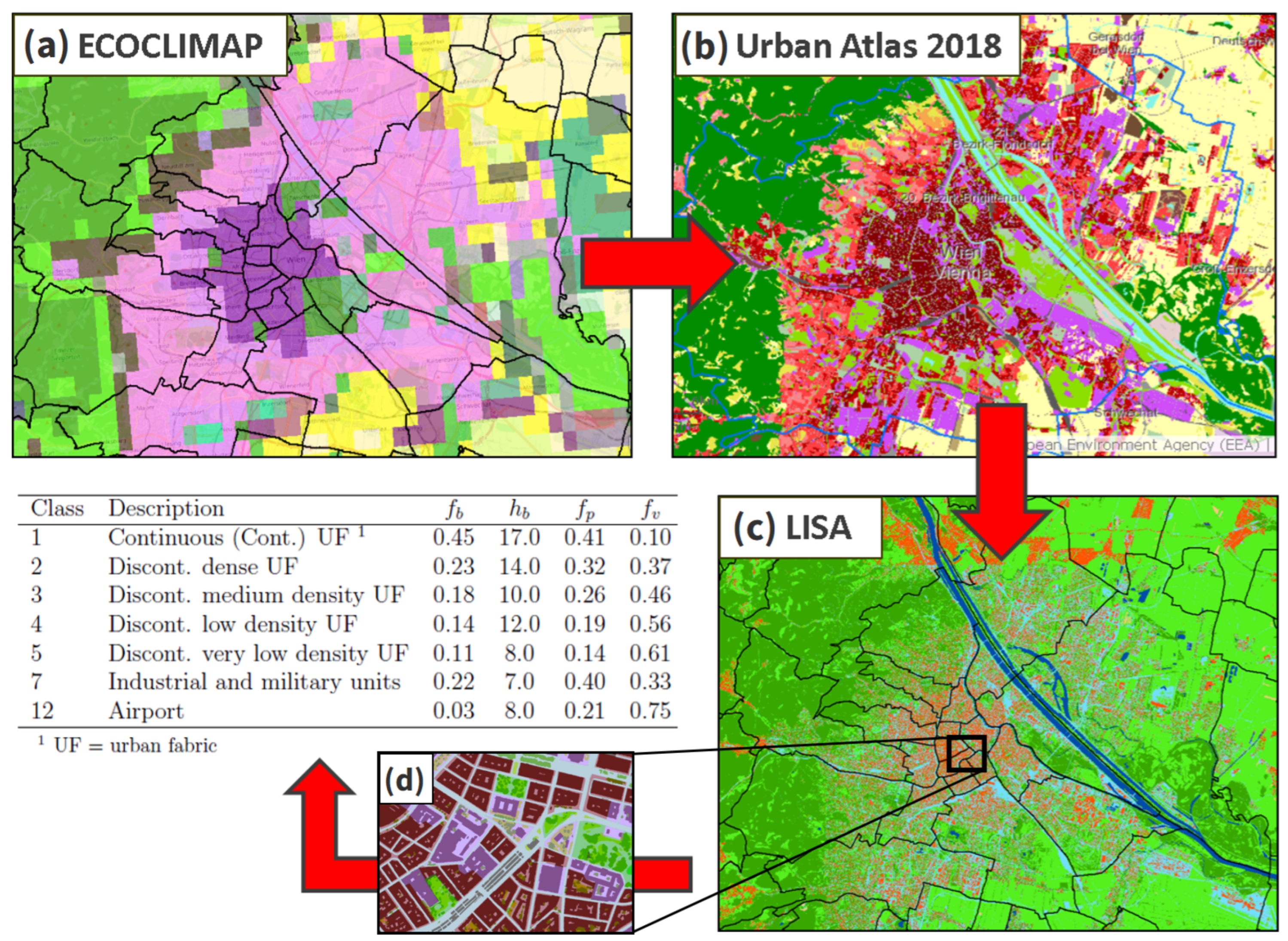
2.4. Land Use, Land Cover and Their Properties

For the surface model to accurately simulate temperature variations, it needs highly detailed land cover data. The Copernicus Land Monitoring Service portal, initiated by the European Environment Agency, provides more detailed land use information over major cities in the European Union in the form of UA. Each grid cell in SURFEX-SA was calculated with the percentage of each UA land cover class resulting in a possibility of 26 classes in one grid cell. The characterization of each UA class was hence made with LISA by a zonal statistics (ArcGIS) of the compromised 13 land cover classes (see Table S5 in the Supplementary Material). A schematic improvement of this process is given in Figure 2, where an exemplary table shows values from various fractions.

Table 2. Characteristic parameters for Urban Atlas land use classes in Vienna, Linz, Klagenfurt and Innsbruck where $f_b$ is the fraction of buildings and $f_v$ is the fraction of the vegetation cover. The table of all needed parameters (e.g., building height) for all cities are given in the Supplementary Material.

		Vienna		Linz		Klagenfurt		Innsbruck
Class	Description	${\mathit{f}}_{\mathit{b}}$	${\mathit{f}}_{\mathit{v}}$	${\mathit{f}}_{\mathit{b}}$	${\mathit{f}}_{\mathit{v}}$	${\mathit{f}}_{\mathit{b}}$	${\mathit{f}}_{\mathit{v}}$	${\mathit{f}}_{\mathit{b}}$	${\mathit{f}}_{\mathit{v}}$
11100	Continuous (Cont.) UF 1	$0.60$	$0.14$	$0.65$	$0.09$	$0.78$	$0.02$	$0.43$	$0.18$
11210	Discont. dense UF	$0.48$	$0.38$	$0.44$	$0.20$	$0.60$	$0.10$	$0.26$	$0.42$
11220	Discont. medium density UF	$0.36$	$0.54$	$0.34$	$0.28$	$0.40$	$0.22$	$0.21$	$0.49$
11230	Discont. low density UF	$0.26$	$0.69$	$0.14$	$0.52$	$0.13$	$0.46$	$0.10$	$0.68$
11240	Discont. very low density UF	$0.18$	$0.74$	$0.13$	$0.52$	$0.06$	$0.59$	$0.08$	$0.72$
12100	Industrial and military units	$0.38$	$0.30$	$0.38$	$0.19$	$0.25$	$0.24$	$0.22$	$0.38$
12210	Transit roads and AL 2	$0.07$	$0.22$	$0.11$	$0.26$	$0.09$	$0.30$	$0.03$	$0.54$
12220	Other roads and AL	$0.16$	$0.39$	$0.12$	$0.34$	$0.09$	$0.42$	$0.07$	$0.67$
12230	Railways and AL	$0.08$	$0.22$	$0.18$	$0.20$	$0.05$	$0.54$	$0.07$	$0.56$
12400	Airport	$0.06$	$0.63$	$0.07$	$0.51$	$0.02$	$0.01$	$0.04$	$0.72$
14100	Green urban areas	$0.04$	$0.84$	$0.12$	$0.66$	$0.10$	$0.56$	$0.12$	$0.60$
14200	Sports and leisure facilities	$0.11$	$0.75$	$0.10$	$0.65$	$0.04$	$0.69$	$0.05$	$0.76$
31000	Forest	$0.00$	$0.99$	$0.00$	$0.93$	$0.00$	$0.97$	$0.00$	$0.98$

¹ UF = urban fabric, ² AL = associated land.

provides the most important fractions of buildings and vegetation for each city. The Supplementary Material provides also a comparison between ECOCLIMAP-I and LISA considering the distribution of roads and railways in Vienna. Figure S1 shows how poorly ECOCLIMAP-I represents this type of LULC.

Implementing this huge amount of local information to create more realistic simulations in the urban canopy model requires also an update of other parameters such as the averaged building or tree height and the Leaf Area Index (LAI). This was achieved by utilizing several datasets:

(i) the building and tree height is based on data from the local governments using Digital Surface (DSM) subtracted from the Digital Elevation Models (DEM) along with masks from buildings and trees generated from LISA.

(ii) Vegetation parameters such as the LAI or the Normalized Difference Vegetation Index (NDVI) were obtained directly from Sentinel-2A reflectance bands 4 and 8 from 2022 (AMJJAS) pre-processed with Google Earth Engine to get a cloud-free image and updated in SURFEX-SA [57,58,59].

(iii) In a final step, we received information about the building age of each city to estimate the thermal properties of walls and roofs and averaged them per grid cell. To address the gap of missing building age information, we made assumptions based on available knowledge of the city administration.

The resulting data was then exported in the SURFEX-SA model, allowing it to incorporate the spatial distribution of various land cover types across the simulated urban area. This approach is supported by research from [60], which suggests that including sub-grid scale land use variability and initializing models with more precise land surface data leads to improved simulations of near-surface temperatures. Hence, we used a percentage distinction of UA classes per grid cell to account for the internal variability of land use. It means if a grid cell has 50% of class 11,100 in Vienna, the cell has only 30% of buildings for instance (see Table 2).

This combined approach facilitates the selection of the most effective model for future applications and offers several advantages over previous methods that relied solely on ECOCLIMAP and deterministic forecasts. The ability to quantify forecast uncertainty and incorporate more accurate land cover information is crucial for improving the overall performance of the coupled modeling system, especially at fine spatial scales.

2.5. Skill Scores

Various scoring rules have been proposed in the literature to evaluate the quality of forecasts. Governmental institutions and stakeholders, in their pursuit of informed decision-making, require accurate predictions of high-impact, unprecedented events [61]. The type of event determines the appropriate forecast format. For events with discrete outcomes, forecasts often take categorical or probabilistic forms. Categorical forecasts predict the most likely outcome, while probabilistic forecasts assign likelihoods to each potential outcome [62,63].

The Heidke Skill Score (HSS) is a popular metric for evaluating categorical forecasts. It assesses the accuracy of predictions based on the proportion of correct forecasts aligned with the highest probability assigned category. HSS ranges from $-0.5$ (worst) to 1 (perfect), indicating forecast discrimination, reliability, and resolution [64].

Another score, the Brier Score, a strictly proper scoring rule for probabilistic forecasts, calculates the squared difference between predicted $f_{br}$ and actual probabilities $y_{br}$ [65,66]. Its interpretability, simplicity, and bounded nature make it widely used. This metric assesses a forecast’s ability to discriminate between categories and avoid systematic biases in probability assignment. In essence, it evaluates how well forecasts distinguish the occurrence of an event and estimate its likelihood. If the expert’s Brier Score for an event is denoted as $BrS$, the corresponding fair Brier Score $fBrS$ can be calculated as

$$fBrS=BrS\ast (B-1)/B=\sum _{br=1}^B{(f_{br}-y_{br})}^2\ast (B-1)/B.$$

(1)

The adjustment term $(B-1)/B$ represents the expected score of a forecaster who makes predictions based on the principle of insufficient reason, also known as the ‘principle of indifference’ [67]. This forecaster assumes all possible outcomes are equally likely and assigns a probability of $1/B$ to each outcome. The fair Brier score, therefore, quantifies the added accuracy of a given forecast compared to this baseline of an unskilled forecaster [68].

The Faction Skill Score (FSS) is a popular metric for evaluating the accuracy of spatial forecasts. Based on the huge amount of NETATMO data, we generated 2D air temperature fields and thus were able to apply the FSS here as well. It compares the fraction of grid points exceeding a specified threshold in a forecast and an observed field. A perfect forecast achieves an FSS of 1, while a ‘no skill’ forecast scores 0. The denominator in the FSS calculation significantly influences its characteristics. For instance, the FSS is undefined when neither the forecast nor the observed field exceeds the threshold. An important limitation of the FSS is its symmetry. It cannot distinguish between false alarms (incorrectly predicting an event) and misses (failing to predict an event). This is due to the fact that the FSS is 0 if either the forecast or the observed field does not exceed the threshold [69].

2.6. Verification Methods

As described before, the 00 UTC forecast of SURFEX-SA is finished every day at around 05 UTC. Hence, the operational weather service can only use lead time from $+6$ till $+30$ h to estimate potential temperature warnings on that or the following day.

In this manner, we analyzed the leading 25 h after 05 UTC using the mean bias (model minus observation), the root mean squared error (RMSE), the mean absolute error (MAE) and the before described skill scores.

To account for potential biases in air temperature measurements due to local environmental factors (e.g., parked cars, roadwork) that may affect TAWES or NETATMO observations, we used the weighted average of the temperature calculated by the TEB and ISBA models.

We used R and the R tool ‘harp’ for the point and spatial verification. The ‘harp’ framework is used for NWP analysis, verification and visualization has been developed by the ACCORD consortium [70]. The advantage of harp is the universal reading function for file types such as .nc, .fa or .grb and it requires as input only the coordinates of the weather stations (in our case TAWES and NETATMO) and the respective measurements.

However, when interpreting the biases and various scores, two aspects must be considered in our case:

(i) The atmospheric forcing is the same for both the $2.5$km and $100$m model grids, even though mathematical interpolation is used to get the $100$m grid values. This means that the variability in temperature between the canopy vegetation temperature T2M_ISBA ($0.76$ K) (see Figure 3a) and T2M_TEB ($0.59$ K) (see Figure 3b) for the $100$m grid in SURFEX-SA within this specific area is relatively small. Only through the weighted averaging of T2M_ISBA and T2M_TEB more realistic patterns (e.g., parks within the city are significantly cooler) appear in the temperature field (Figure 3e) compared to the homogeneous $2.5$km grid cell in AROME (Figure 3d). However, this effect cannot be detected with a point validation, since the point measurement is also compared with a grid cell value that does not capture the whole microclimate within a grid cell. To validate the modelled temperature field, one needs a denser monitoring network of stations representative for urban conditions like NETATMO (see Section 2.7). Hence, we have adopted a strategy of resampling the CWS measurements onto a uniform grid to ensure a fair, spatial comparison between the model output and the huge amount of local observations. This resampling output can be used for the FSS. Detailed information about this interpolation is given in the Supplementary Materials.

(ii) It is questionable, which modeled air temperature should be compared with the station measurement. Stations located according to World Meteorological Organization criteria are more likely to comply with T2M_ISBA, as they measure over grass and not over sealed ground.

The value that is interesting when modelling urban heat islands, on the other hand, is actually T2M_TEB, for which there is usually no corresponding station measurement. Figure 4 shows the measurement for a TAWES station in Vienna as well as the SURFEX-SA forecast for 16 August 2022 of T2M_ISBA, T2M_TEB and T2M. The stronger diurnal cycle of T2M_TEB is clearly visible, which leads to a difference between T2M_TEB and T2M_ISBA of up to $3$K being modeled for the same grid cell.

2.7. Quality Control of Citizen Weather Stations

To enlarge the number of measurements against which the model results can be compared, we also incorporated citizen weather stations in our analysis.

For that purpose, we used temperature measurements from the NETATMO network, since they were successfully applied and analyzed by several studies previously [45,72,73,74,75,76,77,78]. NETATMO weather stations consist of an indoor and outdoor module, with the air temperature sensors being inside an aluminum case. Data can be retrieved from the website using an API, as described e.g., in [73]. The data used here, however, was acquired directly from the company NETATMO.

While citizen weather stations have the huge advantage to provide a dense monitoring network, they cannot be used without a thorough quality control (QC) [44,46,73,79,80]. The work of [46] combined the approach from [44,73] to perform a QC of NETATMO air temperature data for the city of Vienna. Given those promising results, we adopted the same approach, but incorporated an additional QC step and applied the further developed R package CrowdQC+ [47] instead of CrowdQC [81] to perform the first six QC steps, which do not require reference data. The last two QC steps were included to reduce remaining radiative errors and are based on [73]. The reference data needed for the last two QC steps comprise global radiation and 2 m temperature measurements from TAWES weather stations. The QC was carried out on a monthly basis and the initial QC steps are described in [46].

The additional QC step, which is carried out after L4 and before L5 in [46], is the spatial buddy check. It was incorporated into the CrowdQC+ package to reduce remaining erroneous data, mainly radiative errors, and performs a statistical outlier detection among neighboring stations [47]. Isolated stations (less than five neighboring stations within a $3$km radius) were flagged as isolated but passed the QC step to ensure that enough stations for the verification remain, especially in data sparse regions.

In our study, most NETATMO stations are available for Vienna, with 1291 stations passing the QC in June/July 2019 followed by Linz (424), Innsbruck (214) and Klagenfurt (112). It should be noted that the availability of NETATMO data varies with time, due to e.g., interrupted Wi-Fi connections [45] and the QC procedure, which filters out single values as well as entire stations.

3. Results

This Section presents (Section 3.1) a seasonal perspective of SURFEX-SA compared to AROME for low (December and January) and high (July and August) air temperatures in 2023/2024 with TAWES measurements (in sum 44 stations) to evaluate the model performance and improvement using detailed LULC input data, (Section 3.2.1) a heat wave in 2019 using TAWES and NETATMO observations to demonstrate how well SURFEX-SA represent the extreme temperatures in urban environments and finally (Section 3.2.2) a use case of 2023 with an intense tropical night using C-LAEF and TAWES measurements estimating of uncertainties in model predictions.

3.1. Seasonal Evaluation

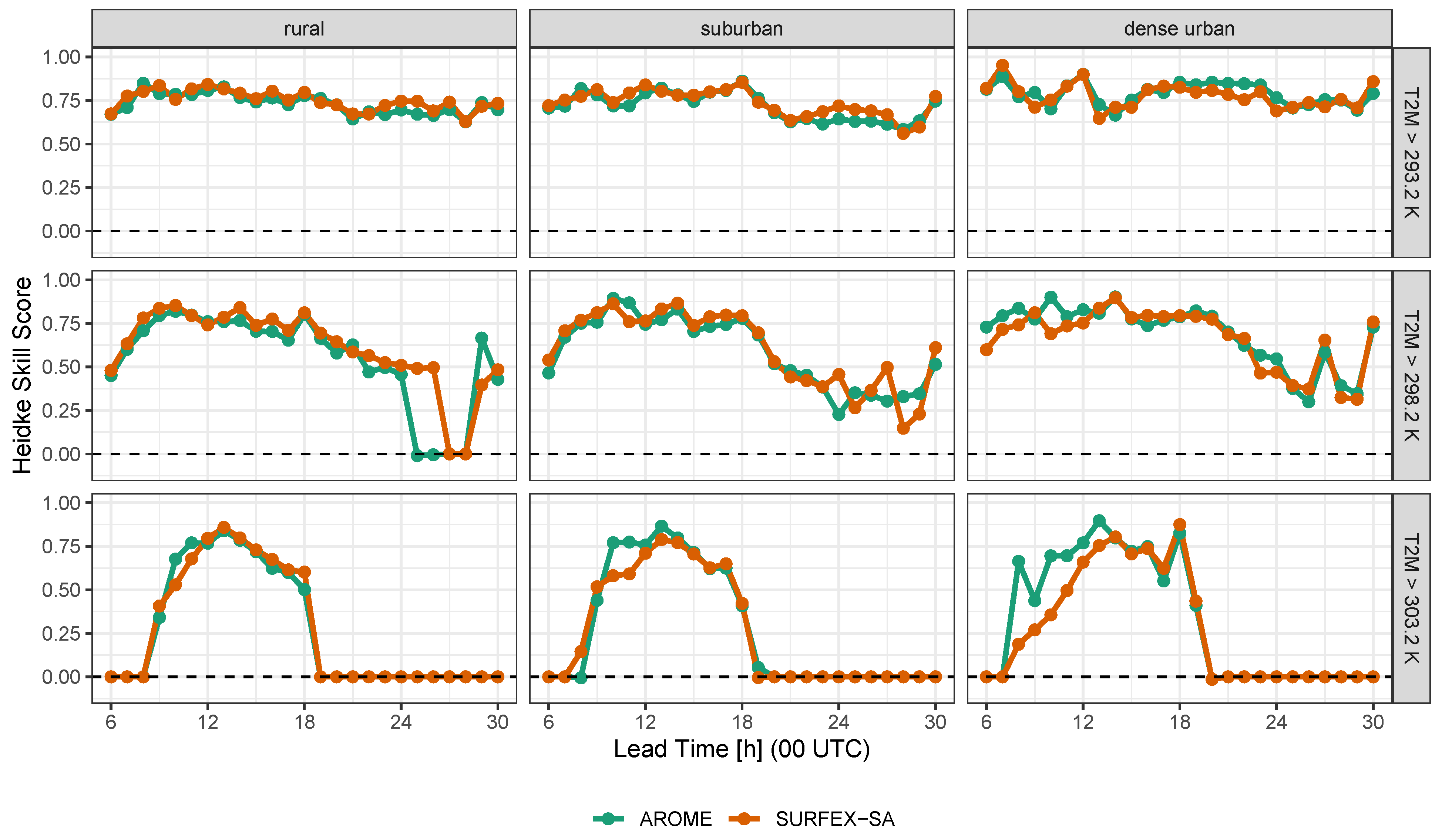
3.1.1. Summer Season

In a first step, we looked into the summer of 2023 with 5 to 7 heat waves (depending on the city) between July and August. Due to the large model-domains, covering the city as well as its surroundings, we split up the statistical values in three categories of urban environments in direct vicinity of TAWES stations (depending on vegetation fractions within the specific grid cell that comprises the TAWES station) with rural (>70%), suburban (between $30\%$ and $70\%$) and dense urban (<30%). This distinction results in at least 2 stations per category and city, and allows to investigate how well the SURFEX-SA/AROME forecasts are regarding the maximum (usually in city centers) or minimum (usually in rural areas) of T2M.

Figure 5 shows the result of the here proposed statistical parameters and reveals one uniform picture considering the daily maximum. In each city the RMSE and MAE are highest between 12 and 17 UTC. This shows a clear under or overestimation of T2M (depending on the model domain) already in AROME, which affects SURFEX-SA predictions, as they depend on the forecast quality of AROME. Regarding the different urban environments, the verification yields sometimes a complete different picture. Figure 5a shows Vienna with a pronounced overestimation of T2M in dense urban areas during daytime and an overestimation in rural areas, whereas in Linz (Figure 5b) SURFEX-SA underestimated the air temperature in rural areas during the whole forecast. In Klagenfurt and Innsbruck, the bias shows a different impression of SURFEX-SA where it has lower values for sub- or dense urban areas during nighttime (Figure 5c,d).

However, the first seasonal comparison between AROME and SURFEX-SA does not show a need for high-resolution T2M forecasts in the summer season. AROME is for the most part close to zero or better than SURFEX-SA except for suburban areas around Innsbruck during nighttime.

A more clear (dis)advantage of SURFEX-SA compared to AROME shows the Heidke Skill Score (HSS). Figure 6 provides the HSS for AROME and SURFEX-SA in Vienna and surroundings with the three urban environments in the columns and three important air temperature thresholds as $293.2$K (tropical night), $298.2$K (summer day) and $303.2$K (hot day) chosen based on the recommendations of the Expert Team on Climate Change Detection and Indices (ETCCDI) [82] and the potential of triggering human thermal stress [83,84].

Considering the heat burden during daytime, the HSS shows a slightly better performance of AROME compared to SURFEX-SA due to the slower heating up of the latter before noon. In the rest of the day, both yield almost the same range between $0.5$ and $0.88$ for lead times $+6$ till $+18$. The threshold of summer days shows a similar picture with HSS values up to $0.9$. However, the HSS of the tropical night threshold represents a contrary output where SURFEX-SA has a slightly better performance between 21 and 04 UTC, especially in rural and suburban areas. This moderate advantage of SURFEX-SA can also be seen in Figure 5a with the lowest MAE during nighttime.

In Figure 7a, a similar result of HSS is revealed for the city of Linz and the surrounding area. AROME is most of the time slightly better, even in suburban areas above $293.2$K during nighttime. The perfect score of $\mathrm{HSS}\ge 0.65$ in rural areas between 20 and 23 UTC is the only time period when SURFEX-SA outperforms AROME.

Looking to the southern part of Austria, Klagenfurt (Figure 7b) shows a decrease in number of situations where T2M $>303.2$K and AROME is in most cases slightly better than SURFEX-SA again. Whereas the bias and RMSE/MAE in Figure 5c shows that SURFEX-SA has a better output for sub- and dense urban areas, the HSS of SURFEX-SA in Figure 7b has lower values regarding the capture of tropical nights. Those skill scores can be used to evaluate the performance of the forecasts, however, only at the TAWES stations. Regarding the given results, SURFEX-SA does not seem to perform better than AROME at those points.

Figure 7c presents the lowest values of HSS for the city of Innsbruck and surroundings. Similar to greater bias and high errors in Figure 5, AROME as well as SURFEX-SA show limitations to predict T2M properly above $303.2$K. The values of HSS for SURFEX-SA during summer days and tropical nights show the lowest of all cities and demonstrate the need of AROME model improvements in areas with mountains.

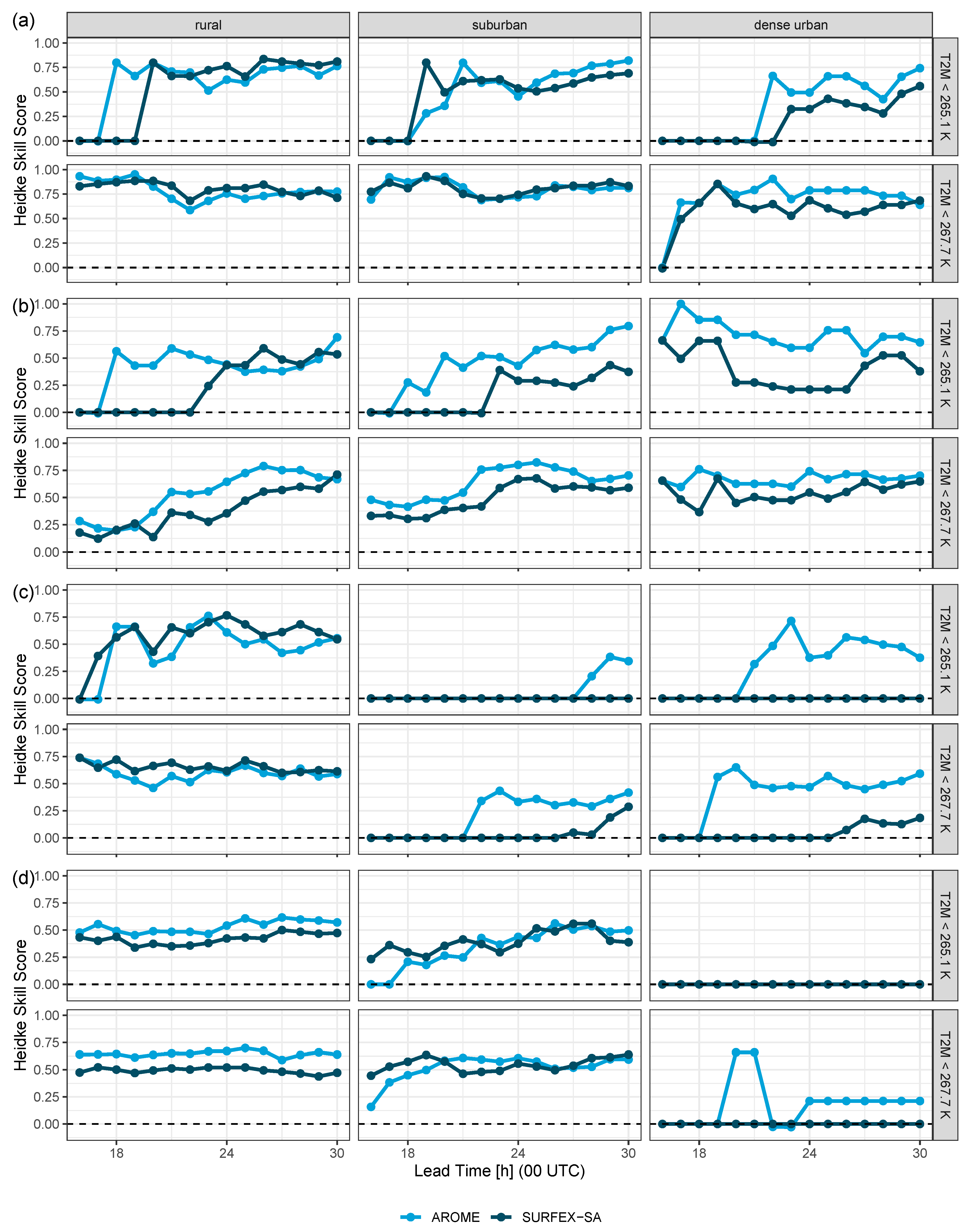
3.1.2. Winter Season

In the case of extreme low temperatures, we analyze the winter season 2023/2024 for the months December and January. As February 2024 was one of the warmest Februaries in Austrian history, we excluded this month in the analysis. During this period, some extreme cold waves appeared in December and January, with the lowest T2M in the forecast domain being $258.1$K (measured in Hoersching near Linz, at height above sea level of $298$m).

Figure 8 shows again the hourly mean bias, the RMSE and the MAE of AROME and SURFEX-SA but only for lead time $+16$ till $+30$ (i.e., 16 UTC till 06 UTC on the following day) due to the consideration of very low temperatures. As the UHI effect is more pronounced in the winter season than during summer season, it might be interesting to see the distinction between the three urban environments. However, Figure 8 represents a similar picture as in the summer season. SURFEX-SA has its benefits only in the suburban areas of Innsbruck with a bias of approx. $0.25$K and the lowest RMSE/MAE (see Figure 8d). All other panels show the almost identical values of RMSE and MAE (Figure 8a–c), except for the city of Vienna where T2M in dense urban areas is crucially underestimated by SURFEX-SA. A reason for this could be wrong initial model settings or specific wind conditions at the TAWES stations, but will not be discussed in this manuscript.

The HSS was analyzed again for all pilot cities but, of course, with different thresholds. Due to the higher temperatures in urban environments, we chose the thresholds of $265.1$ and $267.7$K based on the measured monthly minimum T2M averaged over all four city centers for December and January, respectively.

Figure 9 shows the HSS for all cities. Figure 9a presents Vienna with a nearly equal performance between AROME and SURFEX-SA for both thresholds within rural and suburban areas, whereas dense urban areas are better predicted by AROME for the whole nighttime.

Although SURFEX-SA has a bias of ≃0 K within dense urban areas in Linz, the HSS in Figure 9b shows a complete different picture. Threshold $265.1$ as well as $267.7$K are represented poorly by SURFEX-SA compared to AROME ($\Delta \mathrm{HSS}$ up to $0.5$ between them). A similar picture is also given in rural and suburban environments. Hence, the proportion of T2M forecasts by SURFEX-SA correct by chance is 20 to $50\%$ lower than by AROME. Such results demonstrate the need of skill scores and deeper validation than simple statistical values.

SURFEX-SA performed in Figure 9c for Klagenfurt and surroundings also with low values of HSS and is most of the time below (or even zero) the skill score of AROME. Only in rural areas, SURFEX-SA shows a better performance compared to AROME (see also the bias in Figure 8c).

Last but not least, both numerical models have a weak performance in Innsbruck and rarely capture air temperatures below $265.1$K (although such temperatures were measured in the city center during both months).

These results clearly show the need to improve extreme low temperature forecasts (focused on dense urban areas) during the winter season for AROME and SURFEX-SA as extreme temperatures occur in both seasons.

3.2. Case Studies of Extreme Temperatures During Summer Season

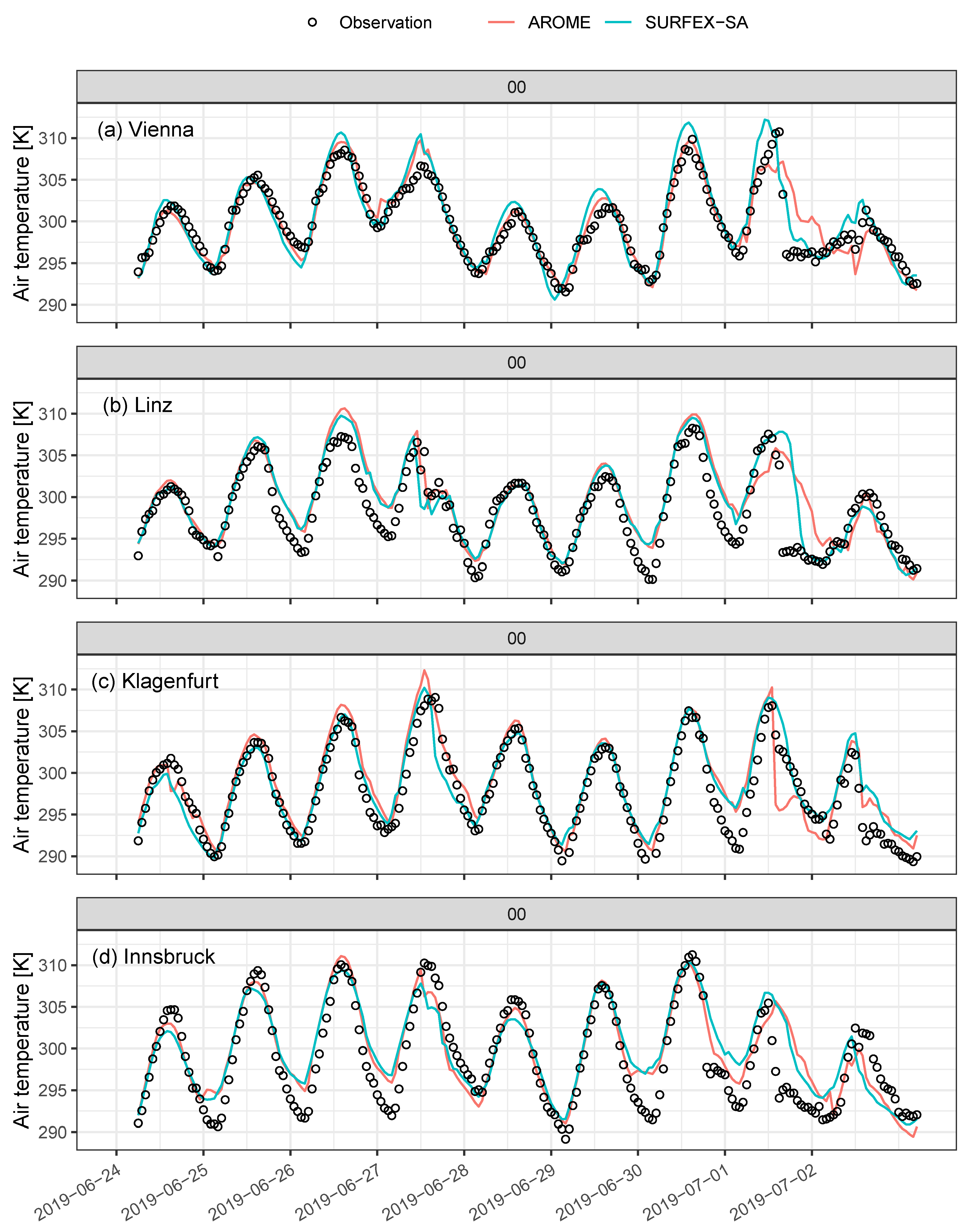
An additional approach to analyze the added value of SURFEX-SA to AROME, we chose specific heat waves in 2019 and 2023. In this manner, we want to characterize the model performance for each city and its surroundings as much as possible using TAWES stations as well as the dense station network from NETATMO.

3.2.1. Year 2019

To investigate one of the strongest heat waves in the last decade, we recalculated AROME for June and July of 2019. In this period, T2M reached >310.2 K in Vienna on two consecutive days and on one of these days in Innsbruck (measured by TAWES stations, respectively). Figure 10 shows the extreme heat wave between 24 June and 3 July for the city center of all four cities. Notably, Linz (panel b) and Klagenfurt (panel c) reached more than $308.2$K on 30 June and 27 June, respectively. At a first glance, AROME and SURFEX-SA capture the measurements quite well most of the time. However, minima and maxima are under- or overestimated in some cases and will be analyzed in the following section.

As in Section 3.1, the HSS was calculated of AROME and SURFEX-SA compared to all available TAWES stations again, but only for lead time $+13$ till $+15$ h (usually maximum T2M) and $+26$ till $+28$ h (usually minimum T2M). To evaluate the performance of SURFEX-SA compared to AROME in various heights above sea level (as the spatial resolution of SURFEX-SA is much higher), we distinguish between two height thresholds depending on the height above sea level of each city. Figure 11 shows the HSS for both models. SURFEX-SA performs better in Vienna and Innsbruck for desert days (T2M $>308.2$K). In Linz and Klagenfurt, AROME has the same or even a better score for both temperature thresholds.

Figure 12 presents the performance of both models considering the high number of tropical nights during this period. At the lower threshold of $291.2$K (average value where tropical nights did not occur), we see that SURFEX-SA outperforms AROME only in Linz (both heights) and Innsbruck (≥500 m). However, the more important threshold of $293.2$K was captured much better by SURFEX-SA in Linz, Klagenfurt (≥500 m) and Innsbruck (<700 m).

In order to evaluate spatial variations and model performance in various urban environments, QC NETATMO data are used for the statistical verification. Figure 13 provides the averaged T2M difference between SURFEX-SA and NETATMO observations at lead time $+13$ for each pilot city as SURFEX-SA predicts the daily minima quite well (see Figure 14 after lead time $+24$). Similar to the previous results, we summarize the following:

(i) SURFEX-SA overestimates the T2M between $+2$ and $+4$K in Vienna and surrounding areas in approx. $32\%$ of the measurement points, whereby few of them reach differences of ≥±6 K (see Figure 13a). However, the relatively high number of differences <±2 K allows the interpretation of a smaller bias similar given in Figure 5a compared with TAWES measurements. The statistics with NETATMO data in Figure 14a confirms this output where the RMSE and MAE vary around $+2$K.

(ii) The city of Linz and surrounding areas yield a result in which the majority of the NETATMO measurements are higher than the modeled output from SURFEX-SA. Figure 13b shows the underestimated T2M, especially in rural areas with a maximum difference of $+6.9$K. These results are consistent with the analysis with the TAWES measurements of July–August 2023 (see Figure 5b), where rural areas are clearly underestimated by SURFEX-SA during the afternoon. However, sub- or dense urban areas within Linz (districts in black polygons) do not show the slight overestimation of SURFEX-SA (≃1 K) at 13 UTC as in Figure 5b and provide more points with a negative difference (see Figure 14 with a bias of $-1$K).

(iii) Figure 13c shows a good agreement of SURFEX-SA compared to the NETATMO measurements at 13 UTC, where there is only one point with a bias of ≥−6.2 K (southernmost point in the domain). Hence, Figure 14c shows a bias of $-0.5$K and a RMSE of ≃2 K. However, the bias and RMSE / MAE increase to $-2.5$ K or $3$ K until 18 UTC. This kind of variation can also be seen in Figure 5c, where both (AROME and SURFEX-SA) decrease in bias from lead time 13 until 18 h. This is a perfect example for the fact that SURFEX-SA intensified the signal of AROME, and hence, SURFEX-SA can not compensate for the wrong forecasts of AROME.

(iv) Model results for the city of Innsbruck presents the highest values of maximum difference, RMSE and MAE with $9.8$K, $4.4$K and $4.1$K (see Figure 14d). The strong underestimation of T2M from SURFEX-SA is well presented in Figure 13d. Dense urban (city districts inside the southern polygons) as well as rural areas show a negative averaged bias of $-1.3$K at 13 UTC. As described before, AROME already underestimates the T2M (see Figure 5d) and this can not be compensated by high-resolution land cover data or adapted model configuration.

An overall statistical comparison between SURFEX-SA and NETATMO observations for all pilot cities and the study period 24 June till 3 July 2019 is given in

Table 3. Statistical verification of modelled air temperature with quality-controlled data from NETATMO citizen weather stations in the study area, respectively. Average difference (bias), standard deviation (${\sigma }_{\mathrm{mod}-\mathrm{obs}}$), maximum difference ($|{\Delta }_{max}|$), root mean square error (RMSE) and mean absolute error (MAE) for the study period 24 June till 3 July 2019 06 UTC.

	Vienna	Linz	Klagenfurt	Innsbruck
Nr. of data	209,512	67,879	19,462	36,414
Bias	$0.9$	$0.5$	$-0.7$	$0.0$
${\sigma }_{\mathrm{mod}-\mathrm{obs}}$	$1.5$	$1.6$	$1.7$	$1.7$
$|{\Delta }_{max}|$	$11.3$	$14.9$	$15.2$	$11.4$
RMSE	$2.1$	$2.4$	$2.6$	$2.8$
MAE	$1.7$	$2.1$	$2.2$	$2.4$

. It shows in sum similar results as in Section 3.1, where SURFEX-SA overestimated Vienna and Linz, and underestimated Klagenfurt (bias) in extreme high air temperature events. Maximum differences of up to $15.2$K are not interpreted here as they need more investigation considering model or measurement problems. The RMSE/MAE values in this table show the accordance to the seasonal evaluation in 2023 again (see Figure 5). The presence of complex mountainous terrain deteriorates the accuracy of the simulated air temperature in both models.

In the last step of the comparison with NETATMO data, we calculated the FSS to see how well SURFEX-SA represents the air temperature spatially. Figure 15 and Figure 16 represent the FSS as a maximum value for each day in the regarding heat wave of 2019. The maximum FSS is chosen to see highest possible score of SURFEX-SA within the whole modeling domain and hence, the maximum added value of high-resolution forecasts.

Figure 15a,b presents the FSS of Vienna and Linz between 13 and 15 UTC for each day during this heat wave, respectively. In Vienna (Figure 15a), SURFEX-SA performs quite well with a FSS of ≥0.87 at the air temperature threshold of >303.2 K, where it occurs on several days. However, at the next threshold (>308.2 K) SURFEX-SA yields values between $0.41$ and $0.95$. As described in the work of [85], FSS values above $0.5$ indicate a useful skill and hence, SURFEX-SA has only one case where it is below this reference value. As expected, we see the lowest values of FSS at highest threshold with >310.2 K. Such rare measured air temperatures were only captured by SURFEX-SA in the case of 1 July, where all neighborhood radius have values of ≥0.51. Other days as 26 June and 30 June represent values below $0.5$, however, increase it with higher radius.

Although SURFEX-SA underestimates T2M at several NETATMO stations at 13 UTC in Linz and surroundings (see Figure 13b), it reaches values between $0.62$ and $1.00$ at all grid box radius and thresholds on 25, 26, 30 June and 1 July (see Figure 15b). The other days during this heat wave were captured poorly by SURFEX-SA, but these result shows that a simple averaged bias between model outputs and observations does not reveal the added value of high-resolution forecasts in extreme temperature cases.

Figure 16 presents the same schematic results of FSS but for the cities of Klagenfurt and Innsbruck and their surroundings. In the most cases of Klagenfurt, SURFEX-SA yields a moderate FSS of ≥0.5 (see Figure 16a). However, the highest threshold of $309.2$K were obtained with only values below $0.21$ by SURFEX-SA.

The model domain of Innsbruck and surroundings has the overall lowest FSS of all pilot cities with values varying between $0.23$ and $0.65$ in Figure 16b. The highest temperature threshold of $310.2$K were captured only once by SURFEX-SA (26 June 2019), although it were measured in the city center on three days in the considered time period (see Figure 10d). Furthermore, SURFEX-SA reaches moderate or useful skill scores at the lowest threshold ($303.2$K) leading to a practical forecast system on at least hot days in complex areas.

Such values do not represent a weak model performance but have to be handled carefully due to neighbourhood radius and its smoothing with more than one NETATMO station (increasing FSS with increasing grid boxes), which can be set up completely different regarding urban environments.

3.2.2. Using C-LAEF in 2023

In this example, we want to analyze the added value of the ensemble prediction system C-LAEF ($+60$h) as described in Section 2.1. Therefore, we chose 23 June 2023 where one of the warmest tropical night happened with a minimum measured air temperature of $297.7$K in the city center of Vienna.

Figure 17 shows the forecast of SURFEX-SA for two different time stamps (lead time $+30$ and $+36$ starting from 22 June 2023, 00 UTC) as ensemble average (left) and their standard deviation (right). The average T2M of 06 UTC depicts the tropical night over the whole city, which was captured by the ensemble members quite well although we recognize an overestimation of the daily maxima in the model (see time series at the bottom in Figure 17). The second time stamp below was captured by only 3 members, which shows, however, the possibility to predict the air temperature in a right way with C-LAEF. The standard deviation on the two right panels provides also the possibility to see variation of ensemble members over the whole domain. Whereas the northern part shows a standard deviation of <2 K, the southern part reflects a greater spread, including urban and rural areas.

In a final step, we apply a score analysis on both models again but with the Fair Brier Score $fBrS$ due to the ensemble forecast. Unlike the Heidke Skill Score, which focuses on categorical accuracy, the $fBrS$ measures the squared error between forecast probabilities and observed outcomes (see Section 2.5).

Figure 18 shows the $fBrS$ for, again, three different urban environments and now, for four different air temperature thresholds as we analyze the forecast quality on an enhanced time period of 54 h. Both models (C-LAEF and SURFEX-SA) seem to be quite near at the scores range above the thresholds of $293.2$ and $298.2$K. The only exception is the rural and suburban environment, where SURFEX-SA yields a double high value at the lead time $+7$h and at $+31$h in only rural areas.

However, if we behold the higher values of T2M with $300.2$ and $305.2$K, the $fBrS$ reveals a much better performance of SURFEX-SA compared to C-LAEF. Lead times $+12$ till $+17$ and $+33$ till $+39$ (afternoon of the first 2 days) show higher values of $fBrS$ for all urban environments and yield the real added value of SURFEX-SA. We see that SURFEX-SA used in an ensemble system predicts higher air temperatures much better than C-LAEF itself.

4. Discussion

While the results of this study demonstrate the potential of high-resolution forecasts for urban hot and cool spots, several aspects require further investigation.

Firstly, the availability of accurate and up-to-date LULC data is crucial for the effectiveness of these models. Datasets like LISA and UA, while valuable, may not always reflect the most recent changes in urban land use due to, e.g., a grow of sealed areas of $41{\mathrm{km}}^2$ in entire Austria every year [86]. More recent land cover maps such as the CORINE land cover (CLC+ Backbone) [87] or the European Space Agency World Cover [88] in $10$m spatial resolution from 2021 or the GlobeLand30 [89] in $30$m spatial resolution from 2020 could have been used but do not provide a distinction between buildings and streets or are too coarse. Future studies should explore the use of more recent and detailed LULC data, including incorporating satellite imagery and laser scan measurements. A promising algorithm is provided in the recent work of [90] with a Cross-Resolution Land-Cover Mapping framework leveraging noisy label learning to utilize existing low-resolution, potentially inaccurate land-cover data to generate new, higher-resolution land-cover maps.

In addition, SURFEX-SA is limited by the design of an urban canyon. Microclimatic effects can not be captured as the horizontal advection is not simulated in SURFEX-SA and each grid box represents only a schematic urban canyon with the percentage of buildings, streets, vegetation and/or water. This urban canyon is also averaged in terms of short- and longwave radiation as the road direction in TEB is not given and hence, it rotates the street through $360°$ with a $5°$ step.

Secondly, the comparison between model-predicted and station-measured temperatures may be influenced by the specific characteristics of the measurement locations. Station measurements over vegetated areas such as always given by TAWES and sometimes also by NETATMO may align more closely with model outputs over large homogeneous vegetated areas, due to the absence of microclimate effects. For urban heat island studies, a combined temperature over both sealed and vegetated areas is more relevant. However, the lack of corresponding station measurements in these areas poses a challenge. Future studies could address this by establishing a network of stations specifically designed for urban heat island research or use new Machine Learning methods as described in [91].

In addition, the choice of spatial resolution may be more significant than anticipated. The study of [92] showed a similar coupled NWP system with AROME and SURFEX at $1$km resolution. It found an average RMSE of $1.49$K within 5 years of observations during JJA at 5 weather stations in the city of Stockholm. This value is moderate lower than any RMSE found in the present work. Hence, such differences in the spatial resolution can affect the models output through the encompass of diverse microclimatic effects and should be evaluated in future (sensitivity) studies.

Finally, future improvements to SURFEX-SA including further development of TEB could enhance its representation of urban complexities. The integration of Building Energy Models (BEMs) would allow simulating the effects of building design and energy efficiency strategies on urban temperatures. In addition, advancements in SURFEX-TEB v9.0 include improved representation of trees within urban canyons and multi-layer coupling between high-rise buildings and the surrounding atmosphere as used in [40]. In this way, SURFEX-SA has the potential to outperform AROME if the model settings and the LULC information are accurate enough.

5. Conclusions

This study investigates the effectiveness of a coupled modeling system, AROME and the stand alone SURFEX-SA, in predicting air temperatures at high resolutions ($2.5$km to $100$m) in four Austrian cities. The system was computing forecasts on a daily base for approximately two years leading to evaluate the added value of incorporating detailed urban environmental representations. The analysis focused on the years 2019, 2023, and 2024, examining both summer and winter seasons.

Accurate LULC information, essential for SURFEX-SA, was initially derived from the Urban Atlas dataset. However, a more detailed LULC map was created using LISA data, building/tree height information, and vegetation indices. The evaluation of SURFEX-SA involved comparing its predictions to measurements from Austria’s weather monitoring network (in sum 44 stations) and quality-controlled data from the NETATMO CWS network. SURFEX-SA demonstrated improved performance in specific situations, particularly during nighttime in rural and suburban areas during the warmer season. Furthermore, we saw a better Heidke Skill Score from SURFEX-SA during the heat wave of 2019. The verification with NETATMO citizen weather station measurements considering averaged statistical values reveal a similar performance of SURFEX-SA compared to summer season evaluation with TAWES observations. Hence, SURFEX-SA allows a promising high-resolution air temperature forecast in extreme situations, where dense urban environments exist and AROME can not capture those structures. In conclusion, we outline as follows:

• The physical downscaling of Vienna’s urban climate using the AROME/SURFEX-SA system, exhibiting an average MAE of $1.4$ and $1.7$K (summer and winter) against 4 months of hourly observations at 14 operational weather stations, has demonstrated the necessary performance for this study’s objectives. The work of [40] showed similar results in terms of biases and RMSE during a heat wave in Hong Kong, China.
• Due to the better forecast quality of SURFEX-SA in combination with the ensemble forecasting system C-LAEF presented in this study, it is obvious that such prediction of air temperature lead to a kind of monitoring system for city planners and stakeholders. Past extreme heat waves can be evaluated by those identifying city areas with enhanced occurring heat loads.
• While SURFEX-SA shows better forecast skills in summer compared to AROME, AROME provided comparable or superior predictions during the cold season as analyzed in December–January 2023/2024. Such discrepancies in forecasts yield to further sensitivity analysis regarding physical processes within the models and various spatial resolutions. However, integrating this aspect here extends beyond the scope of this study due to the comprehensive modules and model configurations in both models.
• A further aspect is the dissemination of high-resolution forecasts to vulnerable citizens and city governments, which is essential for their practical application. Developing user-friendly apps and integrating these forecasts into national weather services and warning systems would improve accessibility. However, it is important to note that the need for high-resolution forecasts may be limited to extreme temperature situations.
• Nevertheless, it is worth noting that the establishment of a physical downscaling system utilizing SURFEX-SA forecasts, leveraging the LULC knowledge acquired in this study, is a feasible endeavor. The advantages of this system compared to the basic AROME forecasts were just visible in spatial details and extreme heat situations. We assume the potential to add additional skill to the SURFEX-SA forecasts with recent developments in SURFEX-TEB v9.0, that is available just after this study was finished.

References

1. IPCC, Intergovernmental Panel on Climate Change. Climate Change 2022—Impacts, Adaptation and Vulnerability: Working Group II Contribution to the Sixth Assessment Report of the Intergovernmental Panel on Climate Change; Cambridge University Press: Cambridge, UK, 2022. [Google Scholar] [CrossRef]
2. Fischer, E.M.; Schär, C. Consistent geographical patterns of changes in high-impact European heatwaves. Nat. Geosci. 2010, 3, 398–403. [Google Scholar] [CrossRef]
3. Molina, M.O.; Sánchez, E.; Gutiérrez, C. Future heat waves over the Mediterranean from an Euro-CORDEX regional climate model ensemble. Sci. Rep. 2020, 10, 8801. [Google Scholar] [CrossRef] [PubMed]
4. Landsberg, H.E. The Urban Climate; Elsevier Science: Stanford, CA, USA, 1981. [Google Scholar]
5. Oke, T.R. The energetic basis of the urban heat island. Q. J. R. Meteorol. Soc. 1982, 108, 1–24. [Google Scholar] [CrossRef]
6. Zhou, B.; Rybski, D.; Kropp, J.P. The role of city size and urban form in the surface urban heat island. Sci. Rep. 2017, 7, 4791. [Google Scholar] [CrossRef]
7. Macintyre, H.L.; Heaviside, C.; Cai, X.; Phalkey, R. The winter urban heat island: Impacts on cold-related mortality in a highly urbanized European region for present and future climate. Environ. Int. 2021, 154, 106530. [Google Scholar] [CrossRef] [PubMed]
8. Lauwaet, D.; Berckmans, J.; Hooyberghs, H.; Wouters, H.; Driesen, G.; Lefebre, F.; De Ridder, K. High resolution modelling of the urban heat island of 100 European cities. Urban Clim. 2024, 54, 101850. [Google Scholar] [CrossRef]
9. APCC14. Austrian Assessment Report Climate Change 2014 (AAR14); Austrian Panel on Climate Change (APCC): Vienna, Austria, 2014. [Google Scholar]
10. Oswald, S.M.; Hollosi, B.; Žuvela Aloise, M.; See, L.; Guggenberger, S.; Hafner, W.; Prokop, G.; Storch, A.; Schieder, W. Using urban climate modelling and improved land use classifications to support climate change adaptation in urban environments: A case study for the city of Klagenfurt, Austria. Urban Clim. 2020, 31, 100582. [Google Scholar] [CrossRef]
11. Žuvela-Aloise, M.; Andre, K.; Schwaiger, H.; Bird, D.N.; Gallaun, H. Modelling reduction of urban heat load in Vienna by modifying surface properties of roofs. Theor. Appl. Climatol. 2017, 131, 1005–1018. [Google Scholar] [CrossRef]
12. de Wit, R.; Kainz, A.; Goler, R.; Žuvela Aloise, M.; Hahn, C.; Zuccaro, G.; Leone, M.; Loibl, W.; Tötzer, T.; Hager, W.; et al. Supporting climate proof planning with CLARITY’s climate service and modelling of climate adaptation strategies—The Linz use-case. Urban Clim. 2020, 34, 100675. [Google Scholar] [CrossRef]
13. Preiss, J.; Haertel, C.; Brandenburg, C.; Damyanovic, D. Urban Heat Islands—Strategieplan Wien. Urban Climate. 2015. Available online: https://www.wien.gv.at/umweltschutz/raum/uhi-strategieplan.html (accessed on 14 June 2024).
14. Municipality of City of Linz. Linzer Klimastrategie. 2019. Available online: https://www.linz.at/umwelt/104199.php (accessed on 17 June 2024).
15. Souch, C.; Grimmond, S. Applied climatology: Urban climate. Prog. Phys. Geogr. Earth Environ. 2006, 30, 270–279. [Google Scholar] [CrossRef]
16. Tan, J.; Zheng, Y.; Song, G.; Kalkstein, L.S.; Kalkstein, A.J.; Tang, X. Heat wave impacts on mortality in Shanghai, 1998 and 2003. Int. J. Biometeorol. 2006, 51, 193–200. [Google Scholar] [CrossRef]
17. Baccini, M.; Biggeri, A.; Accetta, G.; Kosatsky, T.; Katsouyanni, K.; Analitis, A.; Anderson, H.R.; Bisanti, L.; D’Ippoliti, D.; Danova, J.; et al. Heat Effects on Mortality in 15 European Cities. Epidemiology 2008, 19, 711–719. [Google Scholar] [CrossRef]
18. Son, J.Y.; Lee, J.T.; Anderson, G.B.; Bell, M.L. The Impact of Heat Waves on Mortality in Seven Major Cities in Korea. Environ. Health Perspect. 2012, 120, 566–571. [Google Scholar] [CrossRef] [PubMed]
19. Morabito, M.; Crisci, A.; Messeri, A.; Messeri, G.; Betti, G.; Orlandini, S.; Raschi, A.; Maracchi, G. Increasing Heatwave Hazards in the Southeastern European Union Capitals. Atmosphere 2017, 8, 115. [Google Scholar] [CrossRef]
20. Gasparrini, A.; Guo, Y.; Hashizume, M.; Lavigne, E.; Tobias, A.; Zanobetti, A.; Schwartz, J.D.; Leone, M.; Michelozzi, P.; Kan, H.; et al. Changes in Susceptibility to Heat During the Summer: A Multicountry Analysis. Am. J. Epidemiol. 2016, 183, 1027–1036. [Google Scholar] [CrossRef]
21. Gasparrini, A.; Guo, Y.; Hashizume, M.; Lavigne, E.; Zanobetti, A.; Schwartz, J.; Tobias, A.; Tong, S.; Rocklöv, J.; Forsberg, B.; et al. Mortality risk attributable to high and low ambient temperature: A multicountry observational study. Lancet 2015, 386, 369–375. [Google Scholar] [CrossRef]
22. Zhao, Q.; Guo, Y.; Ye, T.; Gasparrini, A.; Tong, S.; Overcenco, A.; Urban, A.; Schneider, A.; Entezari, A.; Vicedo-Cabrera, A.M.; et al. Global, regional, and national burden of mortality associated with non-optimal ambient temperatures from 2000 to 2019: A three-stage modelling study. Lancet Planet. Health 2021, 5, e415–e425. [Google Scholar] [CrossRef] [PubMed]
23. Masselot, P.; Mistry, M.; Vanoli, J.; Schneider, R.; Iungman, T.; Garcia-Leon, D.; Ciscar, J.C.; Feyen, L.; Orru, H.; Urban, A.; et al. Excess mortality attributed to heat and cold: A health impact assessment study in 854 cities in Europe. Lancet Planet. Health 2023, 7, e271–e281. [Google Scholar] [CrossRef]
24. Bergler, E.; Hopfgartner, M.C. Die Oesterreichische Strategie zur Anpassung an den Klimawandel Teil 2. Aktionsplan Handlungsempfehlungen fuer die Umsetzung. 2024. Available online: https://www.bmk.gv.at/themen/klima_umwelt/klimaschutz/anpassungsstrategie/publikationen/oe_strategie.html (accessed on 13 June 2024).
25. EUMETNET, E.N.o.N.M.S. MeteoAlarm. 2024. Available online: https://meteoalarm.org/en/live/ (accessed on 24 May 2024).
26. Casanueva, A.; Kotlarski, S.; Herrera, S.; Fischer, A.M.; Kjellstrom, T.; Schwierz, C. Climate projections of a multivariate heat stress index: The role of downscaling and bias correction. Geosci. Model Dev. 2019, 12, 3419–3438. [Google Scholar] [CrossRef]
27. Seity, Y.; Brousseau, P.; Malardel, S.; Hello, G.; Bénard, P.; Bouttier, F.; Lac, C.; Masson, V. The AROME-France Convective-Scale Operational Model. Mon. Weather Rev. 2011, 139, 976–991. [Google Scholar] [CrossRef]
28. Wastl, C.; Wang, Y.; Atencia, A.; Weidle, F.; Wittmann, C.; Zingerle, C.; Keresturi, E. C-LAEF: Convection-permitting Limited-Area Ensemble Forecasting system. Q. J. R. Meteorol. Soc. 2021, 147, 1431–1451. [Google Scholar] [CrossRef]
29. Sievers, U. Generalization of the streamfunction–vorticity method to three dimensions. Meteorol. Z. 1995, 3, 3–15. [Google Scholar] [CrossRef]
30. Sievers, U. Das kleinskalige Stromungsmodell MUKLIMO_3 Teil 1: Theoretische Grundlagen, PC-Basisversion und Validierung. Berichte des Deutschen Wetterdienstes. 2012. Available online: https://refubium.fu-berlin.de/handle/fub188/19051 (accessed on 12 March 2024).
31. Sievers, U. Das kleinskalige Stromungsmodell MUKLIMO_3 Teil 2: Thermodynamische Erweiterungen. Berichte des Deutschen Wetterdienstes. 2016. Available online: https://refubium.fu-berlin.de/handle/fub188/18630 (accessed on 12 March 2024).
32. Hollosi, B.; Zuvela-Aloise, M.; Oswald, S.; Kainz, A.; Schöner, W. Applying urban climate model in prediction mode—Evaluation of MUKLIMO_3 model performance for Austrian cities based on the summer period of 2019. Theor. Appl. Climatol. 2021, 144, 1181–1204. [Google Scholar] [CrossRef]
33. Blunn, L.P.; Ames, F.; Croad, H.L.; Gainford, A.; Higgs, I.; Lipson, M.; Lo, C.H.B. Machine learning bias correction and downscaling of urban heatwave temperature predictions from kilometre to hectometre scale. Meteorol. Appl. 2024, 31, e2200. [Google Scholar] [CrossRef]
34. Masson, V.; Le Moigne, P.; Martin, E.; Faroux, S.; Alias, A.; Alkama, R.; Belamari, S.; Barbu, A.; Boone, A.; Bouyssel, F.; et al. The SURFEXv7.2 land and ocean surface platform for coupled or offline simulation of earth surface variables and fluxes. Geosci. Model Dev. 2013, 6, 929–960. [Google Scholar] [CrossRef]
35. Masson, V. A Physically-Based Scheme For The Urban Energy Budget In Atmospheric Models. Bound.-Layer Meteorol. 2000, 94, 357–397. [Google Scholar] [CrossRef]
36. Delcloo, A.; Hamdi, R.; Deckmyn, A.; De Backer, H.; Forêt, G.; Termonia, P.; Van Langenhove, H. A One Year Evaluation of the CTM CHIMERE Using SURFEX/TEB Within the High Resolution NWP Models ALARO and ALADIN for Belgium. In Air Pollution Modeling and Its Application XXIII; Springer International Publishing: Berlin/Heidelberg, Germany, 2014; pp. 495–498. [Google Scholar] [CrossRef]
37. Hamdi, R.; Degrauwe, D.; Duerinckx, A.; Cedilnik, J.; Costa, V.; Dalkilic, T.; Essaouini, K.; Jerczynki, M.; Kocaman, F.; Kullmann, L.; et al. Evaluating the performance of SURFEXv5 as a new land surface scheme for the ALADINcy36 and ALARO-0 models. Geosci. Model Dev. 2014, 7, 23–39. [Google Scholar] [CrossRef]
38. Berckmans, J.; Giot, O.; De Troch, R.; Hamdi, R.; Ceulemans, R.; Termonia, P. Reinitialised versus continuous regional climate simulations using ALARO-0 coupled to the land surface model SURFEXv5. Geosci. Model Dev. 2017, 10, 223–238. [Google Scholar] [CrossRef]
39. He, H.; Hamdi, R.; Luo, G.; Cai, P.; Yuan, X.; Zhang, M.; Termonia, P.; De Maeyer, P.; Kurban, A. The summer cooling effect under the projected restoration of Aral Sea in Central Asia. Clim. Chang. 2022, 174, 13. [Google Scholar] [CrossRef]
40. Schoetter, R.; Kwok, Y.T.; de Munck, C.; Lau, K.K.L.; Wong, W.K.; Masson, V. Multi-layer coupling between SURFEX-TEB-v9.0 and Meso-NH-v5.3 for modelling the urban climate of high-rise cities. Geosci. Model Dev. 2020, 13, 5609–5643. [Google Scholar] [CrossRef]
41. Champeaux, J.L.; Masson, V.; Chauvin, F. ECOCLIMAP: A global database of land surface parameters at 1 km resolution. Meteorol. Appl. 2005, 12, 29–32. [Google Scholar] [CrossRef]
42. European Union. Copernicus Land Monitoring Service—Urban Atlas; European Environment Agency (EEA): København, Denmark, 2018. [Google Scholar]
43. GeoVille GmbH. Land Information System Austria (LISA). 2016. Available online: https://austria-in-space.at/en/projects/2010/land-information-system-austria.php (accessed on 18 September 2018).
44. Napoly, A.; Grassmann, T.; Meier, F.; Fenner, D. Development and Application of a Statistically-Based Quality Control for Crowdsourced Air Temperature Data. Front. Earth Sci. 2018, 6, 118. [Google Scholar] [CrossRef]
45. Fenner, D.; Meier, F.; Bechtel, B.; Otto, M.; Scherer, D. Intra and inter ‘local climate zone’ variability of air temperature as observed by crowdsourced citizen weather stations in Berlin, Germany. Meteorol. Z. 2017, 26, 525–547. [Google Scholar] [CrossRef]
46. Feichtinger, M.; de Wit, R.; Goldenits, G.; Kolejka, T.; Hollósi, B.; Žuvela-Aloise, M.; Feigl, J. Case-study of neighborhood-scale summertime urban air temperature for the City of Vienna using crowd-sourced data. Urban Clim. 2020, 32, 100597. [Google Scholar] [CrossRef]
47. Fenner, D.; Bechtel, B.; Demuzere, M.; Kittner, J.; Meier, F. CrowdQC+—A Quality-Control for Crowdsourced Air-Temperature Observations Enabling World-Wide Urban Climate Applications. Front. Environ. Sci. 2021, 9, 720747. [Google Scholar] [CrossRef]
48. Bénard, P.; Vivoda, J.; Mašek, J.; Smolíková, P.; Yessad, K.; Smith, C.; Brožková, R.; Geleyn, J. Dynamical kernel of the Aladin–NH spectral limited-area model: Revised formulation and sensitivity experiments. Q. J. R. Meteorol. Soc. 2010, 136, 155–169. [Google Scholar] [CrossRef]
49. Lafore, J.P.; Stein, J.; Asencio, N.; Bougeault, P.; Ducrocq, V. The Meso-NH Atmospheric Simulation System. Part I: Adiabatic formulation and control simulations. Ann. Geophys. 1998, 16, 90–109. [Google Scholar] [CrossRef]
50. Cuxart, J.; Bougeault, P.; Redelsperger, J. A turbulence scheme allowing for mesoscale and large-eddy simulations. Q. J. R. Meteorol. Soc. 2000, 126, 1–30. [Google Scholar] [CrossRef]
51. Pergaud, J.; Masson, V.; Malardel, S.; Couvreux, F. A Parameterization of Dry Thermals and Shallow Cumuli for Mesoscale Numerical Weather Prediction. Bound.-Layer Meteorol. 2009, 132, 83–106. [Google Scholar] [CrossRef]
52. Pinty, J.P.; Jabouille, P. A mixed-phase cloud parameterization for use in mesoscale non-hydrostatic model: Simulations of a squall line and of orographic precipitations. In Proceedings of the Conference of Cloud Physics, Washington, DC, USA, 17–21 August 1998; pp. 217–220. [Google Scholar]
53. Mlawer, E.J.; Taubman, S.J.; Brown, P.D.; Iacono, M.J.; Clough, S.A. Radiative transfer for inhomogeneous atmospheres: RRTM, a validated correlated-k model for the longwave. J. Geophys. Res. Atmos. 1997, 102, 16663–16682. [Google Scholar] [CrossRef]
54. Termonia, P.; Fischer, C.; Bazile, E.; Bouyssel, F.; Brožková, R.; Bénard, P.; Bochenek, B.; Degrauwe, D.; Derková, M.; El Khatib, R.; et al. The ALADIN System and its canonical model configurations AROME CY41T1 and ALARO CY40T1. Geosci. Model Dev. 2018, 11, 257–281. [Google Scholar] [CrossRef]
55. Davies, H.C. A lateral boundary formulation for multi-level prediction models. Q. J. R. Meteorol. Soc. 1976, 102, 405–418. [Google Scholar] [CrossRef]
56. Giard, D.; Bazile, E. Implementation of a New Assimilation Scheme for Soil and Surface Variables in a Global NWP Model. Mon. Weather Rev. 2000, 128, 997–1015. [Google Scholar] [CrossRef]
57. Jiang, Z.; Huete, A.; Didan, K.; Miura, T. Development of a two-band enhanced vegetation index without a blue band. Remote Sens. Environ. 2008, 112, 3833–3845. [Google Scholar] [CrossRef]
58. Kang, Y.; Özdoğan, M.; Zipper, S.; Román, M.; Walker, J.; Hong, S.; Marshall, M.; Magliulo, V.; Moreno, J.; Alonso, L.; et al. How Universal Is the Relationship between Remotely Sensed Vegetation Indices and Crop Leaf Area Index? A Global Assessment. Remote Sens. 2016, 8, 597. [Google Scholar] [CrossRef]
59. Gorelick, N.; Hancher, M.; Dixon, M.; Ilyushchenko, S.; Thau, D.; Moore, R. Google Earth Engine: Planetary-Scale Geospatial Analysis for Everyone. Remote Sens. Environ. 2017, 202, 18–27. [Google Scholar] [CrossRef]
60. Sharma, A.; Fernando, H.J.; Hamlet, A.F.; Hellmann, J.J.; Barlage, M.; Chen, F. Urban meteorological modeling using WRF: A sensitivity study. Int. J. Climatol. 2016, 37, 1885–1900. [Google Scholar] [CrossRef]
61. Buncic, D. Superforecasting: The Art and Science of Prediction. By Philip Tetlock and Dan Gardner. Risks 2016, 4, 24. [Google Scholar] [CrossRef]
62. Sanders, F. On Subjective Probability Forecasting. J. Appl. Meteorol. 1963, 2, 191–201. [Google Scholar] [CrossRef]
63. Savage, L.J. Elicitation of Personal Probabilities and Expectations. J. Am. Stat. Assoc. 1971, 66, 783–801. [Google Scholar] [CrossRef]
64. Hyvärinen, O. A Probabilistic Derivation of Heidke Skill Score. Weather Forecast. 2014, 29, 177–181. [Google Scholar] [CrossRef]
65. Brier, G.W. Verification of forecasts expressed in terms of probability. Mon. Weather Rev. 1950, 78, 1–3. [Google Scholar] [CrossRef]
66. Winkler, R.L. Evaluating Probabilities: Asymmetric Scoring Rules. Manag. Sci. 1994, 40, 1395–1405. [Google Scholar] [CrossRef]
67. Lewis, C.I.; Keynes, J.M. A Treatise on Probability. Philos. Rev. 1922, 31, 180. [Google Scholar] [CrossRef]
68. Wang, J.; Mellers, B.; Ungar, L.; Satopää, V. Fair Skill Brier Score: Evaluating Probabilistic Forecasts of One-Off Events with Different Numbers of Categorical Outcomes. SSRN Electron. J. 2023. [Google Scholar] [CrossRef]
69. Mittermaier, M.P. A “Meta” Analysis of the Fractions Skill Score: The Limiting Case and Implications for Aggregation. Mon. Weather Rev. 2021, 149, 3491–3504. [Google Scholar] [CrossRef]
70. Singleton, A.; Deckmyn, A. Harp: Harp, R package Version 0.2.2. 2024. Available online: https://github.com/harphub/harp (accessed on 10 April 2024).
71. Google Maps from the city of Vienna. 2024. Available online: https://www.google.ca/maps/@48.1989061,16.3670219,2320m/data=!3m1!1e3?entry=ttu&g_ep=EgoyMDI0MTEwNi4wIKXMDSoASAFQAw (accessed on 26 August 2024).
72. Chapman, L.; Bell, C.; Bell, S. Can the crowdsourcing data paradigm take atmospheric science to a new level? A case study of the urban heat island of London quantified using Netatmo weather stations. Int. J. Climatol. 2017, 37, 3597–3605. [Google Scholar] [CrossRef]
73. Meier, F.; Fenner, D.; Grassmann, T.; Otto, M.; Scherer, D. Crowdsourcing air temperature from citizen weather stations for urban climate research. Urban Clim. 2017, 19, 170–191. [Google Scholar] [CrossRef]
74. Hammerberg, K.; Brousse, O.; Martilli, A.; Mahdavi, A. Implications of employing detailed urban canopy parameters for mesoscale climate modelling: A comparison between WUDAPT and GIS databases over Vienna, Austria. Int. J. Climatol. 2018, 38, e1241–e1257. [Google Scholar] [CrossRef]
75. Nipen, T.N.; Seierstad, I.A.; Lussana, C.; Kristiansen, J.; Hov, O. Adopting Citizen Observations in Operational Weather Prediction. Bull. Am. Meteorol. Soc. 2020, 101, E43–E57. [Google Scholar] [CrossRef]
76. Venter, Z.S.; Brousse, O.; Esau, I.; Meier, F. Hyperlocal mapping of urban air temperature using remote sensing and crowdsourced weather data. Remote Sens. Environ. 2020, 242, 111791. [Google Scholar] [CrossRef]
77. Zumwald, M.; Knüsel, B.; Bresch, D.N.; Knutti, R. Mapping urban temperature using crowd-sensing data and machine learning. Urban Clim. 2021, 35, 100739. [Google Scholar] [CrossRef]
78. Brousse, O.; Simpson, C.; Walker, N.; Fenner, D.; Meier, F.; Taylor, J.; Heaviside, C. Evidence of horizontal urban heat advection in London using six years of data from a citizen weather station network. Environ. Res. Lett. 2022, 17, 44041. [Google Scholar] [CrossRef] [PubMed]
79. Båserud, L.; Lussana, C.; Nipen, T.N.; Seierstad, I.A.; Oram, L.; Aspelien, T. TITAN automatic spatial quality control of meteorological in-situ observations. Adv. Sci. Res. 2020, 17, 153–163. [Google Scholar] [CrossRef]
80. Hahn, C.; Garcia-Marti, I.; Sugier, J.; Emsley, F.; Beaulant, A.L.; Oram, L.; Strandberg, E.; Lindgren, E.; Sunter, M.; Ziska, F. Observations from Personal Weather Stations—EUMETNET Interests and Experience. Climate 2022, 10, 192. [Google Scholar] [CrossRef]
81. Grassmann, T.; Napoly, A.; Meier, F.; Fenner, D. R package-Quality control for crowdsourced data from CWS. 2018. Available online: https://depositonce.tu-berlin.de/items/efbe2b0f-1339-4bf1-ab48-3459481e6ebf (accessed on 10 October 2023).
82. Karl, T.R.; Nicholls, N.; Ghazi, A. Clivar/GCOS/WMO workshop on indices and indicators for climate extremes workshop summary. In Weather and Climate Extremes: Changes, Variations and a Perspective from the Insurance Industry; Springer: Berlin/Heidelberg, Germany, 1999; pp. 3–7. [Google Scholar]
83. Rippstein, V.; de Schrijver, E.; Eckert, S.; Vicedo-Cabrera, A.M. Trends in Tropical Nights and their Effects on Mortality in Switzerland across 50 years. ISEE Conf. Abstr. 2022, 2022, e0000162. [Google Scholar] [CrossRef]
84. Hagen, M.; Weihs, P. Mortality during Heatwaves and Tropical Nights in Vienna between 1998 and 2022. Atmosphere 2023, 14, 1498. [Google Scholar] [CrossRef]
85. Roberts, N. Assessing the spatial and temporal variation in the skill of precipitation forecasts from an NWP model. Meteorol. Appl. 2008, 15, 163–169. [Google Scholar] [CrossRef]
86. Enzinger, S. Bodenverbrauch in Oesterreich. 2022. Available online: https://www.umweltbundesamt.at/news221202 (accessed on 26 August 2024).
87. European Union. Copernicus Land Monitoring Service—CORINE Land Cover; European Environment Agency (EEA): København, Denmark, 2021. [Google Scholar]
88. Zanaga, D.; Van De Kerchove, R.; De Keersmaecker, W.; Souverijns, N.; Brockmann, C.; Quast, R.; Wevers, J.; Grosu, A.; Paccini, A.; Vergnaud, S.; et al. ESA WorldCover 10 m 2020 v100. Zenodo. 2021. Available online: https://zenodo.org/records/5571936 (accessed on 15 March 2022).
89. Chen, J.; Chen, J.; Liao, A.; Cao, X.; Chen, L.; Chen, X.; He, C.; Han, G.; Peng, S.; Lu, M.; et al. Global land cover mapping at 30 m resolution: A POK-based operational approach. ISPRS J. Photogramm. Remote Sens. 2015, 103, 7–27. [Google Scholar] [CrossRef]
90. Liu, Y.; Zhong, Y.; Ma, A.; Zhao, J.; Zhang, L. Cross-resolution national-scale land-cover mapping based on noisy label learning: A case study of China. Int. J. Appl. Earth Obs. Geoinf. 2023, 118, 103265. [Google Scholar] [CrossRef]
91. Lau, T.K.; Lin, T.P. Investigating the relationship between air temperature and the intensity of urban development using on-site measurement, satellite imagery and machine learning. Sustain. Cities Soc. 2024, 100, 104982. [Google Scholar] [CrossRef]
92. Amorim, J.; Segersson, D.; Körnich, H.; Asker, C.; Olsson, E.; Gidhagen, L. High resolution simulation of Stockholm’s air temperature and its interactions with urban development. Urban Clim. 2020, 32, 100632. [Google Scholar] [CrossRef]
Figure 1. Overview of each grid domain as used in SURFEX-SA for (a) Vienna, (b) Innsbruck, (c) Klagenfurt and (d) Linz with surrounding areas with the predicted air temperature T2M [K] for the 31 October 2024 at 13 UTC. The green triangles mark the position of each TAWES weather station as used in the verification.
Atmosphere 15 01544 g001
Figure 2. Schematic process of the homogenized land cover and land use input for SURFEX-SA with (a) the standard input of ECOCLIMAP, (b) the here proposed land use of Urban Atlas 2018 and (c) the Land Information System Austria to estimate the average fractions of the land cover. Panel (d) shows the overlapping of (b,c) to get an idea how the fractions for each class are calculated. The table above represents an example output of fractions or heights of buildings and vegetation. All of these fractions are given in the Supplementary Materials (Tables S1–S4).
Atmosphere 15 01544 g002
Figure 3. Air temperature T2M [K] predicted by (a) the Nature tile with ISBA, (b) the Town tile with TEB, (e) the weighted average between ISBA and TEB from SURFEX-SA including 25 × 25 100 m grid boxes, and (d) AROME for the corresponding 2.5 km grid cell for 16 August 2022 at 13 UTC over (c) the city center of Vienna (Source: [71]).
Atmosphere 15 01544 g003
Figure 4. Observed (TAWES) and predicted air temperatures [K] for the Nature (T2M_ISBA) and Town (T2M_TEB) tiles and the weighted average (T2M) of T2M_ISBA and T2M_TEB for the Vienna Hohe Warte station and corresponding grid cell between 16 August, 00 UTC and 17 August 2022, 06 UTC.
Atmosphere 15 01544 g004
Figure 5. Statistical verification of SURFEX-SA (solid) and AROME (dashed) models with TAWES weather stations providing the hourly mean bias (model minus observation), root mean squared error (RMSE) and mean absolute error (MAE) distinguished in three urban environments of dense urban (violet), suburban (orange) and rural (green) during July and August 2023 for (a) Vienna, (b) Linz, (c) Klagenfurt and (d) Innsbruck. The y axis indicates the lead time of the 00 UTC forecast, i.e., 06 UTC till 06 UTC on the following day.
Atmosphere 15 01544 g005
Figure 6. Heidke Skill Score of AROME (green) and SURFEX-SA (brown) for lead time + 6 till + 30 h (00 UTC run) for three different urban environments (rural, suburban and dense urban) and three air temperature thresholds ( 293.2 , 298.2 and 303.2 K) using TAWES measurements in Vienna and surrounding areas. The dashed line at zero in each panel indicates that no skill or no temperatures above the threshold are available.
Atmosphere 15 01544 g006
Figure 7. Heidke Skill Score as in Figure 6 but for the city of (a) Linz, (b) Klagenfurt and (c) Innsbruck and surrounding areas, respectively.
Atmosphere 15 01544 g007
Figure 8. As Figure 5 but for the winter season 2023/2024 (December and January) and only lead times + 16 till + 30 h for (a) Vienna, (b) Linz, (c) Klagenfurt and (d) Innsbruck and surrounding areas.
Atmosphere 15 01544 g008
Figure 9. Heidke Skill Score of AROME (light blue) and SURFEX-SA (dark blue) for lead times + 16 till + 30 h (00 UTC run) for three different urban environments (rural, suburban and dense urban) and two air temperature thresholds ( 265.1 and 267.7 K) using TAWES measurements for (a) Vienna, (b) Linz, (c) Klagenfurt and (d) Innsbruck. The dashed line at zero in each panel indicates that no skill or no temperatures below the threshold is available.
Atmosphere 15 01544 g009
Figure 10. Time series of the air temperature [K] in 2 m above ground for (a) Vienna, (b) Linz, (c) Klagenfurt and (d) Innsbruck given as forecast of AROME (light red) and SURFEX-SA (light blue) compared to TAWES observations (black circle) from June 24 till July 03 2019. Each time series represents the weather station in the city center with the forecast of the nearest grid cell.
Atmosphere 15 01544 g010
Figure 11. Heidke Skill Score of AROME (dashed) and SURFEX-SA (solid) for lead times + 13 till + 15 h (00 UTC run) for two air temperature thresholds ( 303.2 and 308.2 K) for all pilot cities using TAWES measurements. If lines are not seen, it means that both models have the same score.
Atmosphere 15 01544 g011
Figure 12. Heidke Skill Score of AROME (dashed) and SURFEX-SA (solid) for lead times + 26 till + 28 h (00 UTC run) for two air temperature thresholds ( 291.2 and 293.2 K) for all pilot cities using TAWES measurements. If lines are not seen, it means that both models have the same score.
Atmosphere 15 01544 g012
Figure 13. Averaged air temperature difference [K] at 13 UTC between SURFEX-SA and quality-controlled NETATMO citizen weather station data (SURFEX-SA minus NETATMO) for the case study period June 24 till July 03 2019 for (a) Vienna, (b) Linz, (c) Klagenfurt and (d) Innsbruck. Note that pink points mark NaN or values outside of the colorbar range.
Atmosphere 15 01544 g013
Figure 14. Statistical verification of modelled air temperature with quality-controlled NETATMO citizen weather station data, based on hourly bias, standard deviation (st.dev.), absolute maximum difference (max.diff.), root mean square error (rmse) and mean absolute error (mae) averaged for (a) Vienna, (b) Linz, (c) Klagenfurt and (d) Innsbruck during the case study period 24 June till 3 July 2019. Vertical gray lines mark midnight UTC time.
Atmosphere 15 01544 g014
Figure 15. Forecast Skill Score (FSS) of SURFEX-SA analyzed with NETATMO citizen weather station measurements (nearest interpolation) as maximum between lead time 13 and 15 h (00 UTC run) for three neighbourhood radius (1, 5 and 9 grid boxes) and three air temperature thresholds (specific for each city due to different maximum values) for (a) Vienna and (b) Linz. The x-axis shows the individual temperature threshold as the cities had different maxima during the heat wave in 2019. The y-axis show the variation of the used number of grid boxes around the NETATMO station if another station is nearby. NaN indicates that no model data/measurements were found.
Atmosphere 15 01544 g015
Figure 16. As Figure 15 but for the city of (a) Klagenfurt and (b) Innsbruck with different air temperature thresholds.
Atmosphere 15 01544 g016
Figure 17. Forecast of SURFEX-SA for the air temperature [K] for (top) two different time stamps as (a,b) average ensemble forecast and their (c,d) standard deviation and for (bottom) lead time +6 till +60 h (00 UTC run from 22 June 2023) for 16 ensemble members of the grid cell nearest to the TAWES station in the city center of Vienna. Observations from this TAWES station are given in black dots.
Atmosphere 15 01544 g017
Figure 18. Fair Brier Score of C-LAEF (green) and SURFEX-SA (brown) for lead time + 6 till + 60 h (00 UTC run) for three different land use types (rural, suburban and dense urban) and four air temperature thresholds ( 293.2 , 298.2 , 300.2 and 305.2 K) using TAWES measurements in Vienna and surroundings. Values of zero in each panel indicates that no skill or no temperatures below the threshold is available.
Atmosphere 15 01544 g018