Characteristics of Air Toxics from Multiple Sources in the Kaohsiung Coastal Industrial Complex and Port Area

Abstract

This study focuses on understanding the health impacts of hazardous air pollutant (HAP) emissions from the Kaohsiung Coastal Industrial Park and port areas in southern Taiwan on neighboring communities. Six important HAPs (formaldehyde, benzene, arsenic, vinyl chloride, 1,3-butadiene, and diesel particulate matter (DPM)) were identified in this area. By considering the impact of emissions from stationary sources, mobile sources, and port activities, the relative importance of each emission source was assessed. In addition, the AERMOD (AMS (American Meteorological Society)/EPA (U.S. Environmental Protection Agency)) diffusion model was employed to simulate the increases in target pollutant concentrations and to analyze the influence and spatial distribution of various emission sources on atmospheric HAP concentrations in nearby communities. This study further evaluated the exposure risks of composite HAP sources, to understand their impacts and to determine their control priorities. The findings revealed that emissions and carcinogenic weighting from composite sources, particularly DPM emissions from port activities, including from ocean-going vessels and heavy-duty vehicles, had a significant impact. The maximum incremental concentration for DPM in the study area occurred around the port area, whereas the maxima for formaldehyde, benzene, arsenic, vinyl chloride, and 1,3-butadiene were all observed within the industrial complex. DPM emissions from port activities, 1,3-butadiene emissions from mobile sources, and benzene emissions from stationary sources were the composite sources with the greatest potential impacts. Over 90% of health risks were due to DPM, and the remaining health risks were due to 1,3-butadiene (6%), benzene (2%), arsenic (1%), and other species (less than 1%). DPM emissions were primarily influenced by port activities (77%), 1,3-butadiene emissions by mobile sources (45%), and benzene emissions by stationary sources (41%). A total of 25% of the area had risk values greater than 10⁻³, and 75% of the area had risk values between 10⁻³ and 10⁻⁴. The risk values in the densely populated areas were all greater than 10⁻⁴. The potential risk hotspots with risk values greater than 10⁻³ were located on the northwest side of the port and downwind of the industrial park. The key pollutants contributing to these hotspots were, in order, DPM (up to 80% cancer risk), formaldehyde, and 1,3-butadiene, all of which were significantly influenced by port activities. This indicates that the control of, and reduction in, HAP emissions from port activities should be prioritized.

1. Introduction

HAPs are air pollutants known or suspected to cause cancer or other serious health effects. HAPs can be categorized into natural and anthropogenic emissions. Natural emissions are from sources like wildfires or biogenic VOC emissions. In contrast, anthropogenic sources consist of mobile sources (e.g., vehicles and ships), stationary sources (e.g., factories, refineries, and power plants), and area sources (e.g., gas stations and dry cleaning operations).

Malakan et al. (2024) [1] discussed the environmental impact of compound source volatile organic compound (VOC) emissions from the Maptaphut Industrial Complex and vehicles in Thailand. Based on the HAP emissions from stationary sources due to industrial activities and road traffic in 2019, the greatest impacts were seen for emissions of benzene (78.9 tons), vinyl chloride (37.8 tons), 1,3-butadiene (13.2 tons), 1,2-dichloroethane (7.7 tons), and benzene and 1,3-butadiene from mobile sources, in that order. 1,2-dichloroethane and vinyl chloride were mainly emitted from stationary industrial activities. The main sources of benzene were passenger cars (61.6 tons); 1,3-butadiene, motorcycles (4.6 tons); 1,2-dichloroethane, storage tanks (7.1 tons); and vinyl chloride, slurry, open equipment, and vessels (37.0 tons).

In 2019, the UK emissions inventory suggested that 14 air pollutants comprised 80% of primary emission sources. Among them, Cd was mainly emitted from other sources (fireworks and cigarettes) (34%), followed by stationary source combustion (23%), residential buildings (21%), and steel manufacturing processes (8%). Pb was mainly emitted from automobile tires and brake wear (36%), followed by steel manufacturing processes (19%), stationary source combustion (10%), other products (7%), other metal manufacturing processes (7%), and residential sources (5%) (NAEI, 2021) [2].

Stroud et al. (2016) [3] explored the inventory of air pollutant emissions in Canada, referencing both the U.S. National Emissions Inventory and the Canadian National Pollutant Release Inventory (NPRI). Their study analyzed the emission proportions of six HAPs: benzene, 1,3-butadiene, 1,2,4-trimethylbenzene, acrolein, formaldehyde, and acetaldehyde. Their results showed that the top three pollutants, by emission, were benzene, 1,3-butadiene, and 1,2,4-trimethylbenzene. Benzene had the highest emission, at 81 kilotons/year, with the oil and gas industry being the major contributor, including oil refining, petrochemical solvent storage, transportation, and non-road heavy diesel use. Emissions of 1,2,4-trimethylbenzene primarily came from marine, aviation and rail sectors (55%), followed by the oil and gas industry (18%). 1,3-butadiene emissions were mainly from non-road sources (47%) and area sources (such as heating homes and cooking food) (24%).

Munshed (2023) [4] discussed the simulated emission concentrations of mobile pollution sources in St. Paul, Minnesota and used the AERMOD diffusion model to analyze the incremental concentrations of benzene and formaldehyde. The annual average and maximum hourly concentrations of benzene (4.1 µg-s/g-m³ and 289.7 µg-s/g-m³) and formaldehyde (4.1 µg-s/g-m³ and 271.8 µg-s/g-m³) were obtained, showing that the highest values were concentrated around the project center.

Truong (2016) [5] simulated the concentrations of benzene emissions dispersed from floating roof tanks in the petrochemical industry of South Korea’s Ulsan Industrial Complex, which included petroleum manufacturing and various other industrial sectors. Their study used the AERMOD dispersion model to analyze the increases in benzene concentration during the day and night. Their results showed that during the day, the area with the highest concentrations was within 1.2 km of the emission source, with an average benzene concentration of 46 µg/m³. At night, due to changes in wind direction, this high-concentration area expanded from 2 km to over 5 km, with an average benzene concentration of 36 µg/m³.

Afzali (2014) [6] discussed the simulated distribution of the heavy metal concentrations for lead and mercury emitted from incinerators in Malaysia. The results showed that the concentration of pollutants decreased as the distance from the incinerator increased and that the maximum ground concentration of the pollutants did not exceed the recommended ambient air quality ranges.

Mo et al. (2021) [7] explored the carcinogenic and non-carcinogenic risks of VOC species in different industrial coatings (of containers, ships, and furniture). Their results showed that the carcinogenic and non-carcinogenic risks of 1,2-dichloropropane and ethylbenzene were high and accounted for more than 85% of non-carcinogenic risks from containers and ships. Although the concentration of toluene emitted from manufacturing processes was relatively high, the calculated maximum non-carcinogenic risk value was approximately 4.9 × 10⁻⁵, which was much lower than the maximum risk value of 1,2-dichloropropane (8.1 × 10⁻²). In the petrochemical industry, 1,3-butadiene also has high carcinogenic and non-carcinogenic risk potential. In oil refineries, benzene is a high-risk species. Aromatic hydrocarbon species such as benzene, ethylbenzene, and xylene have high-risk quotients.

Propper et al. (2015) [8] studied the cancer risk of seven toxic air contaminants (TACs), and noted that the cumulative cancer risk decreased by 76% across the state from 1990 to 2012. Among them, the cancer risk of benzene was higher than that of 1,3-butadiene, but the cancer risk of 1,3-butadiene was now higher than that of benzene from 1996 to 2002, which was related to the amount of benzene added to gasoline. Overall, DPM still had the highest cancer risk (in the range of 5.2 × 10⁻⁵~1.6 × 10⁻⁴), followed by benzene, 1,3-butadiene, formaldehyde, and hexavalent chromium.

Jia and Foran (2013) [9] explored the carcinogenic and non-carcinogenic risks of short-term and long-term inhalation exposure to harmful air pollution in southwest Memphis, USA. They assessed composite emission sources, such as industry, ship traffic, interstate highway trucks and cars, railway stations, and the Memphis International Airport, to determine the primary harmful air pollution characteristics and potential sources. Their results showed a cancer risk of 2.3 × 10⁻⁴ for 13 carcinogenic pollutants, which was four times higher than that of the United States (cumulative risk was 5.0 × 10⁻⁵). Benzene, formaldehyde, and acrylonitrile accounted for 42%, 19%, and 14% of the cumulative risk, respectively.

Ekenga et al. (2019) [10] explored the cancer risks of eight emission sources in the St. Louis metropolitan area of the United States, including road mobile sources, non-road mobile sources, stationary sources, non-point sources, biological sources, combustion sources, secondary emission sources, and background emissions. Their results show that cancer risk distribution was dominated by secondary emission sources (26.0 × 10⁻⁵), followed by road emission sources (6.8 × 10⁻⁶) and background emissions (3.4 × 10⁻⁶). Regional cancer hotspots were presented based on a population distribution. There were six hotspots, four of which were the intersection of interstate highways.

Xiong et al. (2020) [11] discussed the VOC risk characteristics of an industrial area (A) and a port industrial area (B) in Vancouver, Canada. The industrial area was dominated by emissions from refineries and high-tech parks, whereas the port industrial area included power, natural gas, and petroleum plants and large bulk cargo terminals. Many manufacturers converted their sampling results into risk values and used the stochastic exposure assessment method, also known as Monte Carlo simulation. The results showed that the cancer risks due to VOCs from measuring stations A and B were, in order, carbon tetrachloride, 3.3 × 10⁻⁵ and 3.3 × 10⁻⁵; benzene, 2.5 × 10⁻⁵ and 1.9 × 10⁻⁵; 1,3-butadiene, 1.9 × 10⁻⁵ and 1.3 × 10⁻⁵; and naphthalene, 6.9 × 10⁻⁶ and 4.9 × 10⁻⁶, indicating that these species were concerning in this area.

These studies encompass essential aspects, such as sources’ HAP emission characteristics, dispersion model stimulations, air quality management, ambient HAP concentrations, and the health risk of HAPs, which could be important in reducing HAP emissions and developing legal perspectives.

This study focused on Kaohsiung’s industrial park, incorporating the surrounding industrial complex and port areas into its research scope. Drawing on methodologies from the Southern California Multiple Air Toxics Exposure Study (MATES V) [12] and the OEHHA (Office of Environmental Health Hazard Assessment) Risk Assessment Guidelines [13], this study aimed to develop an emission inventory for six important HAPs: formaldehyde, benzene, arsenic, vinyl chloride, 1,3-butadiene, and diesel particulate matter (DPM). Data were collected on the air pollutant emissions reported by stationary sources, vehicle counts for mobile sources, emission factors estimated using MOVES (Motor Vehicle Emission Simulator) 14.0, general pollutant emissions from port inventories, and emission factors for port activities. This study assessed the relative importance of stationary sources, mobile sources, and port activities, by evaluating their impacts. Air quality models were used to simulate the increase in the concentration of target pollutants, examining the implications and spatial distribution of various emission sources on atmospheric HAP concentrations in nearby communities. Additionally, exposure risk and control analyses were conducted to understand the impact of HAP composite pollution sources.

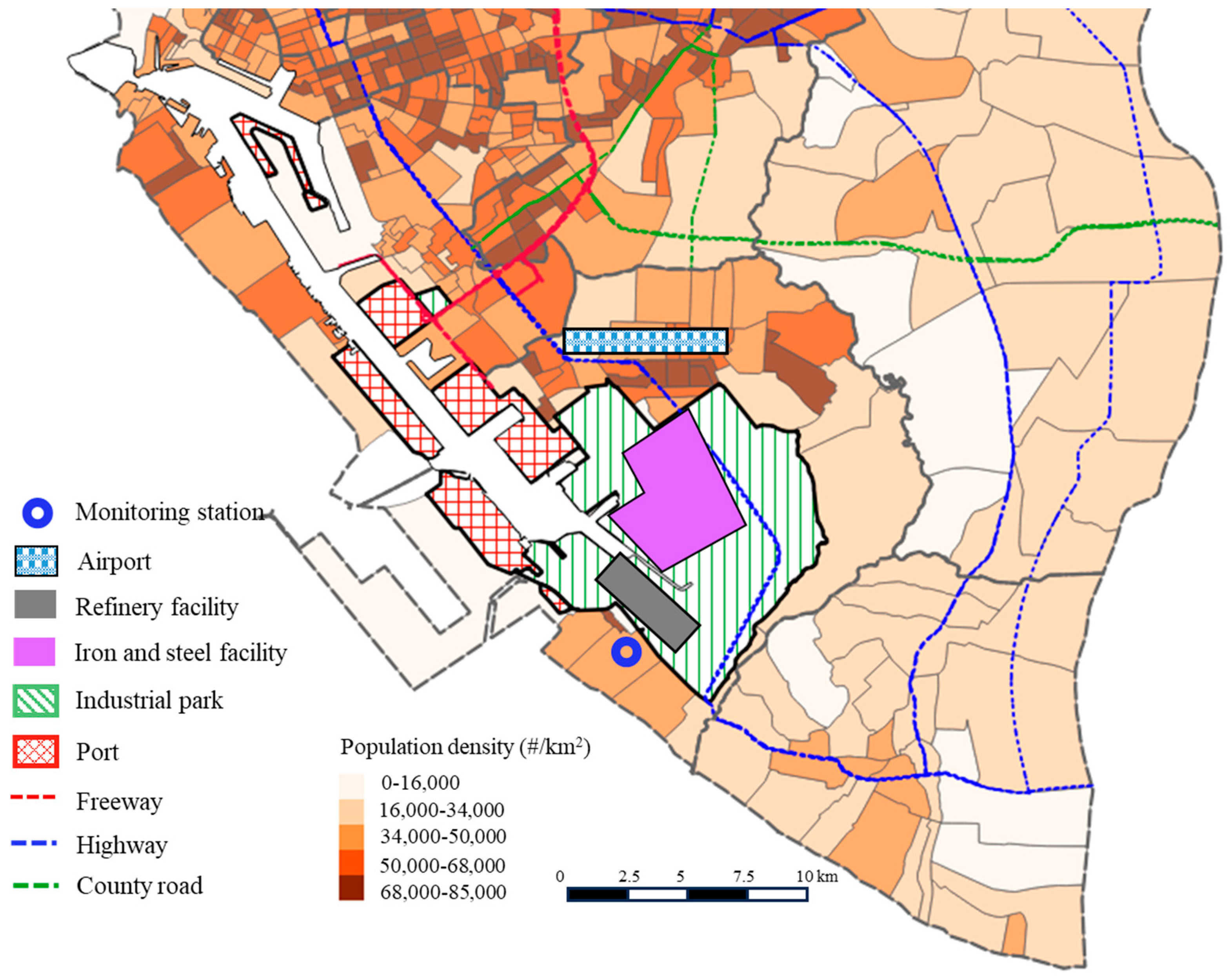
2. Materials and Methods

The Coastal Industrial Park (formerly the Coastal Industrial Zone) is located in Kaohsiung City, with Kaohsiung Port to the south, Kaohsiung International Airport approximately 500 m to the north, and the highway terminal interchange approximately 3 km to the north, making it an ideal location for industrial operations (Figure 1). Established in 1960 and developed by 1977, the park is managed by the Industrial Park Administration under the Ministry of Economic Affairs. Spanning 1560 hectares, it generates an annual production value of TWD 853.2 billion and employs 36,120 people, making it one of the largest industrial zones in Taiwan. The park hosts 501 companies, representing more than 30 industries; the park’s primary sectors are metal product manufacturing (119 companies), machinery equipment manufacturing and repair (62 companies), and basic metal manufacturing (35 companies). This park is a crucial pillar of Taiwan’s economic development and a significant hub for industrial and commercial activities. The population of the surrounding area is approximately 155,000, with 22 schools within the district.

2.1. Method for Estimating HAP Emissions

This study used 2022 as the base year. Based on toxicity, the target species were benzene, formaldehyde, 1,3-butadiene, vinyl chloride, arsenic, and DPM. The emissions from stationary sources, mobile sources, and port activities were then estimated.

2.1.1. Estimation of HAP Emissions from Stationary Sources

• Estimation of heavy metal emissions

The Ministry of Environment has been collecting air pollution fees for particulate heavy metals and persistent organic pollutants since 2018 for substances such as arsenic, cadmium, lead, mercury, hexavalent chromium, and dioxins. For 2022, the annual emissions from coastal industrial facilities were calculated by summing the quarterly reported air pollution emissions fees. Additionally, this study referenced the Ministry of Environment’s Stationary Pollution Source Management Information Disclosure Platform [14] to allocate emissions across all pipelines and relevant pollution sources within factories.

• Estimation of VOC emissions

The Ministry of Environment has been collecting air pollution fees for VOCs since 1996. According to “Stationary Pollution Source Air Pollution Fee Charges”, 13 additional harmful VOC air pollution fees have been levied since 1999, including fees for toluene, xylene, benzene, ethylbenzene, styrene, methylene chloride, 1,1-dichloroethane, 1,2-dichloroethane, chloroform, 1,1,1-trichloroethane, tetrachloroethane chlorinated carbon, trichloroethylene, and tetrachlorethylene. In 2024, fees for three hazardous VOCs—vinyl chloride, 1,3-butadiene, and acrylonitrile—were also imposed in Taiwan.

This study was based on air pollution fee data. The main sources of VOCs include the manufacturing of components (such as valves, flanges, joints, compressors, and pumps for petrochemical facilities), cooling water towers, maintenance, loading, wastewater and oil–water separation tanks, exhaust gas combustion towers, storage tank emissions, etc. Benzene emissions were calculated based on air pollution emission fee data for each process in each factory. The remaining species (formaldehyde, 1,3-butadiene, and vinyl chloride) were not subject to an additional air pollution fee, and SPECIATE emission factor data announced by the US Environmental Protection Agency were used [15]. The library ratio SPECIATE map coding was referenced from the Ministry of Environmental Protection (2020) [16]. Based on air pollution fee declaration information and stationary-pollution-source permit information, the processes were classified according to the source classification codes (SCCs), and then the SCC-Profile Cross-Reference Table provided by the US EPA website was adopted. The spectrum numbers were input into the SPECIATE database to obtain target-species proportion coefficients and to calculate the emissions of formaldehyde, 1,3-butadiene, and vinyl chloride for each process at each factory.

2.1.2. Estimation of HAP Emissions from Mobile Sources

Parameters such as the number of vehicles and sales, the usage of gasoline and diesel, cumulative vehicle mileage, fuel efficiency, etc., were collected, and the fuel consumption method was used to estimate the mileage of motor vehicles and the activity intensity for different vehicle types during each period; the emission factor was simulated using MOVES.

• Mobile-source activity intensity

The calculation of mobile-source activity intensity was divided into three steps: estimation of motor vehicles’ total mileage, construction of a road activity grid, and analysis of the activity intensity for different vehicle types during each period.

• Estimation of the total mileage from motor vehicles

We referred to the Taiwan Emission Data System version 12.0 (TEDS 12.0)-line source estimation manual [17] to calculate the total mileage of motor vehicles, and used the fuel consumption method to estimate vehicle mileage. The vehicle mileage estimation was based on vehicle fuel consumption. We used the Energy Balance Sheet published by the Energy Bureau of the Ministry of Economic Affairs to determine the total fuel consumption of vehicles nationwide [18]. We then obtained the annual sales volumes of gas stations for each county and city, based on the Monthly Statistics of Gasoline and Diesel Sales at Gas Stations in Counties and Cities from the Energy Bureau of the Ministry of Economic Affairs, and added them up to obtain the national gas station (gasoline and diesel) annual total sales volume [19]. We divided the national current energy consumption calculated in the energy balance sheet by the total annual sales volume of gas stations (gasoline and diesel) nationwide, to obtain a conversion ratio. We multiplied this ratio by the sales volume of gas stations in each county and city, to obtain the energy consumption distribution in each county and city.

• Average annual fuel consumption of each vehicle type

We referred to the TEDS12.0-line source estimation manual for the average annual mileage and fuel efficiency of different vehicle types. By dividing the two, the average annual fuel consumption of a single vehicle for each vehicle type in each county and city could be obtained. The formula is as follows:

$${\left(\mathrm{A}\mathrm{v}\mathrm{e}\mathrm{r}\mathrm{a}\mathrm{g}\mathrm{e}\mathrm{a}\mathrm{n}\mathrm{n}\mathrm{u}\mathrm{a}\mathrm{l}\mathrm{f}\mathrm{u}\mathrm{e}\mathrm{l}\mathrm{c}\mathrm{o}\mathrm{n}\mathrm{s}\mathrm{u}\mathrm{m}\mathrm{p}\mathrm{t}\mathrm{i}\mathrm{o}\mathrm{n}\right)}_{ji}={\displaystyle \frac{{\left(\mathrm{A}\mathrm{v}\mathrm{e}\mathrm{r}\mathrm{a}\mathrm{g}\mathrm{e}\mathrm{a}\mathrm{n}\mathrm{n}\mathrm{u}\mathrm{a}\mathrm{l}\mathrm{m}\mathrm{i}\mathrm{l}\mathrm{e}\mathrm{a}\mathrm{g}\mathrm{e}\right)}_{ji}}{{\left(\mathrm{A}\mathrm{v}\mathrm{e}\mathrm{r}\mathrm{a}\mathrm{g}\mathrm{e}\mathrm{f}\mathrm{u}\mathrm{e}\mathrm{l}\mathrm{c}\mathrm{o}\mathrm{n}\mathrm{s}\mathrm{u}\mathrm{m}\mathrm{p}\mathrm{t}\mathrm{i}\mathrm{o}\mathrm{n}\mathrm{v}\mathrm{a}\mathrm{l}\mathrm{u}\mathrm{e}\right)}_{ji}}}$$

(1)

where i is the vehicle type and j is the fuel type.

• Average annual fuel consumption ratio of gasoline/diesel vehicles

We used the average annual fuel consumption of each vehicle type and multiplied it by the number of motor vehicle registrations on the Statistical Inquiry Network of the Highway Administration of the Ministry of Transport to screen the number of each vehicle type in different counties and cities, to obtain the total annual fuel consumption for different vehicle types in each county and city. The formula is as follows [20]:

$$\begin{gathered} AverageAnnualFuelConsumptionRatiosbyVehicleTypeforGasoline/Diesel \\ ={\displaystyle \frac{{AverageAnnualFuelConsumption}_{ji}\times {NumberofVehiclesinUse}_{ji}}{{\sum AverageAnnualFuelConsumption}_{ji}\times {NumberofVehiclesinUse}_{ji}}} \end{gathered}$$

(2)

• Total vehicle mileage traveled on different roads in different years

The calculated annual total vehicle mileage of different vehicle types in each county and city was compiled, according to the experience ratio of each road category allocation made by this research office. The annual total vehicle mileage of different vehicle types was allocated to different road types (divided into freeway, highway, county roads, and urban roads); that is, the total annual vehicle mileage of each vehicle type and road in each county and city was obtained.

• Average annual mileage of each vehicle age

Based on the Ministry of Transport’s survey report for use of gasoline passenger cars, commercial gasoline passenger cars, motorcycles, and tour buses, mileage (km) data corresponding to each vehicle’s age was collected. Using exponentiation, logarithmic regression analysis, and polynomials, the average annual mileage with the higher R² was selected as the recommendation, and a cumulative mileage distribution corresponding to each vehicle age was drawn up. The accumulated mileage of each vehicle age was subtracted from the accumulated mileage for the previous year to obtain the mileage of a vehicle of that age. If there were no survey report for other vehicle types, the average annual mileage data of each vehicle type in TEDS12.0 were used to estimate the proportion.

• Estimation of the activity intensity for each vehicle type during different periods

We used the number of vehicles registered by the Ministry of Transportation and Communications and selected vehicle age categories to obtain the number of vehicles of different vehicle types and ages. Next, we multiplied these results by the average annual mileage of each vehicle type and age, to obtain the activity intensities for each vehicle type and age. We then divided these results by the sum of the activity intensity of each vehicle type and age, to obtain the activity intensity ratios. Finally, the activity intensity ratios of each vehicle age group were added up to obtain the activity intensity ratios of each vehicle type during different periods. Subsequently, the emissions of each vehicle type could be calculated in different periods. The formula is as follows:

$$S_i={\displaystyle \frac{Y_i\times D_i}{{\sum }_{i=1}^{i=25}{Y}_i\times D_i}}$$

(3)

where S_i is the vehicle activity intensity in the base year when the vehicle age is the i-th year; Y_i is the number of vehicles whose age is the i-th year in the base year; and D_i is the average annual mileage of vehicles whose age is the i-th year in the base year.

• Mobile-source emission factor

This study divided estimated HAP emission factors into two categories: volatile and particulate air pollutants. For volatile HAPs, refer to Liu (2018) [21]. For motorcycles and gasoline vehicles, benzene, and formaldehyde, a dynamometer test was used to establish the emission factor and fingerprint data of volatile HAPs. For 1,3-butadiene, there were no dynamometer test data. We referred to the TEDS12.0 HC exhaust emission factors of various vehicle types, which correspond to the SPECIATE 5.1 fingerprint database. To calculate the emission factors for diesel vehicles, we referred to the TEDS12.0 HC exhaust emission factor of each vehicle type for benzene, formaldehyde, and 1,3-butadiene. For HAPs in PM, arsenic and DPM, emission factors were obtained using the laboratory’s collection of PM data and a MOVES simulation.

• Construction of road-grid activity intensity

This study used the Quantum Geographic Information System (QGIS) tool to establish a 200 × 200 m road grid within the study area, including freeways, highways, county roads, and township and urban roads. The freeways and highways were matched with a numerical road network map based on traffic volume data from the Ministry of Transport, in which each road section has a corresponding traffic volume. The road length of this section was multiplied by the traffic volume, to obtain the section’s mileage. County roads and township/city roads were relatively complicated. We mainly referenced the traffic flow survey data of important roads adjacent to the port area of the Transportation Research Institute of the Ministry of Transport (2021) [22] and matched the traffic flow data with the numerical road network map. The remaining roads were aggregated by vehicle type. After deducting the vehicle mileage from national and provincial highways, the total vehicle mileage was estimated using the fuel consumption method, and distributed to each road grid in proportion to the road level.

2.1.3. Estimation of HAP Emissions from Port Activities

Based on the port inventory data from the Ministry of Environment, data on the emissions of VOCs (benzene, formaldehyde, 1,3-butadiene, and vinyl chloride), PM (arsenic), and DPM were collected; these emission factors corresponded to those of HAP pollution sources from the US Environmental Protection Agency SPECIATE.

Referring to the “Port Emission Inventory” of the Ministry of Environmental Protection [23] and emission estimation research for port areas such as San Pedro Bay Ports in California [24], the emission sources for port activities include ocean-going vessels, ships and fishing vessels operating in the port area, cargo handling equipment, and heavy-duty vehicles. We collected data on the VOC and PM emissions from individual sources at the port (water areas within the port administrative area) and referred to the SPECIATE fingerprint database to estimate various emissions based on the basic characteristics of the emission sources corresponding to the fingerprint data, targeting HAP (benzene, formaldehyde, 1,3-butadiene, arsenic, and DPM) emissions.

2.2. Carcinogenic Weight of Emission Characteristics

Referring to the MATES V emission carcinogenic weight method, each emission type was multiplied by the carcinogenic slope factor (

Table 1. Carcinogenicity toxicity factors for hazardous air pollutants.

#	CAS No.	Name	Classification 1	ICPF 2 (mg/kg/day)−1
1	7440-38-2	arsenic	1	1.2 × 101
2	--	DPM	1	1.1
3	71-43-2	benzene	1	1.0 × 10−1
4	50-00-0	formaldehyde	1	2.1 × 10−2
5	106-99-0	1,3-butadiene	1	0.6
6	75-01-4	vinyl chloride	1	0.3

Notes: ¹ Classification by IARC: “1”, carcinogenic to humans; ² ICPF: inhalation cancer potency factor, #: number. Source: Consolidated Table of OEHHA/CARB Approved Risk Assessment Health Values (2020) https://ww2.arb.ca.gov/resources/documents/consolidated-table-oehha-carb-approved-risk-assessment-health-values (accessed on 12 June 2023).

) and converted into a percentage, which was also the carcinogenic weight of that emission, to evaluate the regulatory priority of each species’ composite source emissions.

2.3. Model Performance Evaluation and Correction

We referred to the AERMOD model manual [25] and used the Rankfile results to draw quantile–quantile plots (QQ plot) to compare differences between the monitored data and the simulated data. When the data fell on a straight line with a slope of 1:1, the monitored data were similar to the simulation data. When the data fell on a line with a slope of below 1:1, the simulated data were lower than the measured data, and the simulation result was an underestimate. When the data points fell on a line with a slope above 1:1, the simulated data were higher than the measured data, and the simulation result was an overestimate.

As all emission sources in the study area were not considered, to understand the differences between the simulation results and the monitored concentrations, the least squares method was used to evaluate whether the simulation results needed to be adjusted using correction factors. The least squares method formula is as follows:

$$e=\sqrt{{\displaystyle \frac{({C_1-M_1)}^2+({C_2-M_2)}^2+\dots ({C_i-M_i)}^2}{i}}}$$

(4)

where e is error; C_i is the i-th original simulated concentration; and M_i is the i-th multiple of the simulated concentration.

2.4. Simulation Analysis of HAP Concentration

We referred to the AERMOD model simulation manual of the Air Quality Model Support Center of the Ministry of Environment as a diffusion concentration simulation tool, as well as meteorological data and terrain data from the Ministry of Environment; the grid resolution was set to 200 m × 200 m. We integrated the emission parameters required for an AERMOD model stationary source pipeline simulation, including the pollutant emission rate (g/s), chimney height (m), exhaust temperature (K), chimney outlet exhaust rate (m/s), discharge port inner diameter (m), and other parameters. Mobile source simulations used a body source, and simulation settings included the emission rate (g/s) and the emission height above the ground (m). The national and provincial highway bridge height was set at about 10 m, and the emission height of county and urban roads was set at about 0.3 m. The port area was simulated using area sources, which were divided into land and sea areas. Ship emissions were allocated to the sea area, and vehicles and loading and unloading equipment were allocated to the land area (shown in

Table 2. AERMOD mode parameter-setting values.

Simulation Settings	Parameter
Area	Industrial complex, port, and adjacent extended areas
Topography	Complex
Scope	15 km × 15 km
Coordinates	Starting point: (173,400, 2,488,600); Endpoint; (188,400, 2,503,600)
Species	Benzene, formaldehyde, 1,3-butadiene, vinyl chloride, arsenic, DPM
Source type	Stationary source (pipeline): point source; fixed source (escape): area source; mobile source: Ti source; port activities: area source
Emission-source height	Stationary source: pipeline (input based on height of each chimney), escape (0.5 m); mobile source: 10 m for national roads, 0.3 m for provincial, county, and city roads; port activities: 25 m for ships, 39 m for handling equipment, 0.3 m for vehicles
Grid resolution	200 m × 200 m
Meteorological data	Surface	Kaohsiung station
	Profile	Pingtung station
Simulation year	2022
Notes	Used metropolitan area parameters and did not consider smoke downwash Used AERMOD main program, version 21112

). Referring to Kotrikla et al. (2013) [26], we assumed that the ship emission height was 25 m, and the estimated simulation emission grid size was 200 m × 200 m. Each target species was simulated, and the data are presented in terms of average annual incremental concentration (background concentrations of the atmosphere are not included). Regarding the MATES V report, the simulated concentration characteristics of individual pollutants are discussed separately, without considering the synergistic effects between species.

The AERMOD-stimulated concentrations were compared with ambient air monitoring data. In addition, the average incremental concentrations of each composite source in the grid were compared with the international environmental concentration reference data from air quality guidelines of World Health Organization (WHO) [27], the air monitoring comparison values of the Texas Commission on Environmental Quality (TCEQ) [28], and the environmental standards and guideline values of the Ministry of Environment of Japan [29].

2.5. Environmental Impact Assessment

Referring to the OEHHA risk assessment guidelines, the model simulated the average annual concentrations, to estimate the risk of cancer caused by inhaling pollutants. The USEPA considers a carcinogenic risk between 10⁻⁴ and 10⁻⁶ to be an acceptable value, with a risk value > 10⁻⁴ as the boundary. Control measures should be taken when exceeding this boundary.

3. Results and Discussion

3.1. Emission Characteristics of Composite Emission Sources

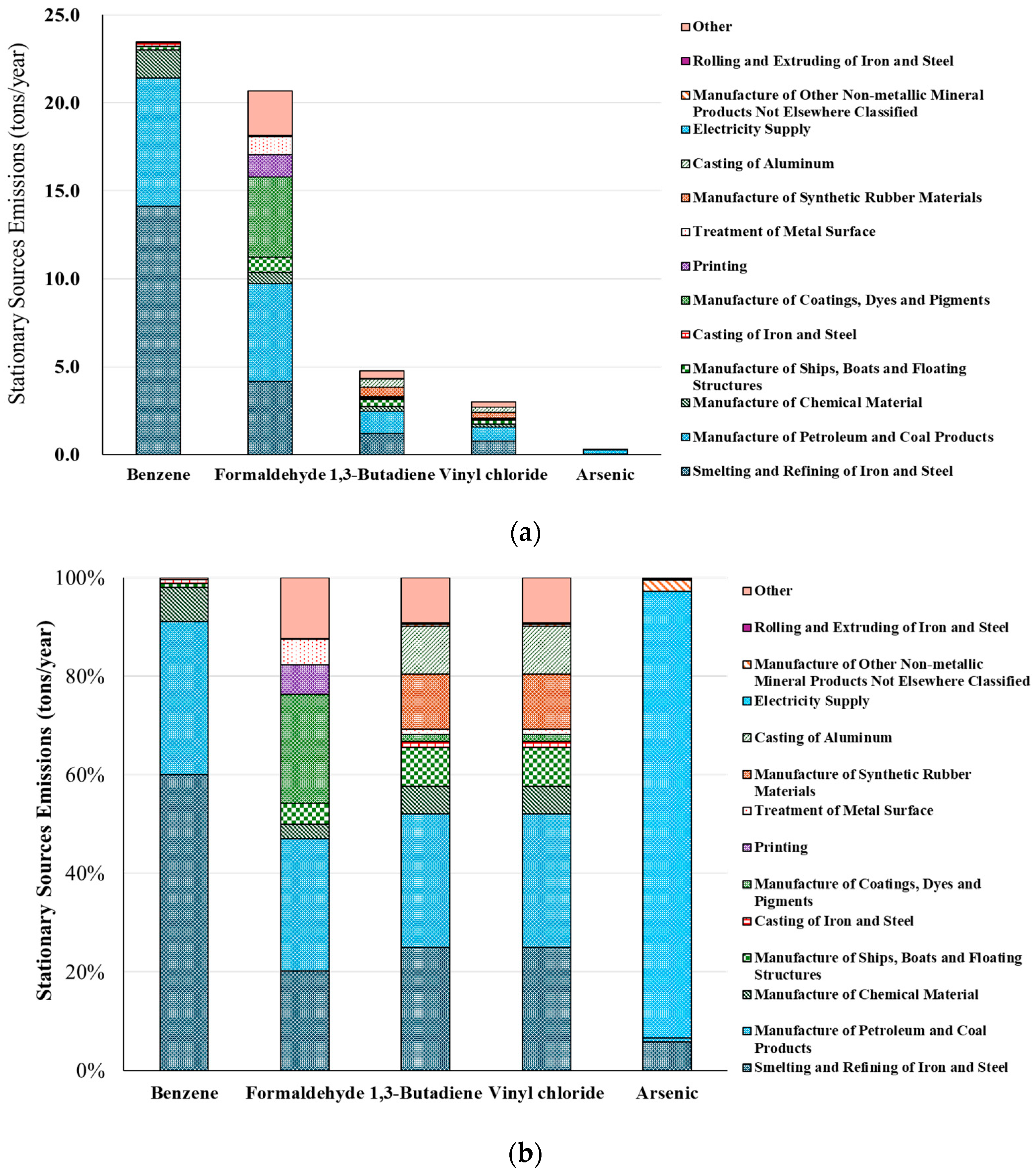
3.1.1. Stationary-Source Emission Characteristics

The HAPs emitted from stationary sources were mainly benzene, formaldehyde, 1,3-butadiene, vinyl chloride, and arsenic. Their emission results are shown in Figure 2a, and their emission proportion results in Figure 2b; the emission amounts and proportions of these five pollutants can be ranked in the following order: benzene (23.5 ton, 45%) > formaldehyde (20.7 ton, 40%) > 1,3-butadiene (4.7 ton, 9%) > vinyl chloride (3.0 ton, 6%) > arsenic (267.2 kg, 1%).

Their carcinogenic weights were 33% for arsenic, 30% for 1,3-butadiene, 24% for benzene, 8% for vinyl chloride, and 5% for formaldehyde. Based on industry-specific carcinogenic weights, benzene was mostly emitted by the steel smelting chain industry (15%) and the petroleum and coal products manufacturing industry (8%); formaldehyde was emitted by the petroleum and coal products manufacturing industry (1%) and from the manufacturing of coatings, dyes, and pigments (1%); 1,3-butadiene was mostly emitted by the petroleum and coal products manufacturing industry (8%) and the steel smelting chain industry (7%); vinyl chloride was also generated by the petroleum and coal products manufacturing industry (7%); and arsenic was emitted by the manufacturing industry (2%), the steel smelting chain industry (2%), the power supply industry (30%), and the steel smelting chain industry (2%) (as shown in

Table 3. Carcinogenic weights of stationary-source emissions (%).

Type	Benzene	Formaldehyde	1,3-Butadiene	Vinyl Chloride	Arsenic	Total
Smelting and refining iron and steel	15	1	7	2	2	27
Manufacture of petroleum and coal products	8	1	8	2	0	19
Manufacture of chemical material	2	0	2	0	0	4
Manufacture of ships, boats, and floating structures	0	0	2	1	--	3
Casting iron and steel	0	0	0	0	0	1
Manufacture of coatings, dyes, and pigments	0	1	0	0	--	2
Printing	--	0	--	--	--	0
Treatment of metal surfaces	--	0	0	0	--	1
Manufacture of synthetic rubber materials	--	0	3	1	--	4
Casting aluminum	--	0	3	1	--	4
Electricity supply	--	0	--	--	30	30
Manufacture of other non-metallic mineral products not elsewhere classified	--	0	0	0	1	1
Rolling and extruding iron and steel	--	0	0	0	0	0
Other	0	1	3	1	0	4
Total stationary sources	24	5	30	8	33	100

Note: -- means no emissions.

).

3.1.2. Mobile Sources

Mobile sources primarily emitted benzene, formaldehyde, 1,3-butadiene, arsenic, and DPM. The emission results are shown in Figure 3a, and the emission proportion results are shown in Figure 3b; the emission amounts and proportions of these five pollutants can be ranked in the following order: DPM (6.6 ton, 55%) > benzene (2.7 ton, 23%) > 1,3-butadiene (1.5 ton, 12%) > formaldehyde (1.1 ton, 10%) > arsenic (1.1 kg, <1%).

The carcinogenic weights were 86% for DPM, 10% for 1,3-butadiene, 3% for benzene, <1% for formaldehyde, and <1% for arsenic. An analysis of the carcinogenic weight of each vehicle type attributed the emission of DPM largely to diesel vehicles (86%); the carcinogenic weight of diesel pickup trucks was 50%. The emission of 1,3-butadiene was mostly caused by locomotives (7%); the carcinogenic weight ratio of four-stroke motorcycles was close to 100%. Benzene was mainly emitted by gasoline vehicles (2%); the carcinogenic weight ratio of self-use gasoline passenger cars was 98%. Formaldehyde was primarily emitted by gasoline vehicles (<1%). Arsenic was mainly emitted by gasoline vehicles (<1%); the carcinogenic weight of self-use gasoline passenger cars was 94% (as shown in

Table 4. Carcinogenic weights of mobile-source emissions (%).

Type	Benzene	Formaldehyde	1,3-Butadiene	Arsenic	DPM	Total
Gasoline vehicles	2	0	3	0	--	5
Diesel vehicles	0	0	0	0	86	87
Motorcycles	1	0	7	0	--	8
Other	0	0	0	0	--	0
Total mobile sources	3	0	10	0	86	100

Note: -- means no emissions.

).

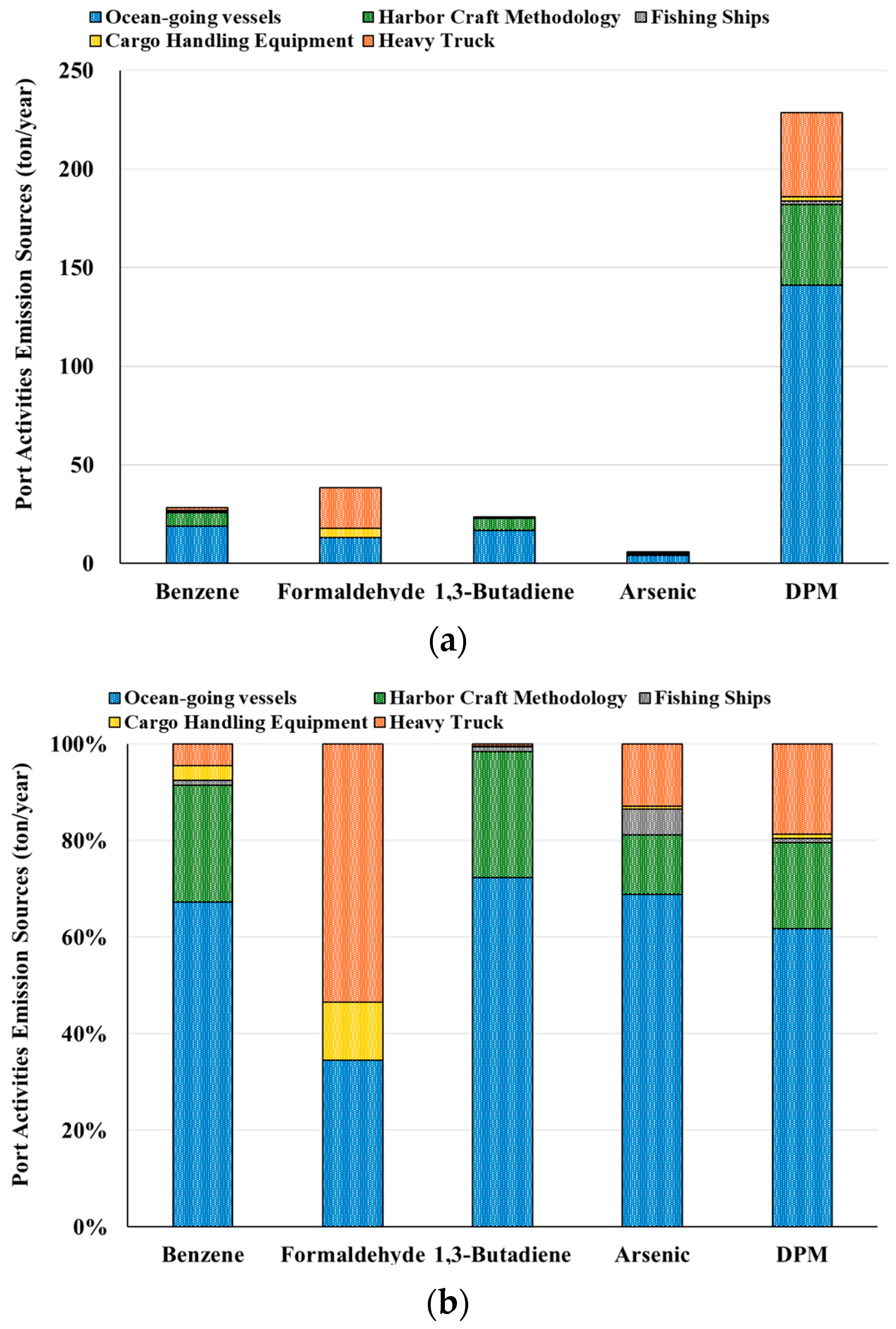
3.1.3. Port Activities

The main pollutants emitted from port area activities were benzene, formaldehyde, 1,3-butadiene, arsenic, and DPM. The emission results are shown in Figure 4a, and the emission proportion results are shown in Figure 4b; the emissions of these five pollutant species can be ranked in the following order: DPM (228.6 ton, 72%) > formaldehyde (38.3 ton, 12%) > benzene (28.1 ton, 9%) > 1,3-butadiene (23.1 ton, 7%) > arsenic (5.8 kg, <1%).

Their carcinogenic weights were 93% for DPM, 5% for 1,3-butadiene, 1% for benzene, <1% for formaldehyde, and <1% for arsenic. DPM was emitted by ocean-going vessels (60%); 1,3-butadiene was emitted by ocean-going vessels (4%); benzene was emitted by ocean-going vessels (1%); and formaldehyde was emitted by heavy-duty vehicles (<1%) (as shown in

Table 5. Carcinogenic weights of port activity source emissions (%).

Type	Benzene	Formaldehyde	1,3-Butadiene	Arsenic	DPM	Total
Ocean-going vessels	1	0	4	0.0	58	62
Harbor craft methodology	0	--	1	0.0	17	18
Fishing ships	0	--	0	0.0	1	1
Cargo handling equipment	0	0	0	0.0	1	1
Heavy trucks	0	0	0	0.0	18	18
Total	1	0	5	0.0	93	100

Note: -- means no emissions.

).

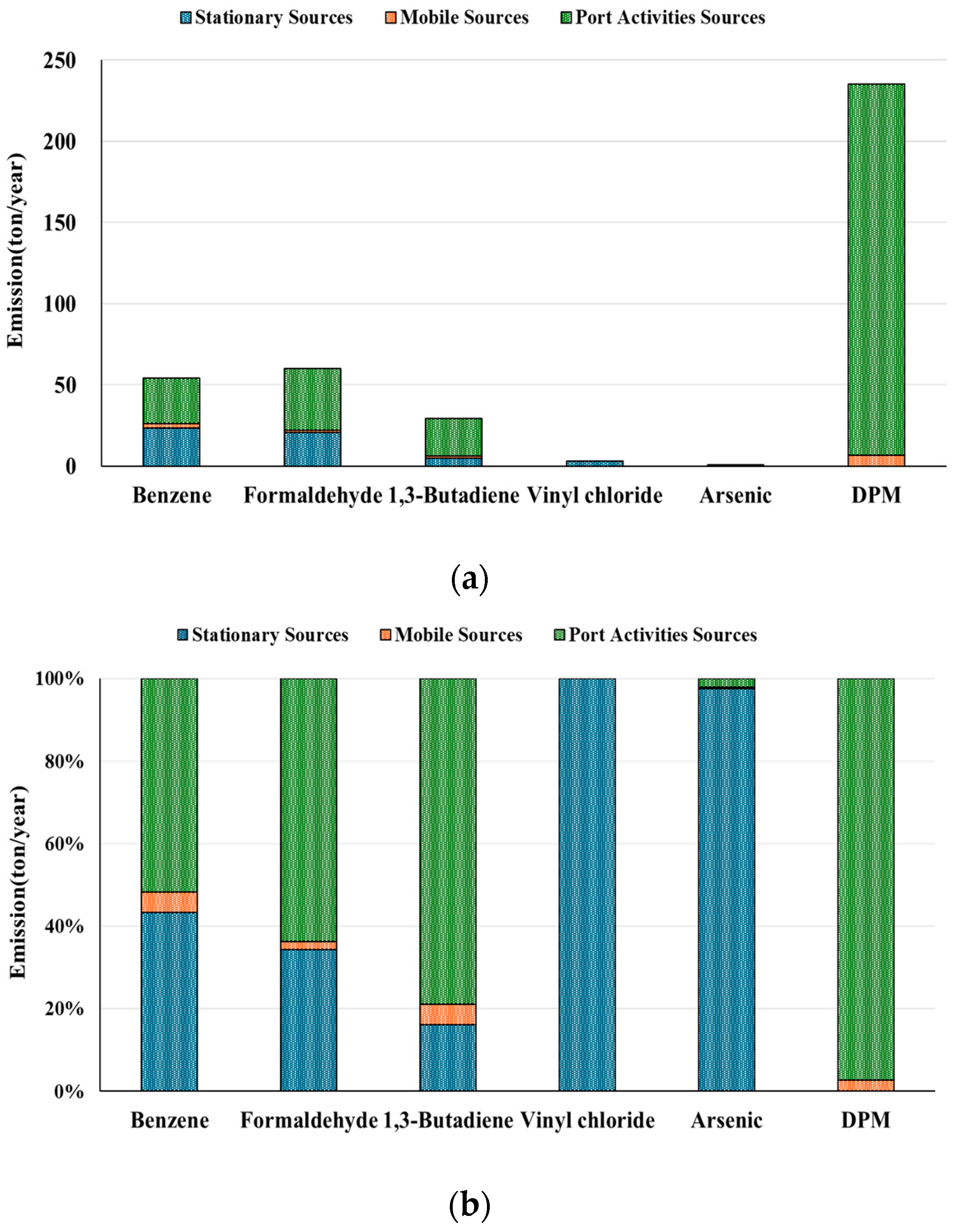
3.1.4. Composite Sources

The baseline scenario emissions and carcinogenic potentials of the three types of emission sources are shown in Figure 5a, and the emissions proportion results are shown in Figure 5b; the order of emissions from composite sources is DPM (235.2 ton) > formaldehyde (60.2 ton) > benzene (54.3 ton) > 1,3-butadiene (29.3 ton) > vinyl chloride (3.0 ton) > arsenic (0.3 ton). DPM was caused by ocean-going vessels operating in the port area (141.1 ton), heavy-vehicle emissions (42.8 ton), and ships operating in the port area (40.9 ton); formaldehyde was generated by emissions from heavy-duty vehicles (20.5 ton) active in the port area.

The carcinogenic weights of composite source emissions can be ranked in the following order: DPM (90%) > 1,3-butadiene (6%) > benzene (2%) > arsenic (1%) > formaldehyde (<1%) > vinyl chloride (<1%). The primary sources of DPM emission included ocean-going vessels (54%), heavy-duty vehicles (16%), and port operation ships (16%); 1,3-butadiene was from ocean-going vessels (4%) (as shown in

Table 6. Carcinogenic weights of composite source emissions (%).

Sources	Benzene	Formaldehyde	1,3-Butadiene	Vinyl Chloride	Arsenic	DPM	Total
Stationary	1	0	1	0	1	--	3
Mobile	0	0	0	--	0	3	3
Port Activities	1	0	5	--	0	88	94
Total	2	0	6	0	1	91	100

Note: -- means no emissions.

).

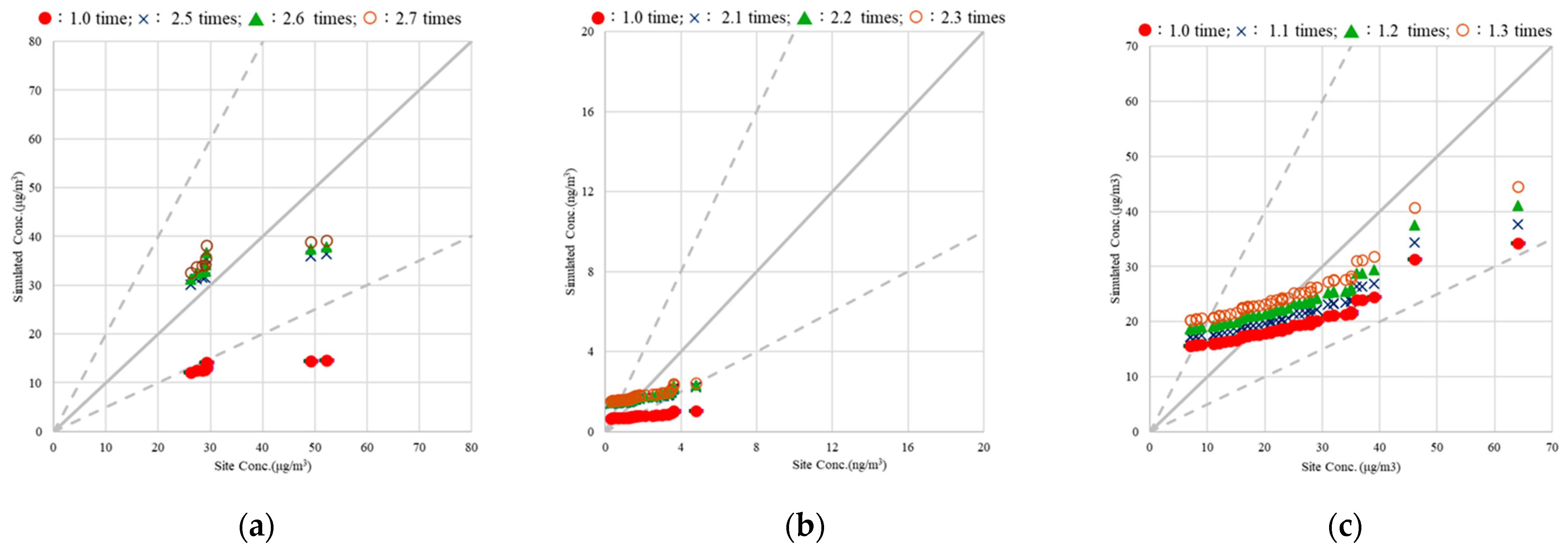
3.2. Emission Calibration

3.2.1. Performance Verification Evaluation

This study considered the degree of hazard at the monitoring station due to emissions from composite sources, and compared the meteorological data selected from individual monitoring stations and models. Based on the data, monitoring station A, which was located downwind of the industrial park and the port, was selected for performance verification.

1.

Benzene

The monitored data and simulated benzene concentration data were close to the 1:1 slope, indicating that the monitoring data were similar to the simulated data. The model’s performance was evaluated using statistical methods. The results showed that the normalized mean square errors (NMSEs) were 0.1, the fractional bias (FB) was −0.1, the Fa2 (fraction of predictions within a factor of two of observations) was 1.1, and the correlation coefficient (R) was 0.9, implying the performance verification results are good.

2.

Formaldehyde

The simulation result was located below the slope line, which means that the simulation data were lower than the monitoring data. This suggests the simulation result was an underestimation. The model’s performance was evaluated using statistical methods. The results show that the NMSEs were much greater than 0.5, the FB was 0.9, the Fa2 was 0.4, and the R was 0.7, indicating poor validation results.

In addition, relevant plans for special industrial zones noted that the monitoring station analyzed the levels of formaldehyde using an absorption method. Compared with other methods, the absorption method leads to the detection of higher concentrations of formaldehyde. This may be one of the reasons for the poor performance verification. However, the method for analyzing the levels of formaldehyde resulted in higher results, leading to an underestimation of emissions.

3.

Arsenic

The simulation result was located below the slope line, which means that the simulation data were lower than the monitoring data. This implies that the simulation result was an underestimation. The model’s performance was examined using statistical methods. The results show that the NMSEs were 0.3, the FB was 0.7, the Fa2 was 0.5, and the R was 0.9, indicating poor performance verification results. This study used data from specialized industrial areas. As new arsenic-monitoring data points are obtained from manual sampling every six days, they could not be used to completely test the performance of the AERMOD model.

4.

DPM

The simulation results and monitoring-station concentration results were distributed above and below the slope line, which means the simulation data were lower than the monitoring data. This indicates that these simulation results were an underestimation. The model’s performance was analyzed using statistical methods. The results show that the NMSEs were 10.5, the FB was 0.2, the Fa2 was 0.8, and the R was 0.9, suggesting poor performance verification results. The mobile source emissions were determined for DPM; however, some diesel engines and boilers used were not included in the emissions determination.

The above results confirmed that the performance verification results for benzene were good and that the other species’ simulated concentrations were low. There are three reasons for this. First, regarding the special industrial area data used in this study, only benzene’s data were obtained by monitoring stations automatically as hourly data. Other species were monitored by manual stations (data every 6 days); therefore, no daily average concentrations were available for these other species. Second, for the stationary sources, air pollution emissions fees were reported for benzene and arsenic species, but for other species, the declared VOC quantities were multiplied by the foreign SPECIATE 5.1 emission factor, causing overestimation/underestimation of the calculation results. Third, only industrial parks, traffic roads, port ships, machinery and equipment, etc., were considered pollution sources in the simulation. However, to make the model’s simulation results more accurate, other emission sources (gas stations, agricultural machinery and equipment, and fugitive source emissions) need to be considered. Inputting more pollution sources will lead to an increase in variables, and the simulation results may not be more accurate. Therefore, the monitoring data from special industrial areas were used as the benchmark for performance verification.

3.2.2. Emission Corrections

1.

Formaldehyde

The results are shown in Figure 6a. The minimum variance at a correction multiple of 1.0 time is 22.5, and the minimum variance at a correction multiple of 2.6 times is 8.003. Therefore, the minimum variance is at a correction multiple of 2.6 times.

2.

Arsenic

The results are shown in Figure 6b. The minimum variance at a correction multiple of 1.0 time is 1.2, and the minimum variance at a correction multiple of 2.2 times is 0.797. Therefore, the minimum variance is at a correction multiple of 2.2 times.

3.

DPM

The results are shown in Figure 6c. The minimum variance at a correction multiple of 1.0 times is 9.6, and the minimum variance at a correction multiple of 1.3 times is 8.094. Therefore, the minimum variance is at a correction multiple of 1.3 times.

3.3. Analysis of Simulated HAPs

The model-simulated concentration spatial distribution results are shown in Figure 7.

1.

Benzene

The average incremental concentration for benzene was 1.9 μg/m³, and the maximum was 140.5 μg/m³. The average and maximum were both caused by stationary-source emissions. Comparing the average incremental concentration of benzene with the WHO environmental reference standard (0.5 ppb/1.7 μg/m³) [27], this composite emission source was 1.1 times the limit. In terms of stationary sources, benzene mainly came from industrial parks; in terms of mobile sources, urban roads; and in terms of port activities, ocean-going vessels, spreading from the port area to the periphery.

2.

Formaldehyde

The average incremental concentration for formaldehyde was 7.6 μg/m³, and the maximum was 238.6 μg/m³. The average was the result of emissions from port activities. The maximum was due to emissions from stationary sources. Comparing the average for formaldehyde with the TCEQ environmental reference standard (8.9 ppb/10.9 μg/m³) [28], this composite emission source was 0.7 times the limit. In terms of stationary sources, formaldehyde primarily came from industrial parks; in terms of mobile sources, urban roads; and in terms of port activities, heavy vehicles and ocean-going vessels, spreading from the port area to the periphery.

3.

1,3-Butadiene

The average and maximum incremental concentrations for 1,3-butadiene were 0.5 μg/m³ and 29.3 μg/m³, respectively. The average was mainly affected by emissions from port activities, and the maximum was mainly affected by emissions from stationary sources. The average for 1,3-butadiene was compared with the Japanese environmental reference standard (1.1 ppb/2.5 μg/m³) [29], and this composite emission source was 0.2 times the limit. In terms of stationary sources, 1,3-butadiene primarily came from industrial parks; in terms of mobile sources, urban roads; and in terms of port activities, ocean-going vessels, spreading from the port area to the periphery.

4.

Vinyl chloride

The average and maximum incremental concentrations for vinyl chloride were 0.1 μg/m³ and 18.0 μg/m³, respectively. Comparing the average with the Japanese environmental reference standard (3.9 ppb/10.0 μg/m³) [29], this stationary source was less than 0.1 times the limit. In terms of stationary sources, vinyl chloride primarily came from industrial parks. The maximum incremental grid concentration of the stationary source was 18.0 μg/m³, with the highest value for industrial parks.

5.

Arsenic

The average and maximum incremental concentrations of arsenic were 0.7 ng/m³ and 14.8 ng/m³, respectively. Stationary source emissions caused both the average and maximum incremental concentrations. The average incremental concentration of arsenic was compared with the WHO environmental reference standard (6.6 ng/m³) [27], and this composite emission source was 0.1 times the limit. In terms of stationary sources, arsenic primarily came from industrial parks; in terms of mobile sources, urban roads; and in terms of port activities, ocean-going vessels, spreading from the port area to the periphery.

6.

DPM

The average and maximum incremental concentrations of DPM were 6.0 μg/m³ and 40.2 μg/m³, respectively. Both the average and maximum were mainly affected by port activities. In terms of mobile sources, DPM primarily came from urban roads; in terms of vehicle type, diesel vehicles; and in terms of port activities, ocean-going vessels, spreading from the port area to the periphery.

The overall research results show that only the atmospheric benzene concentration influenced by emissions from composite sources exceeded the environmental concentration limit.

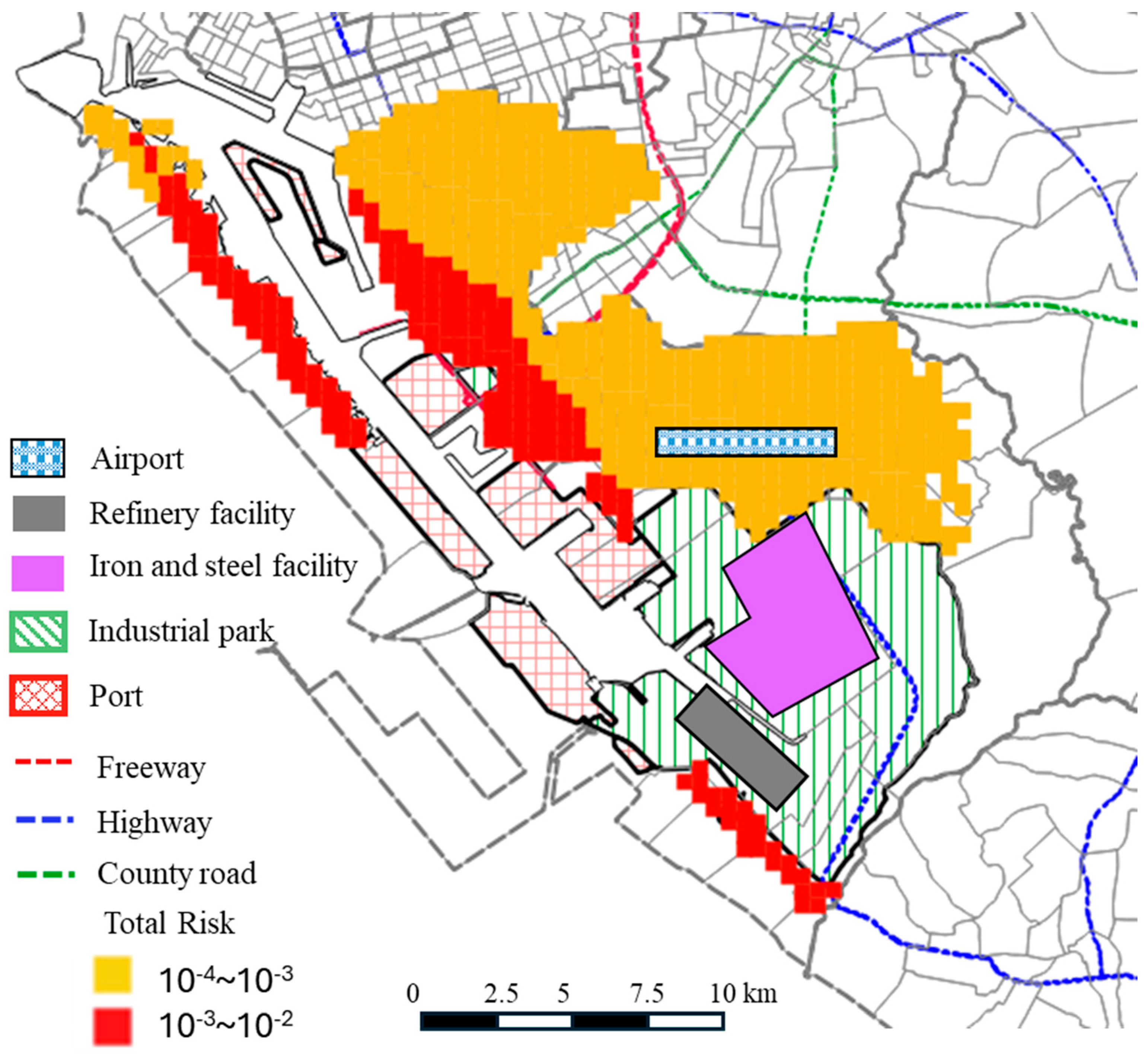
3.4. Potential Risk Assessment of Hotspots

The results for the potential risk assessment of hotspots are shown in Figure 8.

1.

Benzene

Of the densely populated areas, 1% was affected by benzene, with a risk value ranging from 10⁻³ to 10⁻⁴; 81% had risk values ranging from 10⁻⁴ to 10⁻⁵; and 18% had values ranging from 10⁻⁵ to 10⁻⁶.

2.

Formaldehyde

Of the densely populated areas, 1% was influenced by formaldehyde, with a risk value in the range of 10⁻³–10⁻⁴; 37% had risk values in the range of 10⁻⁴–10⁻⁵; and 62% had values in the range of 10⁻⁵–10⁻⁶.

3.

1,3-Butadiene

Of the densely populated areas, 2% was influenced by 1,3-butadiene, with a risk value ranging from 10⁻³ to 10⁻⁴, and 98% had risk values ranging from 10⁻⁴ to 10⁻⁵.

4.

Arsenic

Of the densely populated areas, 60% was impacted by arsenic, with a risk value ranging from 10⁻⁵ to 10⁻⁶.

5.

DPM

Of the densely populated areas, 22% was influenced by DPM, with a risk value > 10⁻³, and 78% had risk values between 10⁻³ and 10⁻⁴.

6.

Total cancer risk

The results are presented in Figure 9; 25% of the densely populated area had composite emission sources with a risk value > 10⁻³, and 75% of the area’s risk value was between 10⁻³ and 10⁻⁴.

A large integrated industrial park (where steel production, sewage treatment, natural gas-related industry, pharmaceuticals, and industrial boiler were the main emission sources of VOCs) was investigated in the upper reaches of the Yangtze River. Results showed the lifetime cancer risk values of 1,2-dibromoethane, 2-chlorotoluene, 1,3-butadiene, naphthalene, carbon tetrachloride, and bromodichloromethane were over 1 × 10⁻³, indicating that these species pose a definite carcinogenic risk and should be specially concerning [30]. In Beijing, benzene, ethylbenzene, formaldehyde and acetaldehyde were the main attributes to the carcinogenic risks. The cumulative carcinogenic risks in the industrial and urban regions were 1.95 × 10⁻⁵ and 1.21 × 10⁻⁵, respectively [31]. In addition, the carcinogenic risks of specific species (1,3-butadiene, acetaldehyde, benzene, chloroform and 1,2-dichloroethane) and the cumulative cancer risk of VOC species was 2.8–15 × 10⁻⁵ at different pollution levels in a suburban area between Beijing and Tianjin [32]. Based on the study of MATES V, the cancer risk of the air toxics at the monitoring locations ranged from 585 to 842 × 10⁻⁶. Diesel PM, benzene, 1,3-butadiene, and carbonyls are the main contributing species to cancer risk. The higher risk of cancer was located near the ports of Los Angeles and Long Beach and Los Angeles international airport [12]. In Linhai industrial park, the corresponding cancer risk could be up to 10⁻³. Formaldehyde, 1,2-dichloroethane, acetaldehyde, benzene, 1,3-butadiene and vinyl chloride are the high-risk species in urban industrial complex areas in southern Taiwan [33]. By comparing these results with those of other studies, the cumulative carcinogenic risks obtained in the industrial complex and port area (10⁻²–10⁻³) were significantly higher than in the industrial park in the vicinity of the Yangtze River [30], the industrial and urban regions of Beijing [31], and the suburban area between Beijing and Tianjin [32] in China. For the MATES V study, the lifetime cancer risk was 10⁻³–10⁻⁴, which is also lower than the cancer risk of this study [12]. Based on our previous study in the area, the risk was much lower than in this work, which could be due to exclusion of the diesel PM [33]. Most studies show that the VOCs (halogenated VOCs, carbonyls, benzene, 1,3-butadiene, etc.) were major species which cause cancer risk in rural, urban, and industrial areas.

4. Conclusions

The carcinogenic weightings for stationary source emissions were as follows: arsenic (33%), 1,3-butadiene (30%), benzene (24%), vinyl chloride (8%), and formaldehyde (5%). Arsenic emissions were primarily from the electricity supply industry (91%) and the steel smelting industry (6%). 1,3-butadiene emissions were mainly from the petroleum and coal product manufacturing industry (27%) and the steel smelting industry (25%). Benzene emissions were primarily from the steel smelting industry (60%) and the petroleum and coal product manufacturing industry (31%). The carcinogenic weightings for mobile source emissions were as follows: DPM (86%), 1,3-butadiene (10%), benzene (3%), formaldehyde (<1%), and arsenic (<1%). DPM emissions were predominantly from diesel vehicles (86%). 1,3-butadiene emissions were mainly from motorcycles (7%), whereas benzene emissions were mostly from gasoline vehicles (2%). The carcinogenic weightings for port activity were as follows: DPM (93%), 1,3-butadiene (5%), benzene (1%), formaldehyde (<1%), and arsenic (<1%). DPM emissions were largely from ocean-going vessels (60%). 1,3-butadiene emissions were primarily due to ocean-going vessels (4%), as were benzene emissions (1%). Formaldehyde emissions were heavily attributed to heavy-duty vehicles (<1%).

When the primary emission sources’ total emissions and carcinogenicity were analyzed, the results indicated that DPM posed a 90% health risk; 1,3-butadiene, 6%; benzene, 2%; arsenic, 1%; and other species, less than 1%. The carcinogenic weighting of complex-source emissions was primarily influenced by port activities, with DPM emission sources including ocean-going vessels (54%), heavy-duty vehicles (16%), and port operational vessels (16%). 1,3-butadiene emissions were primarily due to ocean-going vessels (4%). High DPM emissions occurred around the port area, and high incremental grid concentrations of formaldehyde, benzene, arsenic, vinyl chloride, and 1,3-butadiene occurred within industrial parks. The risk values for the average incremental concentration of complex sources in the study area were as follows: DPM (8.7 × 10⁻⁴) > 1,3-butadiene (4.1 × 10⁻⁵) > benzene (2.0 × 10⁻⁵) > formaldehyde (1.6 × 10⁻⁵) > vinyl chloride (1.8 × 10⁻⁶) > arsenic (1.2 × 10⁻⁶). Regarding complex sources, 25% of densely populated areas had risk values greater than 10⁻³, and 75% of such areas had risk values between 10⁻³ and 10⁻⁴, indicating that the risk values in the densely populated grids were all greater than 10⁻⁴. DPM, formaldehyde, and 1,3-butadiene were all significantly affected by port activities, indicating that the control of port activity emissions should be prioritized.

References

1. Malakan, W.; Thepanondh, S.; Keawboonchu, J.; Kultan, V.; Kondo, A.; Shimadera, H. Integrated assessment of inhalation health risk and economic benefit of improving ambient targeted VOCs in Petrochemical industrial area. Air Qual. Atmos. Health 2024, 17, 1885–1903. [Google Scholar] [CrossRef]
2. Tsagatakis, I.; Richardson, J.; Evangelides, C.; Pizzolato, M.; Richmond, B.; Hows, S.-M.; Pearson, B.; Passant, N.; Pommier, M.; Otto, A. UK Spatial Emissions Methodology: A Report of the National Atmospheric Emission Inventory 2021. 2023. Available online: https://naei.beis.gov.uk/reports/reports?report_id=1112 (accessed on 20 May 2023).
3. Stroud, C.A.; Zaganescu, C.; Chen, J.; McLinden, C.A.; Zhang, J.; Wang, D. Toxic volatile organic air pollutants across Canada: Multi-year concentration trends, regional air quality modelling and source apportionment. J. Atmos. Chem. 2016, 73, 137–164. [Google Scholar] [CrossRef]
4. Munshed, M.; Van Griensven Thé, J.; Fraser, R. Methodology for mobile toxics deterministic human health risk assessment and case study. Atmosphere 2023, 14, 506. [Google Scholar] [CrossRef]
5. Truong, S.C.H.; Lee, M.I.; Kim, G.; Kim, D.; Park, J.H.; Choi, S.D.; Cho, G.H. Accidental benzene release risk assessment in an urban area using an atmospheric dispersion model. Atmos. Environ. 2016, 144, 146–159. [Google Scholar] [CrossRef]
6. Afzali, A.; Rashid, M.; Noorhafizah, K.; Ammar, M.R. Evaluating human exposure to emission from incineration pant using AERMOD dispersion modeling. Iran. J. Public Health 2014, 43, 25–33. [Google Scholar]
7. Mo, Z.; Lu, S.; Shao, M. Volatile organic compound (VOC) emissions and health risk assessment in paint and coatings industry in the Yangtze River Delta, China. Environ. Pollut. 2021, 269, 115740. [Google Scholar] [CrossRef] [PubMed]
8. Propper, R.; Wong, P.; Bui, S.; Austin, J.; Vance, W.; Alvarado, Á.; Croes, B.; Luo, D. Ambient and emission trends of toxic air contaminants in California. Environ. Sci. Technol. 2015, 49, 11329–11339. [Google Scholar] [CrossRef] [PubMed]
9. Jia, C.; Faran, J. Air toxics concentrations, source identification, and health risks: An air pollution hot spot in southwest Memphis, TN. Atmos. Environ. 2013, 81, 112–116. [Google Scholar] [CrossRef]
10. Ekenga, C.C.; Yeung, C.Y.; Oka, M. Cancer risk from air toxics in relation to neighborhood isolation and sociodemographic characteristics: A spatial analysis of the St. Louis metropolitan area, USA. Environ. Res. 2019, 179, 108844. [Google Scholar] [CrossRef] [PubMed]
11. Xiong, Y.; Bari, M.A.; Xing, Z.; Du, K. Ambient volatile organic compounds (VOCs) in two coastal cities in western Canada: Spatiotemporal variation, source apportionment, and health risk assessment. Sci. Total Environ. 2020, 706, 135970. [Google Scholar] [CrossRef] [PubMed]
12. South Coast Air Quality Management District (SCAQMD). Multiple Air Toxics Exposure Study (MATES-V); South Coast Air Quality Management District (SCAQMD): Diamond Bar, CA, USA, 2021.
13. The Office of Environmental Health Hazard Assessment (OEHHA). Air Toxics Hot Spots Program Guidance Manual; The Office of Environmental Health Hazard Assessment (OEHHA): Sacramento, CA, USA, 2015.
14. The Ministry of Environment (MOENV). Stationary Pollution Source Management Information Dis-Closure Platform. 2024. Available online: https://aodmis.moenv.gov.tw/opendata/#/ab/1 (accessed on 20 May 2023).
15. United States Environmental Protection Agency (USEPA). SPECIATE Version 5.2 Database Development Documentation Addendum. 2022. Available online: https://www.epa.gov/air-emissions-modeling/speciate-2 (accessed on 23 April 2023).
16. The Ministry of Environment (MOENV). Plan of Audit Hazardous Air Pollutants Emission from Stationary Sources; The Ministry of Environment (MOENV): Taipei, Taiwan, 2020; EPA-109-FAfrom3-A106.
17. The Ministry of Environment (MOENV). Taiwan Emission Data System Version 12.0 (TEDS 12.0)-Line Source Estimation Manual; The Ministry of Environment (MOENV): Taipei, Taiwan, 2023.
18. Energy Bureau of the Ministry of Economic Affairs. Annual Energy Report (Energy Balance); Energy Bureau of the Ministry of Economic Affairs: Taipei, Taiwan, 2023.
19. Energy Bureau of the Ministry of Economic Affairs. Monthly Statistics Data on Gasoline and Diesel Sales at Gas Stations in Various Counties and Cities. 2024. Available online: https://www.moeaea.gov.tw/ECW/populace/content/wfrmStatistics.aspx?type=2&menu_id=1300&sub_menu_id=5691 (accessed on 20 April 2024).
20. Ministry of Transportation and Communications (MOTC). Highway Statistical Data Query. 2024. Available online: https://stat.thb.gov.tw/hb01/webMain.aspx?sys=100&funid=11100 (accessed on 18 March 2024).
21. Liu, H.C. Mobile Sources Air Toxic Characterization and Effectiveness of Control Strategy in Metropolitan Area. Master’s Thesis, National Cheng-Kung University, Tainan City, Taiwan, 2018. [Google Scholar]
22. Transportation Research Institute of the Ministry of Transport. The Research on the Access Transportation Improvement for Intercontinental Container Center in Kaohsiung Port; Transportation Research Institute of the Ministry of Transport: Taipei, Taiwan, 2021. [Google Scholar]
23. The Ministry of Environment (MOENV). Program on Promoting Emission Mitigation at Harbor and Airport Area and Auditing Fuel of Mobile Source; The Ministry of Environment (MOENV): Taipei, Taiwan, 2023.
24. Starcrest Consulting Group. San Pedro Bay Ports Emissions Inventory Methodology Report; Starcrest Consulting Group: Park City, UT, USA, 2022. [Google Scholar]
25. USEPA. User’s Guide for the AMS/EPA Regulatory Model (AERMOD); USEPA: Washington, DC, USA, 2024; EPA-454/B-24-007.
26. Kotrikla, A.; Dimou, K.; Korras-Carraca, M.; Biskos, G. Air quality modelling in the city of Mytilene, Greece. In Proceedings of the 13th International Conference on Environmental Science and Technology, Athens, Greece, 5–7 September 2013; pp. 5–7. [Google Scholar]
27. World Health Organization (WHO). Air Quality Guidelines; World Health Organization (WHO): Copenhagen, Denmark, 2006. Available online: https://iris.who.int/bitstream/handle/10665/107823/9789289021920-eng.pdf?sequence=1 (accessed on 20 March 2023).
28. Texas Commission on Environmental Quality. Air Monitoring Comparison Values. Available online: https://www.tceq.texas.gov/toxicology/amcv (accessed on 20 March 2023).
29. Ministry of Environment, Japan. Environmental Standards and Guideline Values. Available online: https://www.env.go.jp/content/900403381.pdf (accessed on 20 March 2023).
30. Li, L.; Zhang, D.; Hu, W.; Yang, Y.; Zhang, S.; Yuan, R.; Lv, P.; Zhang, W.; Zhang, Y.; Zhang, Y. Improving VOC control strategies in industrial parks based on emission behavior, environmental effects, and health risks: A case study through atmospheric measurement and emission inventory. Sci. Total Environ. 2023, 865, 161235. [Google Scholar] [CrossRef] [PubMed]
31. Liu, C.; Xin, Y.; Zhang, C.; Liu, J.; Liu, P.; He, X.; Mu, Y. Ambient volatile organic compounds in urban and industrial regions in Beijing: Characteristics, source apportionment, secondary transformation and health risk assessment. Sci. Total Environ. 2023, 855, 158873. [Google Scholar] [CrossRef] [PubMed]
32. Yang, Y.; Ji, D.; Sun, J.; Wang, Y.; Yao, D.; Zhao, S.; Yu, X.; Zeng, L.; Zhang, R.; Zhang, H.; et al. Ambient volatile organic compounds in a suburban site between Beijing and Tianjin: Concentration levels, source apportionment and health risk assessment. Sci. Total Environ. 2019, 695, 133889. [Google Scholar] [CrossRef]
33. Tsai, J.H.; Hung, T.L.; How, V.; Chiang, H.L. Effect of the method detection limit on the health risk assessment of ambient hazardous air pollutants in an urban industrial complex area. Atmosphere 2023, 14, 1426. [Google Scholar] [CrossRef]
Figure 1. Population and emission sources near the industrial complex and port.
Atmosphere 15 01547 g001
Figure 2. Baseline scenario for (a) stationary source emissions and (b) their proportions.
Atmosphere 15 01547 g002
Figure 3. Baseline scenario for (a) mobile source emissions and (b) their proportions.
Atmosphere 15 01547 g003
Figure 4. Baseline scenario for (a) port activity emissions and (b) their proportions.
Atmosphere 15 01547 g004
Figure 5. Baseline scenario for (a) composite source emissions and (b) their proportions.
Atmosphere 15 01547 g005
Figure 6. QQ plot of station A and simulated data before and after correction for (a) formaldehyde, (b) arsenic, and (c) DPM.
Atmosphere 15 01547 g006
Figure 7. Spatial distribution of incremental concentrations of target species’ composite sources.
Atmosphere 15 01547 g007
Figure 8. Potential impact of incremental concentrations of each composite source in the grid.
Atmosphere 15 01547 g008
Figure 9. Grid distribution of potential risks from composite sources.
Atmosphere 15 01547 g009