Abstract
Drought is a natural disaster that occurs globally and can damage the environment, disrupt agricultural production and cause large economic losses. The accurate prediction of drought can effectively reduce the impacts of droughts. Deep learning methods have shown promise in drought prediction, with convolutional neural networks (CNNs) being particularly effective in handling spatial information. In this study, we employed a deep learning approach to predict drought in the Fenhe River (FHR) basin, taking into account the meteorological conditions of surrounding regions. We used the daily SAPEI (Standardized Antecedent Precipitation Evapotranspiration Index) as the drought evaluation index. Our results demonstrate the effectiveness of the CNN model in predicting drought events 1~10 days in advance. We evaluated the predictions made by the model; the average Nash–Sutcliffe efficiency (NSE) between the predicted and true values for the next 10 days was 0.71. While the prediction accuracy slightly decreased with longer prediction lengths, the model remained stable and effective in predicting heavy drought events that are typically difficult to predict. Additionally, key meteorological variables for drought predictions were identified, and we found that training the CNN model with these key variables led to higher prediction accuracy than training it with all variables. This study approves an effective deep learning approach for daily drought prediction, particularly when considering the meteorological conditions of surrounding regions.
1. Introduction
Drought, which has been exacerbated by climate change, is currently one of the most complex natural disasters with a significant global impact [1,2,3,4]. Climate change has led to rising global temperatures and decreasing precipitation, resulting in drought as a major natural disaster worldwide. Prolonged droughts can make soil moisture deficient, which in turn seriously threatens food security [5]. China has been significantly impacted by drought, with increasing losses threatening agricultural production and socio-economic development [6,7,8,9]. The Huang–Huai–Hai River (HHH) basin, in particular, is vulnerable to drought due to the combined effects of climate change and human activities [10,11].
The early warning and accurate assessment of drought is crucial for the effective mitigation of its damage [12,13]. Various methods have been developed for drought prediction, including traditional and machine learning-based approaches. Early approaches include Autoregressive Integrated Moving Average (ARIMA) and Multiplicative Seasonal Autoregressive Integrated Moving Average (SARIMA), which are good at dealing with more complex time series problems and can take seasonal factors into account when making drought predictions [14]. Li et al. [15] developed a physical–empirical prediction model for predicting drought in northeastern China. However, due to the limitation of computer performance, the prediction accuracy obtained by previous methods is generally low.
In recent years, there has been a surge in the development of machine learning-based drought prediction models, resulting in a significant improvement in their predictive accuracy [16]. Feng et al. [17] used three machine learning methods, namely bias-corrected random forest (BRF), support vector machine (SVM), and the multi-layer perceptron neural network (MLP), to monitor drought, in which BRF outperformed the other two models in terms of prediction. The method was later used by Nie et al. [18] to assess soil moisture, which is also one of the important factors affecting drought. Drought is a complex phenomenon influenced by various factors, and its non-linear characteristics make it challenging to predict accurately [19]. Neural networks do not rely on the mutual independence of variables; deep learning methods can effectively learn the complex features in drought and are an effective tool for drought prediction [20]. There has been a great deal of research showing that deep learning has gained good performance in the field of prediction [21,22]. Agana et al. [23] used the Deep Belief Network to make long-term predictions about drought, and they found that this method is better than the traditional MLP method and SVM method in terms of root mean square error (RMSE) and mean absolute error (MSE). Mokhtar et al. [24] used random forest (RF), extreme gradient boosting (XGB), the convolutional neural network (CNN), and long short-term memory (LSTM) to analyze drought on the eastern edge of the Qinghai–Tibet Plateau, obtaining favorable results. However, most drought predictions have focused on time series and ignored spatial scale impacts [25,26]. Droughts in a particular region are often influenced not only by local factors but also by climate conditions in distant areas. For instance, evaporation and precipitation are key components of the water cycle system, and some of the evaporated water can travel over long distances before it condenses into precipitation, affecting regions located hundreds of kilometers away [27,28]. Ham et al. [29] utilized the CNN for the long-term prediction of El Niño/Southern Oscillation (ENSO) and later optimized the method [30]. Their study aimed to predict Nino3.4, incorporating a broad range of spatial data during training to consider the influence of various regions on ENSO events.
As a complex natural disaster, it is difficult for a definition of drought to be unanimously accepted by the public due to the many factors affecting drought. Consequently, various drought indices have been developed, each with its own advantages and disadvantages [31]. The Palmer Drought Severity Index (PDSI) [32] is one of the classic drought indices, and many studies have used self-calibrating PDSI (scPDSI) for drought assessment [33]. There are also other drought indices, such as the standardized precipitation index (SPI) [34] and the standardized precipitation evapotranspiration index (SPEI) [35]. The SPEI is based on a water balance; related studies also showed that the SPEI can better reveal drought conditions in China [36]. Short-term drought prediction remains a challenging task [12], and early warnings for flash droughts are essential in the short term [37]. A new index called the Standardized Antecedent Precipitation Evapotranspiration Index (SAPEI) has been proposed; it utilizes precipitation and potential evapotranspiration and represents the surplus or deficit of surface water. The daily scale SAPEI helps authorities to make early and timely warnings [38].
Drought prediction is essential to effectively mitigate the impacts of drought [39]. However, existing drought prediction methods have generally performed well on monthly or longer time scales, while our study aimed to predict drought on a daily scale. Short-term drought is more difficult to predict than long-term drought, mainly because short-term meteorological and hydrological processes are relatively complex. Besides precipitation, temperature, and potential evapotranspiration, other variables will have a significant impact on short-term drought [12,40]. The prediction of drought in this study is not limited to the effect of a single meteorological factor on the time series; the method is a multivariate prediction that takes into account the effect of spatial extent. This also enhances the reliability of the findings. Deep learning methods can effectively learn the characteristics of different meteorological elements and greatly improve the prediction accuracy. The aim of our study is to make a daily prediction of the drought climate in a particular basin. The SAPEI data and an all-season CNN (A_CNN) model [30] are used for daily drought prediction at different time leads. Experiments are conducted in the Fenhe River (FHR) basin, which is a sub-basin in the middle of the HHH basin. The spatially averaged SAPEI of the FHR basin is predicted. More importantly, the spatially explicit meteorological conditions of the HHH basin are used as CNN model inputs to consider the impacts of surrounding regions. Here, we summarize the innovation of the research. Firstly, daily-scale drought prediction can provide timely and effective early warnings for droughts. Secondly, our experiment uses less training data to obtain better prediction results, and training on key variables affecting drought helps to improve the prediction accuracy. Thirdly, the drought prediction of the FHR basin has taken into account the influence of the surrounding environment, which makes the prediction more scientific and reliable.
2. Materials and Methods
2.1. Study Area
The Fenhe River is the second largest tributary of the Yellow River, with a basin area of 39,741 km2 [41]. It is an important ecological function area with high population density and a developed agricultural economy. It appears to be a highly drought-prone area in the warming climate. The HHH basin (95°~123° E, 30°~43° N) is located in the eastern part of China. It consists of three basins, namely the Yellow River Basin, the Huaihe River Basin, and the Haihe River Basin. The HHH basin covers an area of 1.433 × 10⁶ km2 and is a relatively developed economic region in China. However, climate change is more frequent in this region, and there is also a high incidence of meteorological disasters [42,43]. It is particularly vulnerable to extreme droughts with significant impacts [44,45,46].
This experiment used data from the HHH basin to train the model and then predicted the drought conditions in the FHR basin for the next ten days. Figure 1 shows the location of the study area.
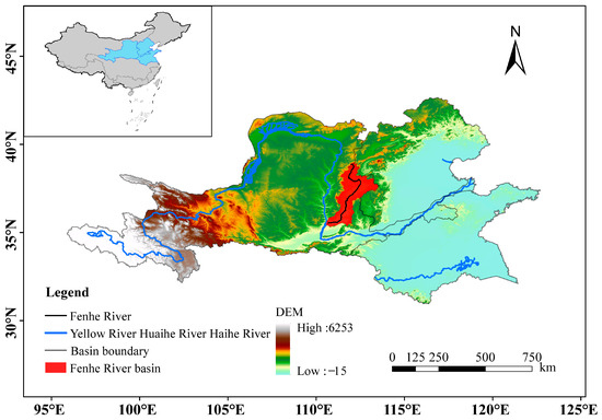
Figure 1.
The study area of the Fenhe River basin, which is located in the middle of the HHH basin. The blue and black lines represent the river, and the red part is the FHR basin.
2.2. Datasets
Interpolated meteorological data are used in this study, and the variables are shown in Table 1. These data were developed by interpolating observations from more than 2400 ground-based meteorological stations in China [47]. Our study used data from 1961 to 2020; all variables were based on daily data with a spatial resolution of 0.5° × 0.5°. Since atmospheric stress on evapotranspiration is an essential factor of land drought, we further calculated daily potential evapotranspiration (PET) and vapor pressure deficit (VPD) from interpolated daily observations, which were then used as inputs of the model [35,38,48].

Table 1.
Meteorological variables used in this study.
We used the data from 1961 to 2000 as a training set and those from 2001 to 2010 as a validation set. And we used data from 2011 to 2020 to evaluate the model’s performance. The ratio of the training set, validation set, and test set was 4:1:1. For network prediction, the data of the previous 30 days were used to forecast drought conditions in the FHR basin for the next 10 days, resulting in a total of 14,461 training samples, and both the validation set and the test set contained 3611 samples each. To accelerate the model convergence, we standardized the data pixel-wisely using Equation (1). X*t indicates the value after standardization at time t.
where Xt denotes the grid value for a day at a certain latitude and longitude, Xmin denotes the minimum value on the corresponding latitude and longitude time series, and Xmax denotes the maximum value on the corresponding latitude and longitude time series.
2.3. Methods
2.3.1. SAPEI Calculation
The daily SAPEI was used as a measure of drought in the FHR basin [38]. The calculation of the SAPEI requires the construction of the daily difference between precipitation (PRE) and PET, which can be estimated by Equation (2). The Penman–Monteith method was used to estimate PET, which has a more physical basis than other methods [49].
In Equation (2), D indicates the daily difference between PRE and PET, a is the attenuation constant, N is the number of days ahead, and c is the fraction of contribution of the last day of precipitation. Based on previous studies [38,50], a = 0.98 and c = 13%, resulting in N = 100. After that, we could obtain the SAPEI based on the sequence D [35,51].
The SAPEI values were divided into nine classes, namely extreme wet, severe wet, moderate wet, mild wet, normal, mild drought, moderate drought, severe drought, and extreme drought, as detailed in Table 2 [52]. We calculated the cumulative probability of the SAPEI in the test set in order to facilitate the evaluation of the forecast results at a later stage.
Table 2.
Different categories of SAPEI.
2.3.2. The A_CNN Model
The A_CNN model was used to predict the daily SAPEI [30]. This model combines the advantages of the CNN in spatial information processing, comprehensively considers the influence of the surrounding climate environment on the FHR basin, and learns the characteristics of continuous changes in drought in different seasons. It contains three convolutional layers. After convolutional layer1 and layer2, a max pooling layer is connected, and the three convolution layers are followed by two fully connected layers (as shown in Figure 2). We set a fixed time step p for the historical data X = {xt, xt−1, …, xt−p} as input time series, where xt is the value of the variable at time t. The model output was a time series Y with length q, Y = {xt+1, xt+2, …, xt+q}. For defining p and q, we needed to pay attention to the periodic characteristics of the original data, so we set the time step to one month (30 days), and the output time of the model was 10 days. In our study, the input data were the spatio-temporal cubes of two sets of variables at time t − 30 to t − 1, and the output was the average value of the SAPEI index of the FHR basin from t + 0 to t + 10 days. M denotes the number of convolutional kernels (the value is 10), and N denotes the number of nodes in the FC layer (the value is 50). It is worth noting that our inputs were multiple spatio-temporal datasets with a spatial range of (95°~123° E, 30°~43° N), which was different from the traditional multivariate time series forecasting. The SAPEI index of the FHR basin was spatially averaged to show the basin-scale drought, which was used as the output of the model.
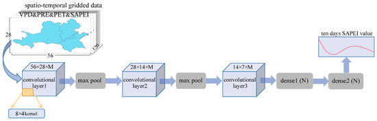
Figure 2.
The core structure of the model consists of three convolutional layers, two max-pooling layers, two fully connected layers, and an output layer. Model components are differentiated by color and the red wavy line indicates the SAPEI value.
In the training process, the convolutional kernel size was set to 8 × 4 in the first convolutional layer and to 4 × 2 in the last two convolutional layers. The number of epochs was 100, with each epoch containing 56 iterations, and the Adam optimizer was used. The hyperbolic tangent function (tanh) was used for the activation function, and the learning rate of training was fixed at 0.0005. The output shapes of each layer in the model are summarized in Table 3.
Table 3.
Output shape for each layer of the model.
PRE, PET, and VPD play a crucial role in the water cycle and have significant impacts on the variability in drought levels in a region [53,54,55]. VPD is mainly expressed as the difference between the water vapor pressure at saturation and the actual water vapor pressure at a certain temperature [48,56]. To improve the prediction accuracy and speed up the convergence of the model, we designed two sets of experiments for comparison. In the first experiment, the SAPEI and three important variables affecting drought (PRE, PET, VPD) were used as input variables, which we named EXP4. In the second experiment, we took all meteorological variables as input (as shown in Table 1), which we named EXP10. We wanted to explore whether we could improve the prediction accuracy by capturing the key factors affecting drought.
2.3.3. Evaluation Metrics
To evaluate the model performance, the mean squared error (MSE) was used as the loss function; the mean absolute error (MAE), BIAS, Nash–Sutcliffe efficiency (NSE), Kling–Gupta efficiency (KGE), and the Pearson correlation coefficient (R) were also calculated for the test set. To minimize the impact of RMSE deviations, we employed the unbiased root mean square difference (ubRMSD) metric, which combines R and standard deviation (Std) to evaluate the effect of EXP4 and EXP10. The calculation of the evaluation metrics is summarized as follows:
In Equations (4)–(9), yi denotes the value of SAPEI on day i, yi′ denotes the predicted value, α denotes the ratio between the Std of predicted results and the Std of true values, and β denotes the ratio between the mean of predicted results and the mean of true values. Var(y) and Var(y′) mean the variance in the observations and predictions, and Cov(y,y′) is their covariance.
3. Results
3.1. Identifying Key Variables to Enhance Prediction Accuracy
In this experiment, the SAPEI was predicted for the next 10 days in the FHR basin. Non-meteorological parameters such as the SAPEI were calculated in our study; we removed non-meteorological parameters and trained the model, which we named EXP7. Table 4 shows the prediction results for all parameters (EXP10) and the removal of non-meteorological parameters (EXP7). We show the predictions for days 1, 3, 5, 7, and 9, and the five prediction lengths are denoted as PL1, PL3, PL5, PL7, and PL9. When we remove the non-meteorological parameters, the model’s prediction results significantly deteriorate and become inaccurate. A higher R and lower MSE indicate a better prediction effect. The R value for the predicted results of EXP7, as shown in Table 4, is significantly lower than that of EXP10, while the MSE is noticeably higher than that of EXP10. Non-meteorological parameters play a crucial role in the prediction process. Therefore, we chose to include non-meteorological parameters in both sets of comparative experiments.
Table 4.
Comparison of results for different prediction lengths.
We compared the predictions on day 1, 3, 5, 7, and 9 from two experiments. A Taylor diagram is used to compare the evaluation metrics between predicted and actual values. Figure 3 displays the training results obtained using two experiments for different prediction lengths (indicated by colors). The R values range from 0.8 to 0.96, indicating that both experiments have achieved good results for different prediction lengths. However, upon comparison, it was concluded that the results obtained by training with EXP4 were significantly better than EXP10. This is evident in the distribution of the squares, which is consistently below the circles of the same color, indicating a higher correlation than the results obtained by training with all variables. In addition, the ubRMSD of EXP4 is significantly lower than EXP10, which shows that for different prediction lengths, EXP4 gives better results than EXP10. The Std in the Taylor diagram is the ratio value between the Std of predicted data from the model and true values. The ratio closer to 1 indicates the better prediction of results. As can be seen from the Taylor diagram, for a prediction length of 3, EXP10 is slightly better than EXP4. However, EXP4 outperforms EXP10 in the rest of the predicted lengths. Combining the three evaluation metrics, EXP4 achieves a better performance. To verify this conclusion, the test set samples of the two experiments were stitched together, and the MSE was calculated for predicting day one to day ten, respectively. The mean of the ten-day prediction MSE reached 0.169 for the EXP4 and only 0.272 for the mean of the EXP10, which further confirms the previous conclusion.
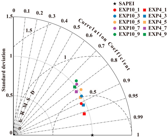
Figure 3.
Comparison of the results of EXP4 and EXP10: We record the predictions for the two sets of experiments one day ahead as EXP4_1 and EXP10_1, and so on. The Taylor diagram shows the predictive effect of different models in considering Standard deviation (dotted), Correlation Coefficient (alternating lines and dots), and ubRMSD (dashed).
While deep learning methods often require a substantial amount of data to produce optimal results, the size of the dataset does not always guarantee improved performance. The properties of the data and the model itself can significantly impact the training outcome, and it is essential to evaluate them within the context of the specific experiment. In our experiment, we obtained favorable outcomes for EXP4. By focusing on the important variables, the model could more easily discern the time series’ characteristics. Furthermore, increasing the data quantity did not improve the results, so we mainly present the EXP4 findings in the following section.
The MAE is commonly used to assess the deviation between the predicted and actual SAPEI values; it is calculated in a way that avoids the influence of some extreme values on the overall results, making the results more stable [57,58,59]. Figure 4 shows that the MAE of the test set gradually rises as the prediction length increases. The MAE for each prediction length is shown as a red line, and the shaded area indicates the standard deviation. Although the effect becomes progressively worse as the prediction length increases, the MAE for the next ten-day forecast of the FHR basin remains stable below 0.4, indicating that the model’s performance is generally relatively consistent.
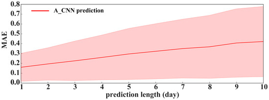
Figure 4.
The MAE from 1- to 10-day prediction, and the shaded area indicates the standard deviation.
This study also applied the NSE and KGE to evaluate the model’s predictions; Table 5 shows the different evaluation metrics of the model in the test set. It can be seen from Table 5 that the model’s predictions are more accurate when the prediction length is 1 day (PL1) or 3 days (PL3). However, the model’s predictions deteriorate when the prediction length increases. When the prediction length changes to 9 days (PL9), the R of the predicted results is acceptable, and in terms of the KGE, the model does not give accurate predictions.
Table 5.
Evaluation metrics for models with different prediction lengths.
In order to provide a more intuitive representation of the model’s prediction performance, we extracted the prediction results on days 1, 3, 5, 7, and 9 for the test set samples and plotted time series graphs for comparison. Figure 5 displays the time series of predicted values and true values from 2011 to 2020. The true value is represented by the black line, which is the SAPEI calculated from meteorological data. The other five colors correspond to the five different prediction lengths. For each predicted time series, we calculated the R and MSE. The model performed the best in predicting the next day, with an R of 0.96. As the prediction time increased, the effect of model deteriorated slightly, but the overall performance remained relatively stable. Severe drought events were defined as SAPEI values below −1.5, which are represented by a black dashed line in the figure. Although the frequency of severe drought events in the FHR basin was low over the past decade, the model accurately predicted them. Additionally, the model showed promising performance in predicting gradual climate changes from wet to drought conditions.
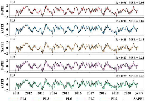
Figure 5.
The true and predicted SAPEI values; five different prediction lengths were selected for presentation. The black line indicates true SAPEI values, and the other colored lines indicate 1-day, 3-day, 5-day, 7-day, and 9-day predictions, respectively. The dotted line indicates a SAPEI value of −1.5, beyond which, it is a severe drought.
Then, the prediction performances of different SAPEI categories as listed in Table 2 were evaluated using the ten-year test dataset spanning from 2011 to 2020 (as shown in Figure 6). Clearly, the prediction bias increased for SAPEI extremes with increasing prediction lengths. From a model training perspective, this is not unexpected since the SAPEI has fewer extreme samples, making it difficult for the model to learn their features, leading to relatively poor prediction skills. It is striking to find that the used model overestimated the drought conditions and underestimated the wet conditions. The prediction biases of drought events are relatively smaller than those of wet events, indicating the better performance of the used model for drought prediction.
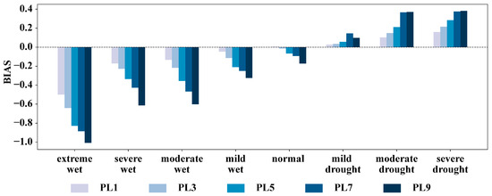
Figure 6.
The prediction BIAS of each SAPEI category at different prediction lengths.
3.2. Predicting Severe Drought
We used a case of severe drought to evaluate the model performance. In early 2019, there was high temperature with significant precipitation deficit in the HHH region, leading to a severe drought. Such a drought event is reflected in the SAPEI data, and thus, we used it for the case study. In Figure 7a, 1-day, 3-day, 5-day, 7-day, and 9-day predictions against the realistic SAPEI values are shown. There was significant precipitation deficit in March, and PET was increasing due to high temperature, which caused a decreasing SAPEI and thus a severe drought. In April, several precipitation events alleviated the drought. It appears that the basin-scale severe drought event was well predicted by the used model, especially when short prediction lengths were used, suggesting the model’s credibility in the prediction of extreme events.
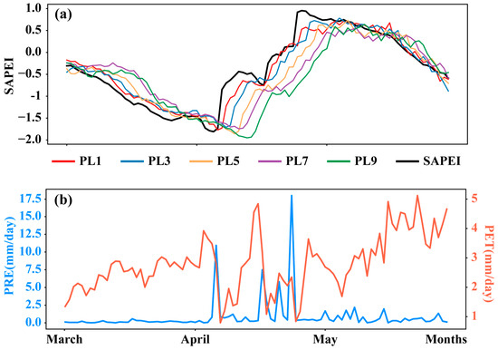
Figure 7.
(a) The SAPEI predictions in early 2019 in the FHR basin. The black line represents the real SAPEI value, and the other colored lines represent the predictions at different lengths. (b) The PRE and PET.
4. Discussion
In this study, the SAEPI was selected as a drought index to assess drought conditions in the FHR basin. We used a deep learning approach to predict the next 10 days of drought in the FHR basin. Overall, the predictions of the model are accurate. As shown in Figure 5, the model’s R reaches 0.79 even when the prediction length is 9 days. However, the accuracy of model predictions inevitably decreases as the length of the prediction increases; this is also consistent with previous research [60]. The higher prediction accuracy obtained by using fewer key variables for training also reflects that deep learning can overcome the limitations of numerical weather prediction [61,62]. Xu et al. [26] have demonstrated that deep learning methods can efficiently process time series, while our study takes spatial factors into account, making the prediction of drought more scientific. The training data for the model contain non-meteorological parameters, which also has some limitations. Non-meteorological parameters enhance prediction accuracy, but they are calculated from meteorological parameters and are not independent.
Although the experiment used these as key variables affecting drought, it does not mean that the other variables have little influence on drought. Temperature changes can also have a significant impact on drought conditions [63]. We also tried to add variables such as temperature and wind speed for training; the results were stable, but the optimal solution was not obtained. We need to note that a single increase in predictors does not necessarily improve model performance [19]. Dikshit et al. [64] mentioned that exploring the effects of different meteorological elements in drought prediction can improve the accuracy of predictions. The purpose of this study is to make timely and effective predictions of short-term drought; this contributes to a timely response by policy makers, farmers, and other stakeholders [65].
In our study, we calculated mean values for the SAPEI within the FHR basin to produce labels for our model. While this approach provides an overview of the drought situation in the study area, it also presents a challenge of weakening extreme values that could significantly impact the overall analysis. In addition, predictor selection plays an important role in drought prediction [25]. Our study takes into account the influence of the spatial environment; in addition to natural factors, the impact of human activities on climate change should not be ignored. Combining the impact of multiple factors will allow us to refine our model, contributing to the development of better disaster prevention strategies.
5. Conclusions
Our study utilized a deep learning method to predict drought in the FHR basin on a daily scale. Our methodology takes into account the effects of multiple meteorological elements and spatial scales on drought. The results of the study show that the prediction accuracy of the model decreases with increasing prediction lengths. As can be seen in Table 4, the NSE of the prediction results reaches 0.922 when the prediction length is 1 day, but the accuracy of the model decreases when the prediction length increases. The long-term prediction of the model did not reach a high level of confidence in terms of the KGE. However, previous studies have also demonstrated that this is an acceptable phenomenon.
It is concluded from our study that for predicting drought in the FHR basin, EXP4, which used the important variables affecting drought as network inputs, obtained a better result compared to EXP10. We used relatively little data to obtain better predictions. Capturing the characteristics of several important variables that affect drought allows the model to make more effective predictions. This reduces computational costs significantly compared to traditional numerical weather prediction methods [62].
The model is able to capture fluctuations in SAPEI and predict heavy drought events in advance, which effectively mitigates the losses caused by natural disasters. Timely access to drought-related early warning information is key for early warning institutions to select adaptation strategies [66]. Therefore, this research has important implications in drought prevention.
Author Contributions
Conceptualization, Z.C., G.W. and X.W.; methodology, Z.C. and X.W.; software, Z.C.; validation, Z.C. and G.W.; formal analysis, Z.C. and Y.H.; resources, H.J.; data curation, Z.C.; writing—original draft preparation, Z.C.; writing—review and editing, G.W. and Z.D.; visualization, Z.C.; supervision, G.W., X.W. and Y.L.; project administration, G.W.; funding acquisition, G.W. All authors have read and agreed to the published version of the manuscript.
Funding
This research was funded by the National Natural Science Foundation of China, grant number 42275028.
Institutional Review Board Statement
Not applicable.
Informed Consent Statement
Not applicable.
Data Availability Statement
Data are contained within the article.
Acknowledgments
We thank the researchers or teams who provided the basic data. We also thank the authors, reviewers, and editors who made amendments to the article.
Conflicts of Interest
The authors declare no conflicts of interest.
References
- Dikshit, A.; Pradhan, B.; Huete, A.; Park, H.-J. Spatial based drought assessment: Where are we heading? A review on the current status and future. Sci. Total Environ. 2022, 844, 157239. [Google Scholar] [CrossRef] [PubMed]
- Shi, H.; Zhou, Z.; Liu, L.; Liu, S. A global perspective on propagation from meteorological drought to hydrological drought during 1902–2014. Atmos. Res. 2022, 280, 106441. [Google Scholar] [CrossRef]
- Jehanzaib, M.; Yoo, J.; Kwon, H.-H.; Kim, T.-W. Reassessing the frequency and severity of meteorological drought considering non-stationarity and copula-based bivariate probability. J. Hydrol. 2021, 603, 126948. [Google Scholar] [CrossRef]
- Gavahi, K.; Abbaszadeh, P.; Moradkhani, H. How does precipitation data influence the land surface data assimilation for drought monitoring? Sci. Total Environ. 2022, 831, 154916. [Google Scholar] [CrossRef] [PubMed]
- Wang, C.; Chen, J.; Gu, L.; Wu, G.; Tong, S.; Xiong, L.; Xu, C.-Y. A pathway analysis method for quantifying the contributions of precipitation and potential evapotranspiration anomalies to soil moisture drought. J. Hydrol. 2023, 621, 129570. [Google Scholar] [CrossRef]
- Han, L.; Zhang, Q.; Zhang, Z.; Jia, J.; Wang, Y.; Huang, T.; Cheng, Y. Drought area, intensity and frequency changes in China under climate warming, 1961–2014. J. Arid Environ. 2021, 193, 104596. [Google Scholar] [CrossRef]
- Xu, Y.; Zhu, X.; Cheng, X.; Gun, Z.; Lin, J.; Zhao, J.; Yao, L.; Zhou, C. Drought assessment of China in 2002–2017 based on a comprehensive drought index. Agric. For. Meteorol. 2022, 319, 108922. [Google Scholar] [CrossRef]
- Su, B.; Huang, J.; Fischer, T.; Wang, Y.; Kundzewicz, Z.W.; Zhai, J.; Sun, H.; Wang, A.; Zeng, X.; Wang, G. Drought losses in China might double between the 1.5 C and 2.0 C warming. Proc. Natl. Acad. Sci. USA 2018, 115, 10600–10605. [Google Scholar] [CrossRef]
- Wang, Z.; Li, J.; Lai, C.; Zeng, Z.; Zhong, R.; Chen, X.; Zhou, X.; Wang, M. Does drought in China show a significant decreasing trend from 1961 to 2009? Sci. Total Environ. 2017, 579, 314–324. [Google Scholar] [CrossRef]
- Shi, X.; Ding, H.; Wu, M.; Zhang, N.; Shi, M.; Chen, F.; Li, Y. Effects of different types of drought on vegetation in Huang-Huai-Hai River Basin, China. Ecol. Indic. 2022, 144, 109428. [Google Scholar] [CrossRef]
- Zhan, C.; Liang, C.; Zhao, L.; Jiang, S.; Niu, K.; Zhang, Y. Drought-related cumulative and time-lag effects on vegetation dynamics across the Yellow River Basin, China. Ecol. Indic. 2022, 143, 109409. [Google Scholar] [CrossRef]
- Zhang, X.; Duan, Y.; Duan, J.; Chen, L.; Jian, D.; Lv, M.; Yang, Q.; Ma, Z. A daily drought index-based regional drought forecasting using the Global Forecast System model outputs over China. Atmos. Res. 2022, 273, 106166. [Google Scholar] [CrossRef]
- Balti, H.; Abbes, A.B.; Mellouli, N.; Farah, I.R.; Sang, Y.; Lamolle, M. A review of drought monitoring with big data: Issues, methods, challenges and research directions. Ecol. Inf. 2020, 60, 101136. [Google Scholar] [CrossRef]
- Durdu, Ö.F. Application of linear stochastic models for drought forecasting in the Büyük Menderes river basin, western Turkey. Stoch. Environ. Res. Risk Assess. 2010, 24, 1145–1162. [Google Scholar] [CrossRef]
- Li, H.; Sun, B.; Wang, H.; Zhou, B.; Duan, M. Mechanisms and physical-empirical prediction model of concurrent heatwaves and droughts in July–August over northeastern China. J. Hydrol. 2022, 614, 128535. [Google Scholar] [CrossRef]
- Prodhan, F.A.; Zhang, J.; Hasan, S.S.; Sharma, T.P.P.; Mohana, H.P. A review of machine learning methods for drought hazard monitoring and forecasting: Current research trends, challenges, and future research directions. Environ. Model. Softw. 2022, 149, 105327. [Google Scholar] [CrossRef]
- Feng, P.; Wang, B.; Li Liu, D.; Yu, Q. Machine learning-based integration of remotely-sensed drought factors can improve the estimation of agricultural drought in South-Eastern Australia. Agric. Syst. 2019, 173, 303–316. [Google Scholar] [CrossRef]
- Nie, H.; Yang, L.; Li, X.; Ren, L.; Xu, J.; Feng, Y. Spatial prediction of soil moisture content in winter wheat based on machine learning model. In Proceedings of the 2018 26th International Conference on Geoinformatics, Kunming, China, 28–30 June 2018; pp. 1–6. [Google Scholar]
- Dikshit, A.; Pradhan, B.; Santosh, M. Artificial neural networks in drought prediction in the 21st century–A scientometric analysis. Appl. Soft Comput. 2022, 114, 108080. [Google Scholar] [CrossRef]
- Nourani, V.; Baghanam, A.H.; Adamowski, J.; Kisi, O. Applications of hybrid wavelet–artificial intelligence models in hydrology: A review. J. Hydrol. 2014, 514, 358–377. [Google Scholar] [CrossRef]
- Coşkun, Ö.; Citakoglu, H. Prediction of the standardized precipitation index based on the long short-term memory and empirical mode decomposition-extreme learning machine models: The Case of Sakarya, Türkiye. Phys. Chem. Earth Parts A/B/C 2023, 131, 103418. [Google Scholar] [CrossRef]
- Zhang, X.; Jin, Q.; Yu, T.; Xiang, S.; Kuang, Q.; Prinet, V.; Pan, C. Multi-modal spatio-temporal meteorological forecasting with deep neural network. ISPRS J. Photogramm. Remote Sens. 2022, 188, 380–393. [Google Scholar] [CrossRef]
- Agana, N.A.; Homaifar, A. A deep learning based approach for long-term drought prediction. In Proceedings of the SoutheastCon 2017, Concord (Charlotte), NC, USA, 30 March–2 April 2017; pp. 1–8. [Google Scholar]
- Mokhtar, A.; Jalali, M.; He, H.; Al-Ansari, N.; Elbeltagi, A.; Alsafadi, K.; Abdo, H.G.; Sammen, S.S.; Gyasi-Agyei, Y.; Rodrigo-Comino, J. Estimation of SPEI meteorological drought using machine learning algorithms. IEEE Access 2021, 9, 65503–65523. [Google Scholar] [CrossRef]
- Mei, P.; Liu, J.; Liu, C.; Liu, J. A deep learning model and its application to predict the monthly MCI drought index in the Yunnan Province of China. Atmosphere 2022, 13, 1951. [Google Scholar] [CrossRef]
- Xu, Z.; Sun, H.; Zhang, T.; Xu, H.; Wu, D.; Gao, J. Evaluating established deep learning methods in constructing integrated remote sensing drought index: A case study in China. Agric. Water Manag. 2023, 286, 108405. [Google Scholar] [CrossRef]
- Dirmeyer, P.A.; Brubaker, K.L. Characterization of the global hydrologic cycle from a back-trajectory analysis of atmospheric water vapor. J. Hydrometeorol. 2007, 8, 20–37. [Google Scholar] [CrossRef]
- Wei, J.; Dirmeyer, P.A. Sensitivity of land precipitation to surface evapotranspiration: A nonlocal perspective based on water vapor transport. Geophys. Res. Lett. 2019, 46, 12588–12597. [Google Scholar] [CrossRef]
- Ham, Y.-G.; Kim, J.-H.; Luo, J.-J. Deep learning for multi-year ENSO forecasts. Nature 2019, 573, 568–572. [Google Scholar] [CrossRef]
- Ham, Y.-G.; Kim, J.-H.; Kim, E.-S.; On, K.-W. Unified deep learning model for El Niño/Southern Oscillation forecasts by incorporating seasonality in climate data. Sci. Bull. 2021, 66, 1358–1366. [Google Scholar] [CrossRef]
- Hao, Z.; Singh, V.P. Drought characterization from a multivariate perspective: A review. J. Hydrol. 2015, 527, 668–678. [Google Scholar] [CrossRef]
- Palmer, W.C. Meteorological Drought; US Department of Commerce, Weather Bureau: Washington, DC, USA, 1965; Volume 30.
- Wells, N.; Goddard, S.; Hayes, M.J. A self-calibrating Palmer drought severity index. J. Clim. 2004, 17, 2335–2351. [Google Scholar] [CrossRef]
- McKee, T.B.; Doesken, N.J.; Kleist, J. The relationship of drought frequency and duration to time scales. In Proceedings of the 8th Conference on Applied Climatology, Anaheim, CA, USA, 17–22 January 1993; pp. 179–183. [Google Scholar]
- Vicente-Serrano, S.M.; Beguería, S.; López-Moreno, J.I. A multiscalar drought index sensitive to global warming: The standardized precipitation evapotranspiration index. J. Clim. 2010, 23, 1696–1718. [Google Scholar] [CrossRef]
- Wang, L.; Chen, W. Applicability analysis of standardized precipitation evapotranspiration index in drought monitoring in China. Plateau Meteorol. 2014, 33, 423–431. [Google Scholar]
- Yuan, X.; Wang, Y.; Ji, P.; Wu, P.; Sheffield, J.; Otkin, J.A. A global transition to flash droughts under climate change. Science 2023, 380, 187–191. [Google Scholar] [CrossRef]
- Li, J.; Wang, Z.; Wu, X.; Xu, C.-Y.; Guo, S.; Chen, X. Toward monitoring short-term droughts using a novel daily scale, standardized antecedent precipitation evapotranspiration index. J. Hydrometeorol. 2020, 21, 891–908. [Google Scholar] [CrossRef]
- Hao, Z.; Singh, V.P.; Xia, Y. Seasonal drought prediction: Advances, challenges, and future prospects. Rev. Geophys. 2018, 56, 108–141. [Google Scholar] [CrossRef]
- Park, S.; Seo, E.; Kang, D.; Im, J.; Lee, M.-I. Prediction of drought on pentad scale using remote sensing data and MJO index through random forest over East Asia. Remote Sens. 2018, 10, 1811. [Google Scholar] [CrossRef]
- Wu, B.; Yang, S.; Shao, N.; Peng, R.; Guan, Y. Effects of land use change on ecosystem service value in fragile ecological area of the Loess Plateau a case study of Fenhe River Basin. Soil Water Conserv. 2019, 26, 340–345. [Google Scholar]
- Yan, D.; Wu, D.; Huang, R.; Wang, L.; Yang, G. Drought evolution characteristics and precipitation intensity changes during alternating dry–wet changes in the Huang–Huai–Hai River basin. Hydrol. Earth Syst. Sci. 2013, 17, 2859–2871. [Google Scholar] [CrossRef]
- Yuan, Y.; Yan, D.; Yuan, Z.; Yin, J.; Zhao, Z. Spatial distribution of precipitation in huang-huai-Hai River basin between 1961 to 2016, China. Int. J. Environ. Res. Public Health 2019, 16, 3404. [Google Scholar] [CrossRef]
- Hu, W.; She, D.; Xia, J.; He, B.; Hu, C. Dominant patterns of dryness/wetness variability in the Huang-Huai-Hai River Basin and its relationship with multiscale climate oscillations. Atmos. Res. 2021, 247, 105148. [Google Scholar] [CrossRef]
- Deng, Y.; Wu, D.; Wang, X.; Xie, Z. Responding time scales of vegetation production to extreme droughts over China. Ecol. Indic. 2022, 136, 108630. [Google Scholar] [CrossRef]
- Li, C.; Kattel, G.R.; Zhang, J.; Shang, Y.; Gnyawali, K.R.; Zhang, F.; Miao, L. Slightly enhanced drought in the Yellow River Basin under future warming scenarios. Atmos. Res. 2022, 280, 106423. [Google Scholar] [CrossRef]
- Wu, J.; Gao, X.-J. A gridded daily observation dataset over China region and comparison with the other datasets. Chin. J. Geophys. 2013, 56, 1102–1111. [Google Scholar]
- Yuan, W.; Zheng, Y.; Piao, S.; Ciais, P.; Lombardozzi, D.; Wang, Y.; Ryu, Y.; Chen, G.; Dong, W.; Hu, Z. Increased atmospheric vapor pressure deficit reduces global vegetation growth. Sci. Adv. 2019, 5, eaax1396. [Google Scholar] [CrossRef]
- Allen, R.G.; Pereira, L.S.; Raes, D.; Smith, M. Crop evapotranspiration-Guidelines for computing crop water requirements-FAO Irrigation and drainage paper 56. Fao Rome 1998, 300, D05109. [Google Scholar]
- Heggen, R.J. Normalized antecedent precipitation index. J. Hydrol. Eng. 2001, 6, 377–381. [Google Scholar] [CrossRef]
- Chen, J.; Yu, W.; Liu, R.; Yue, W.; Chen, X. Daily standardized antecedent precipitation evapotranspiration index (SAPEI) and its adaptability in Anhui Province. Chin. J. Eco-Agric. 2019, 27, 919–928. [Google Scholar]
- Miah, M.G.; Abdullah, H.M.; Jeong, C. Exploring standardized precipitation evapotranspiration index for drought assessment in Bangladesh. Environ. Monit. Assess. 2017, 189, 547. [Google Scholar] [CrossRef]
- Ma, T.; Liang, Y.; Lau, M.K.; Liu, B.; Wu, M.M.; He, H.S. Quantifying the relative importance of potential evapotranspiration and timescale selection in assessing extreme drought frequency in conterminous China. Atmos. Res. 2021, 263, 105797. [Google Scholar] [CrossRef]
- Cook, B.I.; Smerdon, J.E.; Seager, R.; Coats, S. Global warming and 21st century drying. Clim. Dyn. 2014, 43, 2607–2627. [Google Scholar] [CrossRef]
- Oogathoo, S.; Houle, D.; Duchesne, L.; Kneeshaw, D. Vapour pressure deficit and solar radiation are the major drivers of transpiration of balsam fir and black spruce tree species in humid boreal regions, even during a short-term drought. Agric. For. Meteorol. 2020, 291, 108063. [Google Scholar] [CrossRef]
- Li, M.; Yao, J.; Guan, J.; Zheng, J. Observed changes in vapor pressure deficit suggest a systematic drying of the atmosphere in Xinjiang of China. Atmos. Res. 2021, 248, 105199. [Google Scholar] [CrossRef]
- Legates, D.R.; McCabe, G.J., Jr. Evaluating the use of “goodness-of-fit” measures in hydrologic and hydroclimatic model validation. Water Resour. Res. 1999, 35, 233–241. [Google Scholar] [CrossRef]
- Jayasinghe, W.L.P.; Deo, R.C.; Ghahramani, A.; Ghimire, S.; Raj, N. Development and evaluation of hybrid deep learning long short-term memory network model for pan evaporation estimation trained with satellite and ground-based data. J. Hydrol. 2022, 607, 127534. [Google Scholar] [CrossRef]
- Ayris, D.; Imtiaz, M.; Horbury, K.; Williams, B.; Blackney, M.; See, C.S.H.; Shah, S.A.A. Novel deep learning approach to model and predict the spread of COVID-19. Intell. Syst. Appl. 2022, 14, 200068. [Google Scholar] [CrossRef]
- Dai, R.; Wang, W.; Zhang, R.; Yu, L. Multimodal deep learning water level forecasting model for multiscale drought alert in Feiyun River basin. Expert Syst. Appl. 2023, 244, 122951. [Google Scholar] [CrossRef]
- Abdulla, N.; Demirci, M.; Ozdemir, S. Design and evaluation of adaptive deep learning models for weather forecasting. Eng. Appl. Artif. Intell. 2022, 116, 105440. [Google Scholar] [CrossRef]
- Ren, X.; Li, X.; Ren, K.; Song, J.; Xu, Z.; Deng, K.; Wang, X. Deep learning-based weather prediction: A survey. Big Data Res. 2021, 23, 100178. [Google Scholar] [CrossRef]
- Hu, J.; Yang, Z.; Hou, C.; Ouyang, W. Compound risk dynamics of drought by extreme precipitation and temperature events in a semi-arid watershed. Atmos. Res. 2023, 281, 106474. [Google Scholar] [CrossRef]
- Dikshit, A.; Pradhan, B. Interpretable and explainable AI (XAI) model for spatial drought prediction. Sci. Total Environ. 2021, 801, 149797. [Google Scholar] [CrossRef]
- Otkin, J.A.; Woloszyn, M.; Wang, H.; Svoboda, M.; Skumanich, M.; Pulwarty, R.; Lisonbee, J.; Hoell, A.; Hobbins, M.; Haigh, T. Getting ahead of flash drought: From early warning to early action. Bull. Am. Meteorol. Soc. 2022, 103, E2188–E2202. [Google Scholar] [CrossRef]
- Ndiritu, S.W. Drought responses and adaptation strategies to climate change by pastoralists in the semi-arid area, Laikipia County, Kenya. Mitig. Adapt. Strategies Glob. Chang. 2021, 26, 10. [Google Scholar] [CrossRef]


Disclaimer/Publisher’s Note: The statements, opinions and data contained in all publications are solely those of the individual author(s) and contributor(s) and not of MDPI and/or the editor(s). MDPI and/or the editor(s) disclaim responsibility for any injury to people or property resulting from any ideas, methods, instructions or products referred to in the content. |
© 2024 by the authors. Licensee MDPI, Basel, Switzerland. This article is an open access article distributed under the terms and conditions of the Creative Commons Attribution (CC BY) license (https://creativecommons.org/licenses/by/4.0/).