Article

The Return Period Wind Speed Prediction of Beijing Urban Area Based on Short-Term Measured Wind Speed

Beijing’s Key Laboratory of Structural Wind Engineering and Urban Wind Environment, School of Civil Engineering, Beijing Jiaotong University, Beijing 100044, China
*
Author to whom correspondence should be addressed.
Atmosphere 2024, 15(2), 159; https://doi.org/10.3390/atmos15020159
Submission received: 24 December 2023 / Revised: 5 January 2024 / Accepted: 15 January 2024 / Published: 25 January 2024
(This article belongs to the Section Meteorology)

Abstract

:
To predict and explore the return period wind speed distribution in Beijing urban area, based on the short-term measured wind speed record, the measured independent storm peak samples are extracted and the Monte–Carlo numerical simulation method is used to randomly generate pseudo-independent storm peak samples with the same distribution as the independent storm peak samples. In addition, the appropriate threshold is used to select and extract the over-threshold independent storm peak samples from the measured samples. And, then, the return period wind speed of the whole wind direction is predicted. Further, the traditional Cook method is used to predict and analyze the return period wind speed of each wind direction according to the measured wind speed data. The results show that the return period wind speed prediction results of the whole wind direction corresponding to the simulated pseudo samples and the measured over-threshold samples are basically close to each other, and the maximum relative deviation is less than 7%. The mean relative deviation of the return period wind speed prediction results is about 10.6% between each wind direction and the whole wind direction, and the mean relative deviation is about 9.4% between the RPWS prediction result of each wind direction and the design value of the code. In addition, the return period wind speed prediction values of the west by southwest, northwest and north by northeast wind directions exceed the design value of the code, while the predicted values of the other wind directions are within the envelope range of the design value of the code. Finally, the research content of this paper can provide some reference for the wind resistance design analysis of building structures in Beijing area.

1. Introduction

On the west side of Jiande Bridge in Beijing, a 325 m high meteorological observation tower is equipped with wind speed measurement devices, obtaining the measured wind speed data with 10 min average intervals. Based on the measured data, it is essential to analyze the wind resistance of structures in the area to reasonably predict the return period wind speed (RPWS) for the Beijing urban area.
Based on the measured wind speed data, there is often a deficiency in the number of wind speed samples for RPWS prediction. And, when the annual maximum wind speed samples are selected to predict the RPWS, it is advisable to have no less than 10 years of measured wind speed data, with 25 years or more of data generally required to ensure prediction accuracy of the RPWS [1,2]. Therefore, when the observation period of the measured wind speed data is relatively short, making the most of existing measured wind speed information for RPWS prediction is a critical issue. Typically, the independent storm peak samples (ISPS) can be selected from the measured wind speed samples by using the independent storm method [3,4,5,6,7,8] and, to avoid the influence of small wind speed data on the prediction results, the over-threshold ISPS (OISPS) can be further screened and extracted by using the appropriate threshold. On the basis of the OISPS, the RPWS prediction analysis can be carried out by fitting the Generalized Pareto Distribution Model (GPDM) [9,10,11,12]. It is worth noting that, when using ISPS for extreme value distribution analysis, the process should ultimately be converted to annual extreme wind speed distribution analysis, but the issue of insufficient sample number still remains. Therefore, it is also possible to consider using the Monte–Carlo simulation method to generate pseudo-wind speed samples to increase the wind speed sample [13,14,15].
When generating pseudo-wind speed samples according to the Monte–Carlo simulation method, it is firstly necessary to determine the distribution type that the measured wind speed samples follow. Generally, the simulation analysis is conducted based on the distribution type of the measured daily maximum wind speed samples [15,16]. But it is prone to generating a significant number of low wind speed data, resulting in an overall underestimation of the pseudo-wind speed data, which can affect the results of RPWS prediction. Additionally, the pseudo-wind speed samples generated by Monte–Carlo simulation are assumed to be independent, while there is some level of correlation between the measured daily maximum wind speed samples. Thus, it cannot be guaranteed that the simulated samples will be relatively consistent with the measured wind speed samples. To ensure relative consistency between simulated samples and measured wind speed samples, an abundant amount of Pseudo-ISPS (PISPS) can be simulated based on the distribution of the measured ISPS using the Monte–Carlo method. This approach allows for making the best use of high wind speed information in the measured wind speed data while trying to keep the simulated samples as close to the measured ones as possible.
The analysis content of this paper is mainly divided into the following parts: in the first part, the statistical analysis of the short-term measured wind speed data is carried out. In the second part, the measured ISPS are extracted and a sufficient number of PISPS are generated by the Monte–Carlo simulation method. In the third part, PISPS was used to predict RPWS of the whole wind direction by using Extreme Value Type I (EVT I) distribution and Extreme Value Type III (EVT III) distribution models [17,18,19]. At the same time, the measured ISPS are filtered by a threshold to extract OISPS, and the GPDM is further used for RPWS prediction of the whole wind direction. In the fourth part, based on the measured 10 min average wind speed data, the wind speed samples in each wind direction are statistically extracted. Thus, the traditional Cook method is used to predict the RPWS value for each wind direction and a comparative analysis is conducted with the predicted results of the whole wind direction and the standard design value.

2. Measured Wind Speed Data Statistics

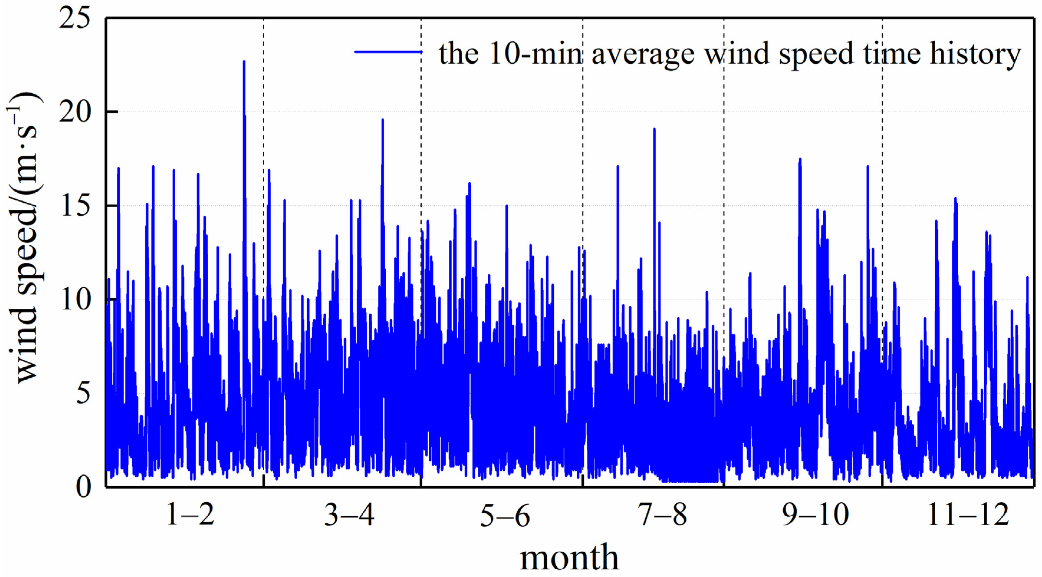
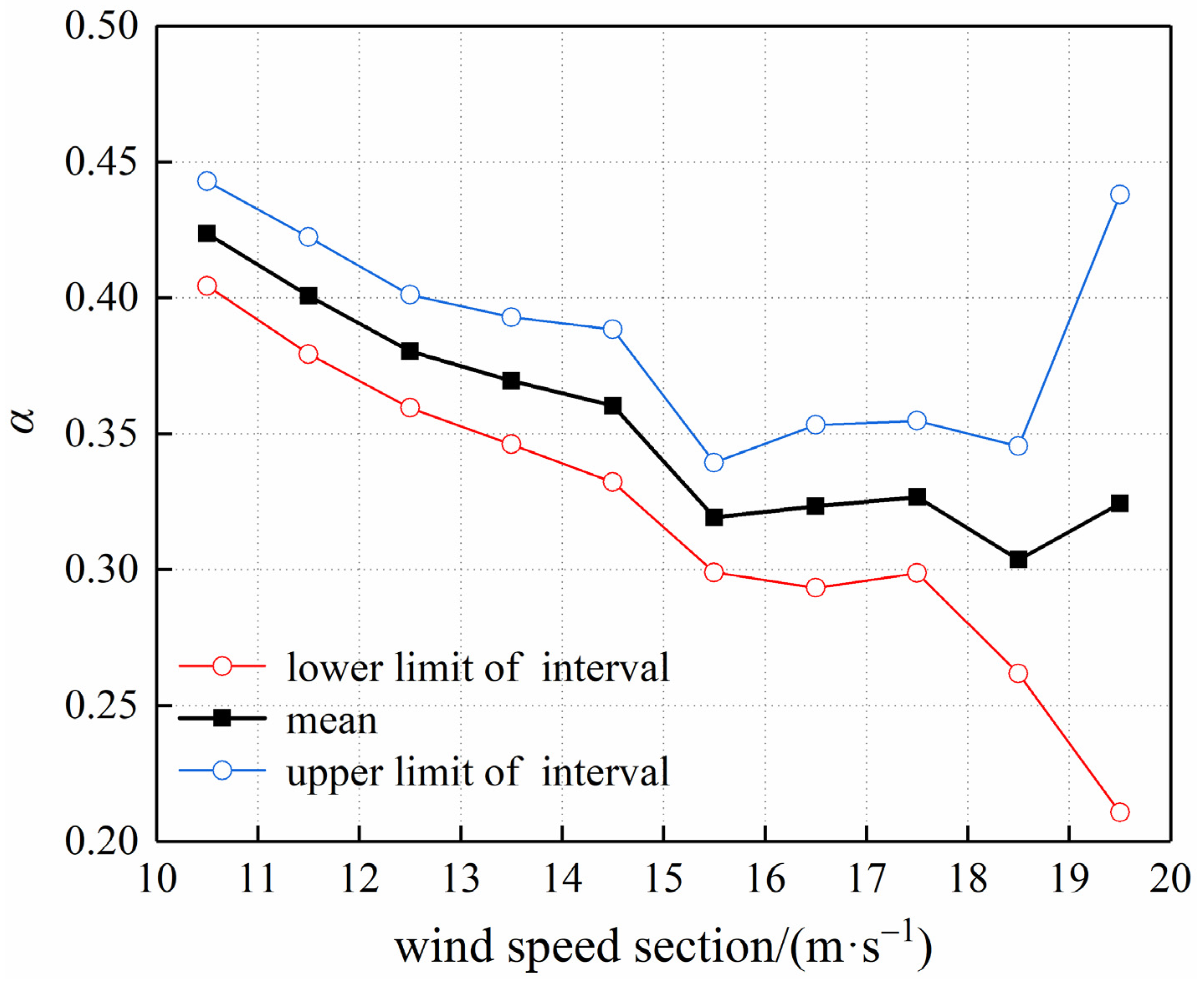
The meteorological tower is located in the northern part of Beijing city, west of the Jiande Bridge, as shown in Figure 1. The area around the meteorological tower features complex terrain, including park, roads, trees, and high-rise residential buildings with heights ranging from 60 to 90 m. The measured wind speed data from 2013 to 2017 at 15 different heights (8, 15, 32, 47, 65, 80, 100, 120, 140, 160, 180, 200, 240, 280 and 320 m) are selected for statistical analysis. And, according to Li et al. (2021), the wind speed spectrum characteristics of the measured wind speed data for the five years are representative [20], so the measured wind speed data from 2013 to 2017 can be used as the analysis sample. The measured wind speed sample time history is shown in Figure 2, taking the example of the 10 min average wind speed sample time history at a height of 200 m in 2015. And it is assumed that the average wind speed profile of Beijing city follows an exponential distribution, so the average wind profile index 𝛼 can be determined by fitting the measured wind speed data. In this process, firstly, the wind speed is divided into 10 wind speed sections from 10 to 20 m/s every interval of 1 m/s. The measured wind speed data of 5 years at the height of 200 m are taken as the analysis object, and the measured wind speed samples contained in each wind speed section are statistically extracted. According to the extracted measured wind speed samples of each wind speed section at 200 m height, the corresponding measured wind speed samples at the same date are extracted from each wind speed section at other heights. And, then, the average wind speed profile is fitted and determined, so as to obtain the corresponding average wind speed profile index 𝛼 samples in each wind speed section. Further, the mean and standard deviation values for 𝛼 samples are calculated in each wind speed section. Figure 3 shows the mean values and the upper and lower limits of the 95% confidence interval of the average wind speed profile index 𝛼 in different wind speed sections. As shown in Figure 3, the 𝛼 mean values in different wind speed sections tend to stabilize at 0.32 when the wind speed is greater than 15 m/s. However, the width of the 95% confidence interval of 𝛼 increases with the increase in wind speed values, which is mainly due to the increase in the data’s variability with the decrease in the wind speed sample number in the wind speed sections. Thus, a more stable 95% confidence interval of 𝛼 is selected as [0.29, 0.35]. The interval includes the 𝛼 value of 0.3 corresponding to the D type of geomorphology in the code. Therefore, this paper may wish to analyze the RPWS of Beijing city according to the type-D geomorphology. Considering the influence of factors such as urban development and construction on the roughness of the geomorphology within the urban area, the 𝛼 value of 0.32 is chosen as the average wind speed profile index. To reduce the influence of terrain factors around the meteorological tower on measured wind speed samples, the RPWS prediction is conducted using the measured daily maximum wind speed samples at a height of more than 100 m. In Figure 4, it represents an example using the measured daily maximum wind speed samples at a height of 200 m for the years 2013–2017.
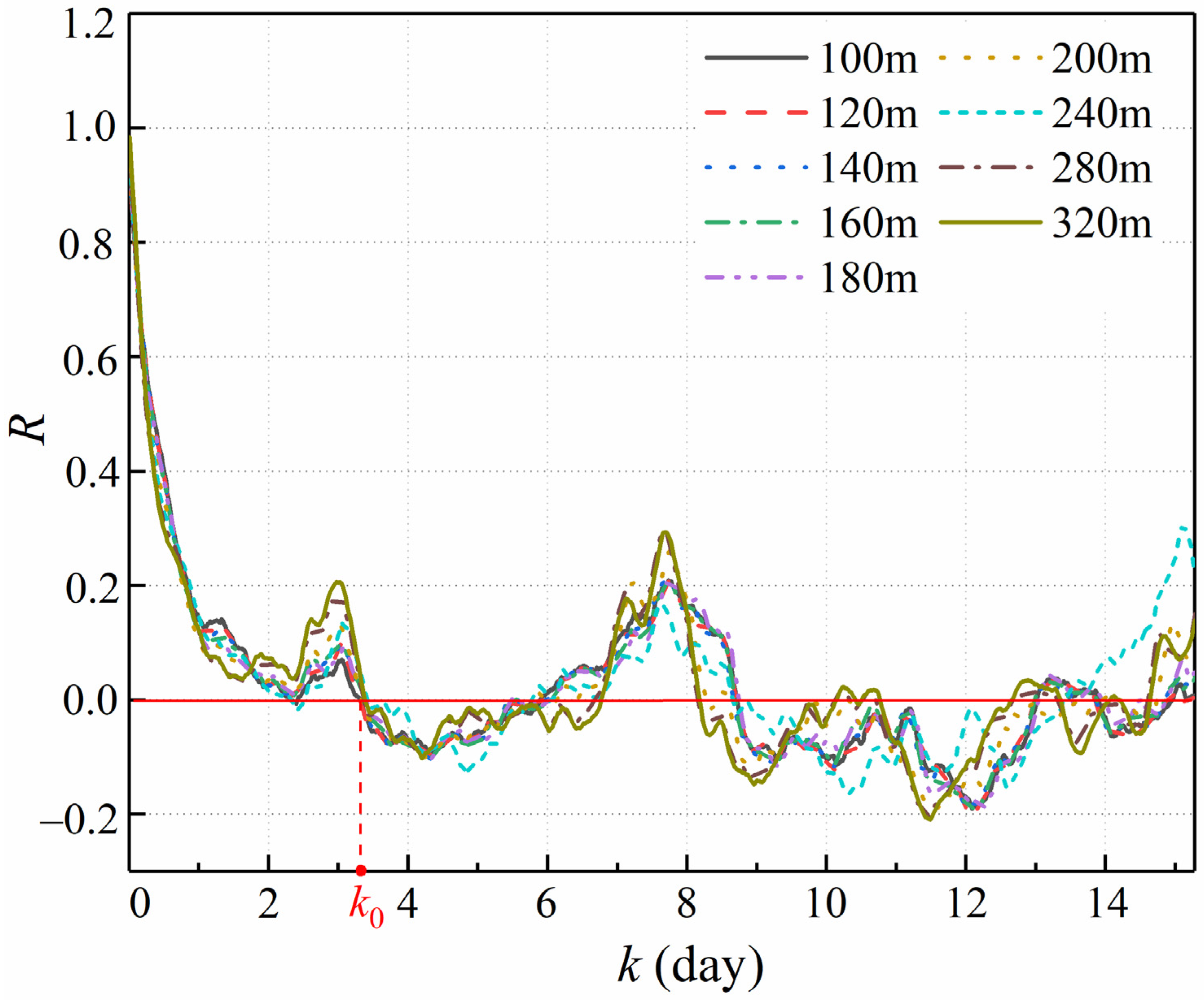
For the independence of the measured daily maximum wind speed samples, the duration of a single storm event is approximately 3–4 days according to the Van der Hoven wind speed spectrum theory. However, for the short-term measured wind speed samples, it may produce errors if the independence of samples is directly determined by the storm duration of 3–4 days [21], and the correlation characteristics of wind speed data themself are ignored. And the correlation between wind speed samples at different times in a wind speed sequence can be reflected by the autocorrelation coefficient. When the autocorrelation coefficient is not zero, the wind speeds are correlated. But, when the autocorrelation coefficient is zero, they are considered completely uncorrelated, that is, independent. Based on the time series of measured wind speed samples at heights of 100–320 m, the autocorrelation coefficients R corresponding to different time intervals k are calculated according to Equation (1). Thus, the relationship between R values of wind speed samples and k at different heights is obtained, as shown in Figure 5.
R k = E [ v l v ¯ · v l + k v ¯ ] σ v 2
where E · represents the expected value, v l and v l + k represent the wind speed sample values at times l and l + k, respectively. v ¯ and σ v 2 represent the mean and variance of all wind speed samples.
According to the determination of the independence of measured wind speed samples, when the autocorrelation coefficient of a wind speed time series drops below zero for the first time at a particular time interval, the corresponding time interval value is considered the duration of an independent storm event. As shown in Figure 5, the autocorrelation coefficient values for wind speed sequences at different heights are obviously less than zero for the first time at the position of k0, so the duration of an independent storm event is k0 days. Since k0 falls within the range of 3–4 days, to ensure the sufficient independence of wind speed samples, a 4-day time interval can be chosen for independent storm samples.
Given the determination of the independence of measured daily maximum wind speed samples as described above, ISPS can be further extracted, taking the extraction of ISPS at a height of 200 m as an example, as shown in Figure 6.

3. Monte–Carlo Simulation for Generating PISPS

To compensate for the limitation of the insufficient number of measured wind speed samples and ensure the accuracy of RPWS prediction, Monte–Carlo simulation is used to randomly generate PISPS with the same distribution according to the distribution of the extracted measured ISPS. Firstly, the distribution of measured ISPS is fitted.

3.1. Fitting the Distribution of Measured ISPS

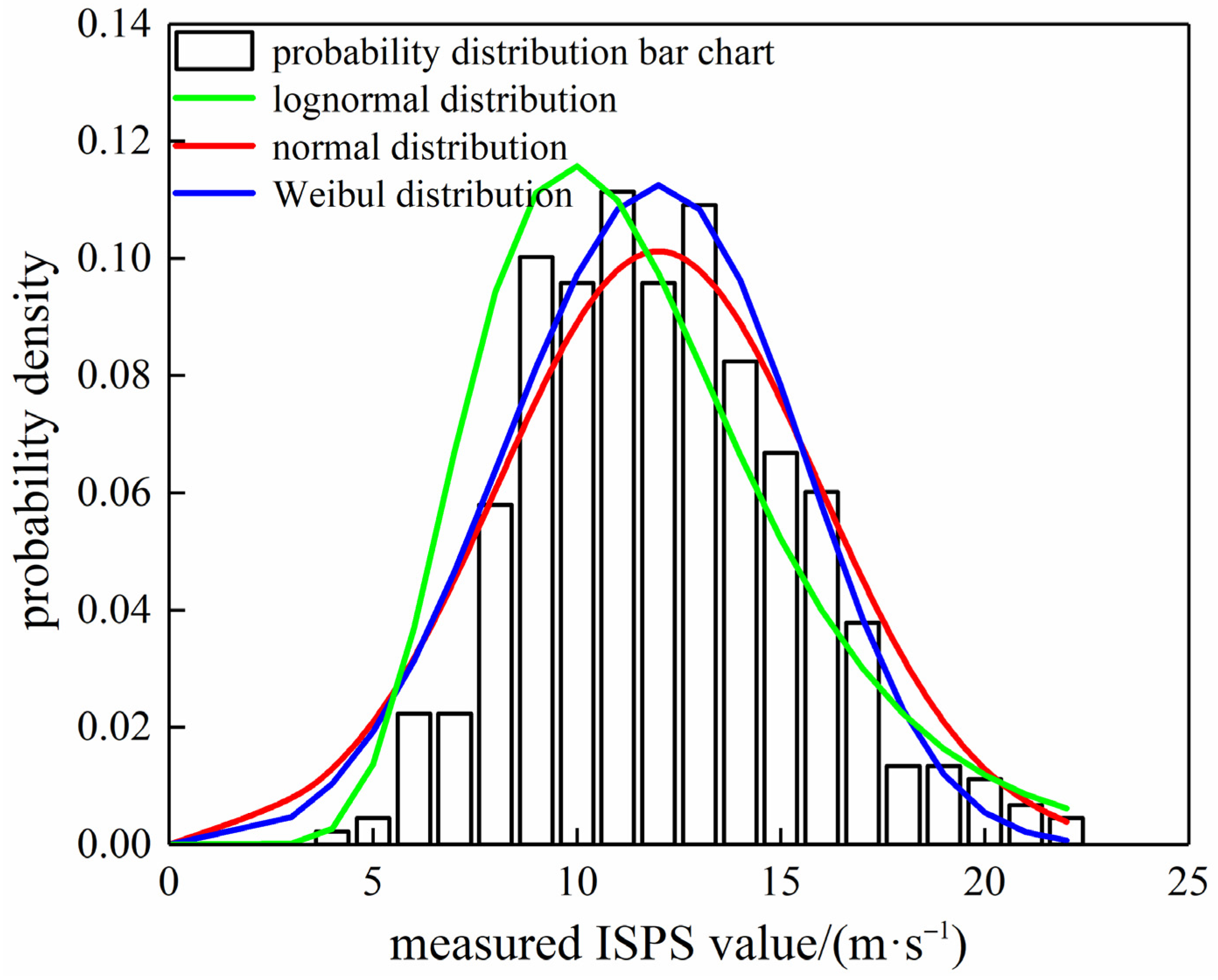
To ensure consistency of the distribution between the PISPS generated by Monte–Carlo simulation and the measured ISPS, it is firstly essential to fit the distribution of measured ISPS. According to the relevant literature [15,16], the normal distribution, lognormal distribution and Weibull distribution models are initially selected to fit the distribution of the measured ISPS. Further, the goodness-of-fit test is carried out for the three distribution models, and the best-fitting distribution model is selected by comparison. Figure 7 illustrates the fitting of the distribution of measured ISPS.
To assess the goodness-of-fit for the three distribution models, the Kolmogorov–Smirnow (K-S) test is considered [9,19]. In this test, the K-S statistic Dn is defined as follows:
D n = max F v j F 0 v j , 0 < j n
K s = n · D n
In this process, the entire population of ISPS is divided into n small intervals, and the midpoint of each interval is taken as a statistical variable. Where v j represents the j-th statistical variable, F · represents the empirical cumulative distribution function of the statistical variables. F 0 · represents a specific theoretical distribution function. And Ks represents the K-S test index. The goodness-of-fit is determined by comparing the Ks to the index limit value Kg obtained from the K-S test table. For example, given a certain confidence level, when Ks < Kg, this indicates that the goodness-of-fit of the distribution model is feasible.
In addition, in order to further compare the goodness-of-fit, the fitting determination coefficients corresponding to the three distribution models are calculated, respectively, where the calculation formula of the determination coefficient R 2 is as follows:
R 2 = 1 j = 1 n v j F 0 p j 2 j = 1 n v j v ¯ 2
where F 0 · represents the inverse function of F 0 · . v ¯ represents the mean value of all statistical variables. R 2 represents the determination coefficient and, when the value of R 2 is closer to 1, the goodness-of-fit is higher.
From the above calculation, the determined K-S test index Ks values and the determination coefficient R 2 values are as shown in the Table 1.
As can be seen from Table 1, the K-S test index Ks corresponding to the three distribution models are all less than Kg, while the Kg is 1.35 with a 5% confidence level, and the Ks value corresponding to the normal distribution is the smallest. At the same time, the value of R 2 corresponding to the normal distribution is closest to 1. This shows that the normal distribution fits the measured ISPS relatively well. In Table 1, the distribution parameters can be directly fitted by using the relevant analysis software according to the wind speed data. In addition, the moment estimation method and the maximum likelihood estimation method are used to estimate, and the final distribution parameters are determined by comparison and adjustment, which will not be described here.

3.2. Generation of the PISPS

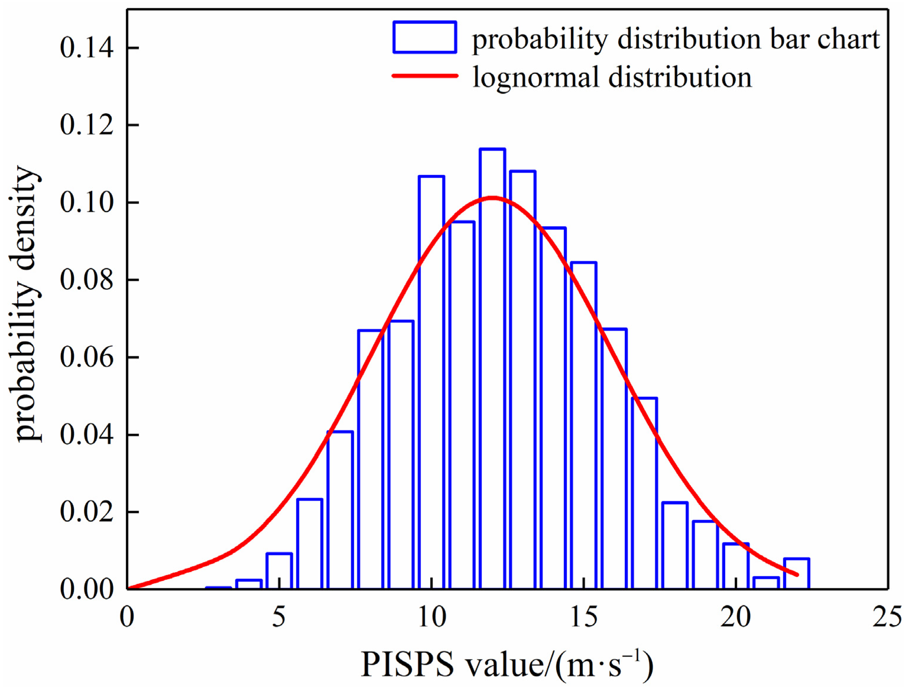
According to the normal distribution of measured ISPS, Monte–Carlo simulation is used to randomly generate PISPS with the same distribution. To meet the sample number requirements for RPWS prediction using annual maximum wind speed samples, 100 years of PISPS are generated by simulation. Therefore, given a 4-day duration for each independent storm event, a total of 100 sets of PISPS are obtained by simulation with 91 independent storm events per year as a group. From each set of samples, the maximum value is selected as the annual maximum wind speed sample. In this process, firstly, 9100 pseudo-random numbers in the [0,1] interval are generated using the multiplicative congruential method. Then, the PISPS values that completely obey the normal distribution are obtained by using the inverse transformation of the normal distribution function. The calculation process is detailed in Equation (5). At the same time, it should be noted that the distribution of the measured ISPS has a certain deviation from the normal distribution. Therefore, in order to fully ensure the consistency between the simulated PISPS and the measured ISPS, the PISPS values that completely obey the normal distribution are treated with corresponding deviation, and the final simulated generated PISPS are shown in Figure 8. Figure 9 shows the probability density distribution of PISPS.
The probability density function of the normal distribution and its inverse cumulative distribution function are as follows:
x i = ψ 1 p i
where ψ · represents the cumulative distribution function of the normal distribution. ψ 1 · represents the inverse function of ψ · . p i denotes the i-th pseudo-random number. x i denotes the value of PISPS produced by substituting p i into ψ 1 · .
As shown in Figure 9, the distribution of PISPS generated by Monte–Carlo simulation is similar to that of the measured ISPS (Figure 7). Thus, the consistency between PISPS and ISPS is ensured as much as possible to make up for the shortage of measured wind speed samples.

4. RPWS Prediction for the Whole Wind Direction

Given the PISPS generated using the Monte–Carlo simulation method as described above, annual maximum wind speed samples are extracted for RPWS prediction. Relevant research [15] has shown that the accuracy of RPWS results predicted using EVT I and EVT III distribution models is relatively high for wind speed samples following the normal distribution. Therefore, according to the PISPS generated by simulation, the EVT I and EVT III distribution models are used to predict the RPWS of the whole wind direction, respectively. In addition, in order to illustrate the effectiveness of the RPWS results predicted by PISPS, the over-threshold independent storm peak samples (OISPS) are extracted from the original measured ISPS and the GPDM is used to predict RPWS. The following explanation focuses on the results of RPWS prediction for the whole wind direction at a height of 200 m.

4.1. RPWS Prediction Based on PISPS

(1)
EVT I distribution model
The EVT I distribution model with two parameters is expressed as follows:
F 1 V ; a 1 , b 1 = exp exp ( V b 1 a 1 ) , < V < +
where F 1 · represents the probability distribution function for the EVT I model. V represents the extreme wind speed variable. a 1 and b 1 represent the scale parameter and the position parameter, respectively. When the sample size is sufficient, the moment method can be used to determine the distribution parameters of EVT I distribution model. The moment estimation method is as follows:
X ¯ = b ^ 1 + Γ · a ^ 1 a ^ 1 = π 6 σ X
where X represents the annual maximum wind speed variable. X ¯ and σ X represent the mean and standard deviation of X . a ^ 1 and b ^ 1 are the estimated values of a 1 and b 1 , respectively. Γ is Euler’s constant, usually set to 0.5772.
(2)
EVT III distribution model
The EVT III distribution model with three parameters is expressed as follows:
F 3 V ; a 3 , b 3 , γ = exp ( V b 3 a 3 ) γ , V < b 3
where F 3 · represents the probability distribution function for the EVT III model. a 3 represents the scale parameter. b 3 represents the position parameter. γ represents the shape parameter. The maximum likelihood estimation method is usually used to determine the distribution parameters in the EVT III distribution model. And the maximum likelihood estimation method is as follows:
i = 1 N b ^ 3 X i γ ^ 1 γ ^ 1 N γ ^ i = 1 N b ^ 3 X i γ ^ · i = 1 N b ^ 3 X i 1 = 0
a ^ 3 = 1 N · i = 1 N b ^ 3 X i γ ^ 1 γ ^
where X i is the ith order statistic of the annual maximum wind speed samples. a ^ 3 , b ^ 3 and γ ^ are the estimated values of the scale parameter a 3 , position parameter b 3 and shape parameter γ , respectively. In this process, in order to ensure the parameter validity of maximum likelihood estimation, γ ^ value is determined by stepwise iteration. At the same time, the probability curve correlation coefficient method is used to determine the optimal γ ^ . And the definition of the probability curve correlation coefficient S is given in Equation (11).
S = i = 1 N X i X ¯ · M 1 P i M 1 P i ¯ i = 1 N X i X ¯ 2 · i = 1 N M 1 P i M 1 P i ¯ 2
where P i is the empirical distribution probability of the ith order statistic X i . M 1 · represents the inverse function of a certain extreme value distribution model and M 1 · ¯ is the mean value of all M 1 · values. Here, the probability curve correlation coefficient S is a function with respect to the shape parameter variable γ , and k = d S / d γ represents the slope of the probability correlation coefficient curve. When γ = γ ^ , if k 0.01 , then γ ^ is the optimal estimate value of γ .
In summary, the distribution parameters corresponding to the EVT I and EVT III distribution models are shown in Table 2.

4.2. RPWS Prediction Based on the Measured OISPS

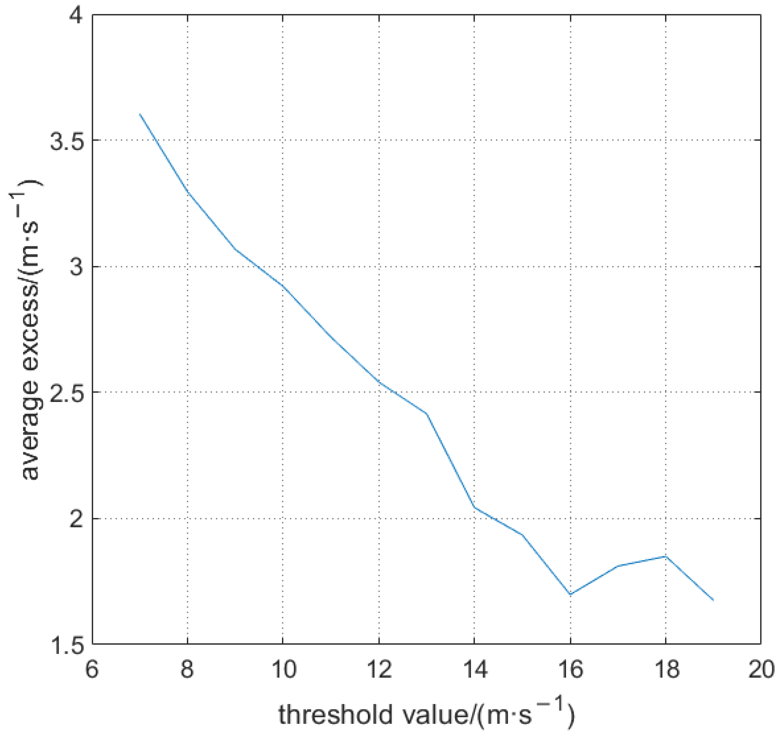
On basis of the measured ISPS (as shown in Figure 6), an appropriate threshold is selected for extracting OISPS. The threshold can be determined using the average residual life plot [9]. In this process, the threshold interval that may contain the optimal threshold is preliminarily determined according to the measured daily maximum wind speed samples. Subsequently, different thresholds are used to calculate the average excesses values of wind speed samples, and an average residual life plot is generated, as shown in Figure 10. In Figure 10, it can be observed that, when the threshold is less than 16 m/s, the average excess plot generally shows a linear trend, whereas, when the threshold exceeds 16 m/s, the plot exhibits significant fluctuations and is no longer linear. Therefore, 16 m/s is chosen as the optimal threshold for further screening and extraction of OISPS. Some values of the OISPS are shown in Figure 11.
When performing RPWS prediction using OISPS, the Generalized Pareto Distribution Model (GPDM) is commonly used for analysis. The distribution function expression of the GPDM is as follows:
F G V ; μ 0 , σ 0 , γ = 1 1 + γ V μ 0 σ 0 1 / γ
where F G · represents the probability distribution function of the GPDM. μ 0 , σ 0 and γ represent the threshold, the scale parameter and the shape parameter, respectively. In this process, the distribution parameters are estimated using the maximum likelihood estimation method, and the detailed analysis process is described in Section 4.1 (2). Thus, μ 0 = 16 , σ 0 = 1.89 , and γ = 0.032 . Additionally, there is a corresponding relationship [22,23] between F G · determined by the fitting of OISPS and the annual extreme value probability distribution function F y , and the relationship is as follows:
F y = F G · g
where g represents the average number of OISPS contained in each year.

4.3. RPWS Prediction Results for the Whole Wind Direction

The 50-year RPWS prediction values are calculated, respectively, according to the PISPS determined by the Monte–Carlo simulation and the OISPS extracted from the measured wind speed samples, and the RPWS results are shown in Figure 12. To facilitate a comparison with the specified values in the code, the basic wind pressure corresponding to the 50-year return period in the Beijing area, as defined in the code, is further converted into the RPWS design value under the actual terrain conditions. The formula for converting the basic wind pressure to RPWS design value is as follows:
V h , 50 = 2 · W 0 · H B 10 2 α B · h H D 2 α D ρ
where V h , 50 represents the converted 50-year RPWS design value at height h. W 0 represents the basic wind pressure value corresponding to the 50-year return period in the code. H B and H D represent the gradient wind heights corresponding to Class B and Class D terrains, respectively, as per the code. The code specifies that H B = 350   m and H D = 550   m . α B and α D represent the wind profile indexes corresponding to Class B and Class D terrains, respectively. The standards specify that α B = 0.15 , while the value for α D based on the wind speed profile index fitting from measured wind speed data (as seen in Figure 3) is taken as 0.32. ρ represents air density, which is generally taken as 1.25 kg/m3.
As can be seen from Figure 12, according to the PISPS generated by Monte–Carlo simulation, the 50-year RPWS prediction results calculated using the EVT I and EVT III distribution models are 31.21 m/s and 30.11 m/s, respectively, with a relative deviation of about 3.5%. Meanwhile, according to the measured OISPS, the RPWS value predicted by the GPDM is 29.25 m/s and the relative deviations from the RPWS value predicted by the EVT I and EVT III distribution models are about 6.7% and 2.9%, respectively. Meanwhile, compared to the RPWS design value ( V h , 50 = 33.1   m / s ) converted from the code, all RPWS prediction results fall within the envelope range of the design value.

5. RPWS Prediction Considering Wind Direction

In the previous sections, the RPWS predictions are made for the whole wind direction using different extreme value distribution models based on both PISPS and OISPS, and these prediction results are compared and analyzed. According to the RPWS results in the whole wind direction, further investigations are conducted to explore the distribution of RPWS in different wind directions within Beijing city. Thus, the traditional Cook method is used to predict the RPWS considering wind direction according to the measured wind speed samples [24,25,26].

5.1. Analysis of Wind Speed–Direction Distribution

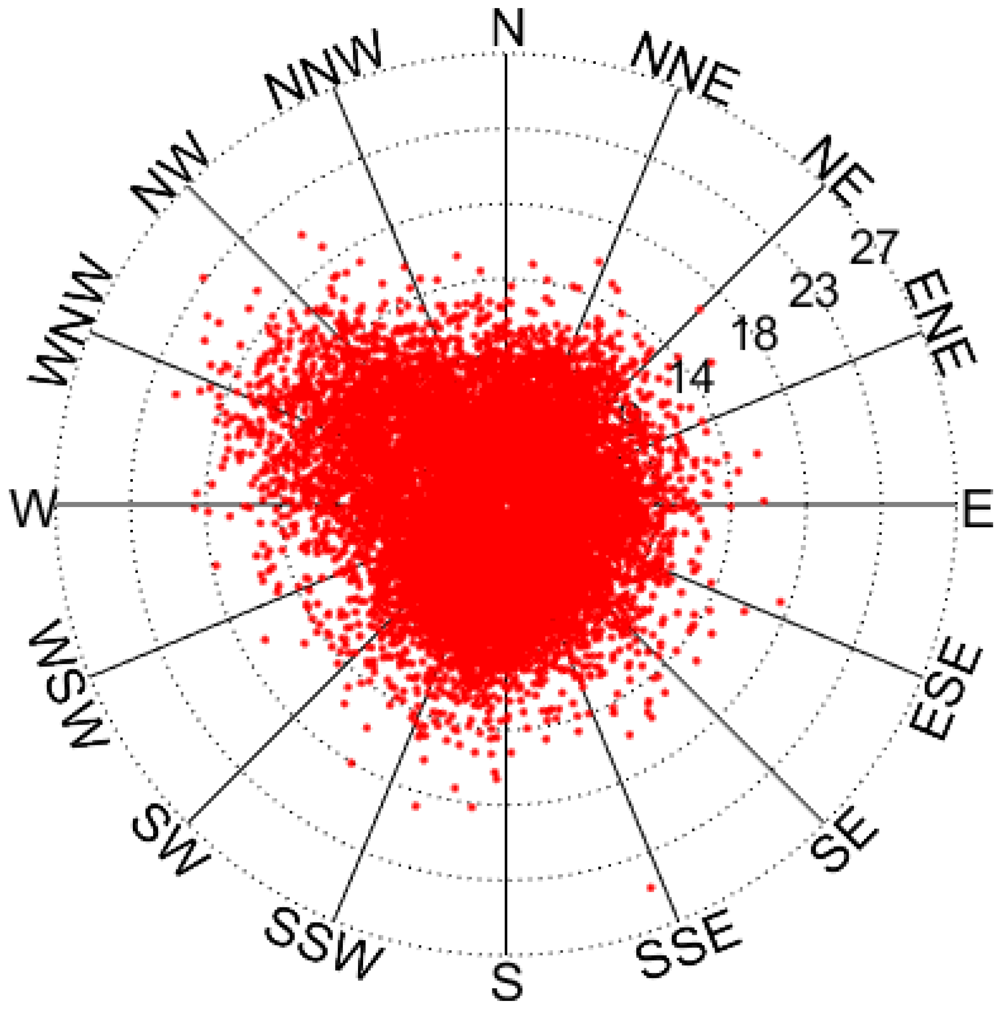
For the measured 10 min average wind speed samples, the different 10 min average wind speed data correspond to different wind directions. On basis of the measured 10 min average wind speed samples at a height of 200 m, the daily maximum wind speed samples are statistically extracted for various wind directions. In this process, it is essential to note that the number of the measured wind speed samples is small if the daily maximum wind speed samples are extracted from the 10 min average wind speed data directly, and then these daily maximum wind speed samples are classified and distributed according to the wind direction of the samples with each daily maximum wind speed sample corresponding to a single wind direction, and thus it may result in a situation where there are very few samples in some wind directions, making it insufficient for RPWS prediction. Therefore, in order to maximize the sample number of the daily maximum wind speed in each wind direction as much as possible, firstly, the 10 min average wind speed data are distributed to the corresponding wind directions in this paper, so that the 10 min average wind speed data in the same day can be distributed in different wind directions. Subsequently, the corresponding daily maximum wind speed samples are extracted in each wind direction, respectively, so as to realize the increase in the daily maximum wind speed sample number in each wind direction. The distribution of daily maximum wind speed samples for each wind direction is shown in Figure 13. In Figure 13, the red scatter points indicate the daily maximum wind speed samples.
In Figure 13, the dominant wind direction is the northwest wind direction, and the distribution of larger wind speed sample values is concentrated in this wind direction, so the wind speed–direction distribution is consistent with the characteristics of monsoon climate in Beijing.

5.2. RPWS Prediction for Each Wind Direction Using the Cook Method

According to the traditional Cook prediction method, it was assumed that the RPWS of different wind directions change in the same proportion, that is, the distribution shape of the RPWS rose plot remains basically unchanged. Thus, RPWS values for different wind directions are determined using a specific scale factor, and the detailed analysis steps can be found in Quan et al. [26]. In this paper, the GPDM is used for the RPWS prediction analysis according to the OISPS of each wind direction. In the process of analysis, it was initially assumed that wind speeds for different wind directions are entirely positively correlated. Thus, for an R-year return period, the non-exceedance probability of the RPWS is equal for the whole wind direction and each wind direction.
F V v = F V z v d z = 1 1 / R
F V v = P max ( V d 1 , V d 2 , , V d 16 ) v F V z v d z = = P V d z v d z ; z = 1 , 2 , 3 , 16
where F V · and F V z · represent the extreme probability distribution functions for the whole wind direction and the zth wind direction, respectively. v and v d z represent the RPWS variables for the whole wind direction and the zth wind direction, respectively. V d z represents the maximum wind speed sample for the zth wind direction.
It is worth discussing that the daily maximum wind speed samples in each wind direction are extracted and obtained from the 10 min average wind speed data distributed to each wind direction, so the daily maximum wind speed sample values in each wind direction will be relatively small as a whole. But, in the process of RPWS prediction of each wind direction by Cook method, the amplitude of the daily maximum wind speed samples of each wind direction will be adjusted according to the ratio of the preliminary RPWS prediction value of the whole wind direction to that of each wind direction, so the influence of the small initial daily maximum wind speed sample value on the final RPWS prediction result of each wind direction will be eliminated.

5.3. Analysis of RPWS Prediction Results

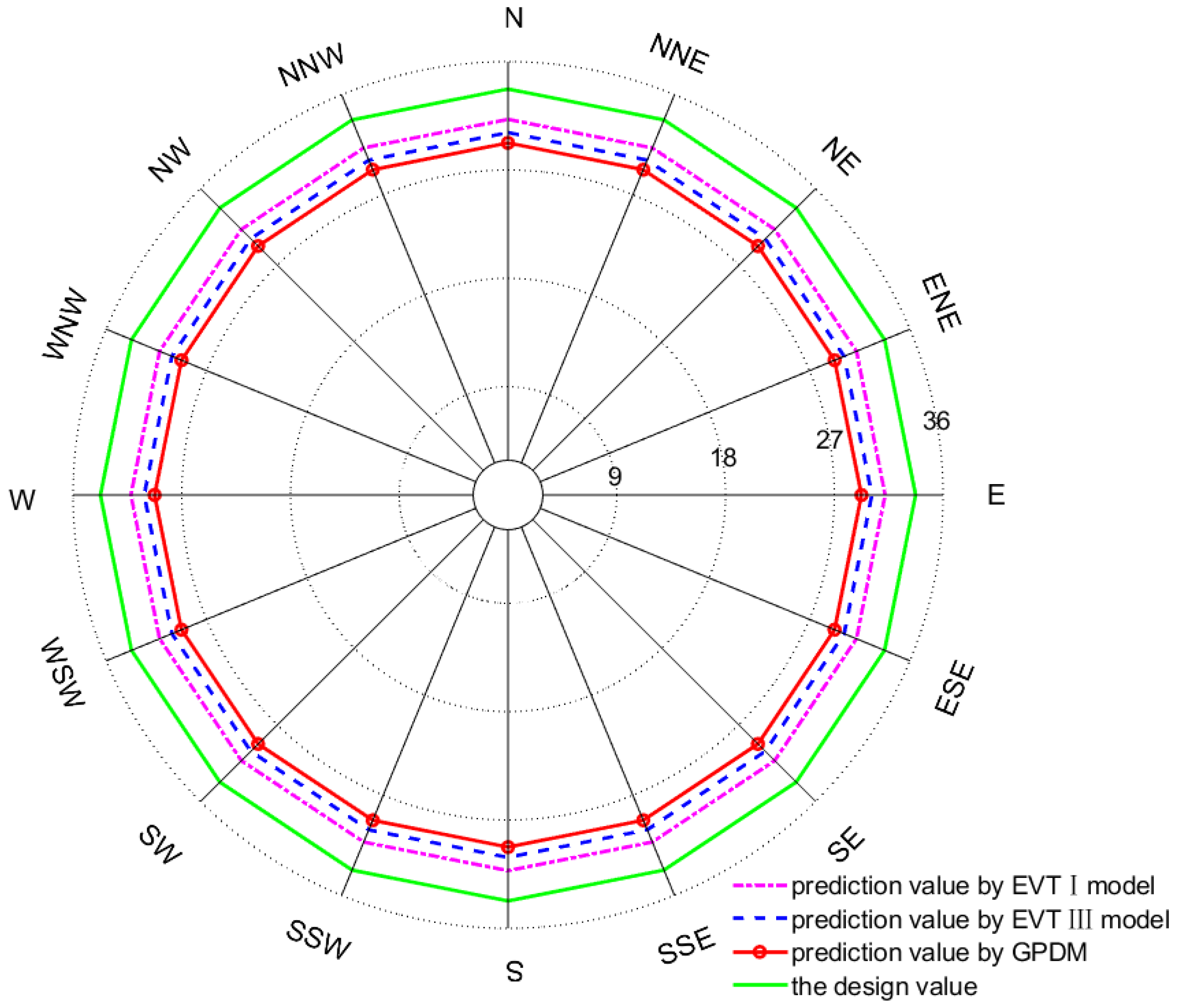
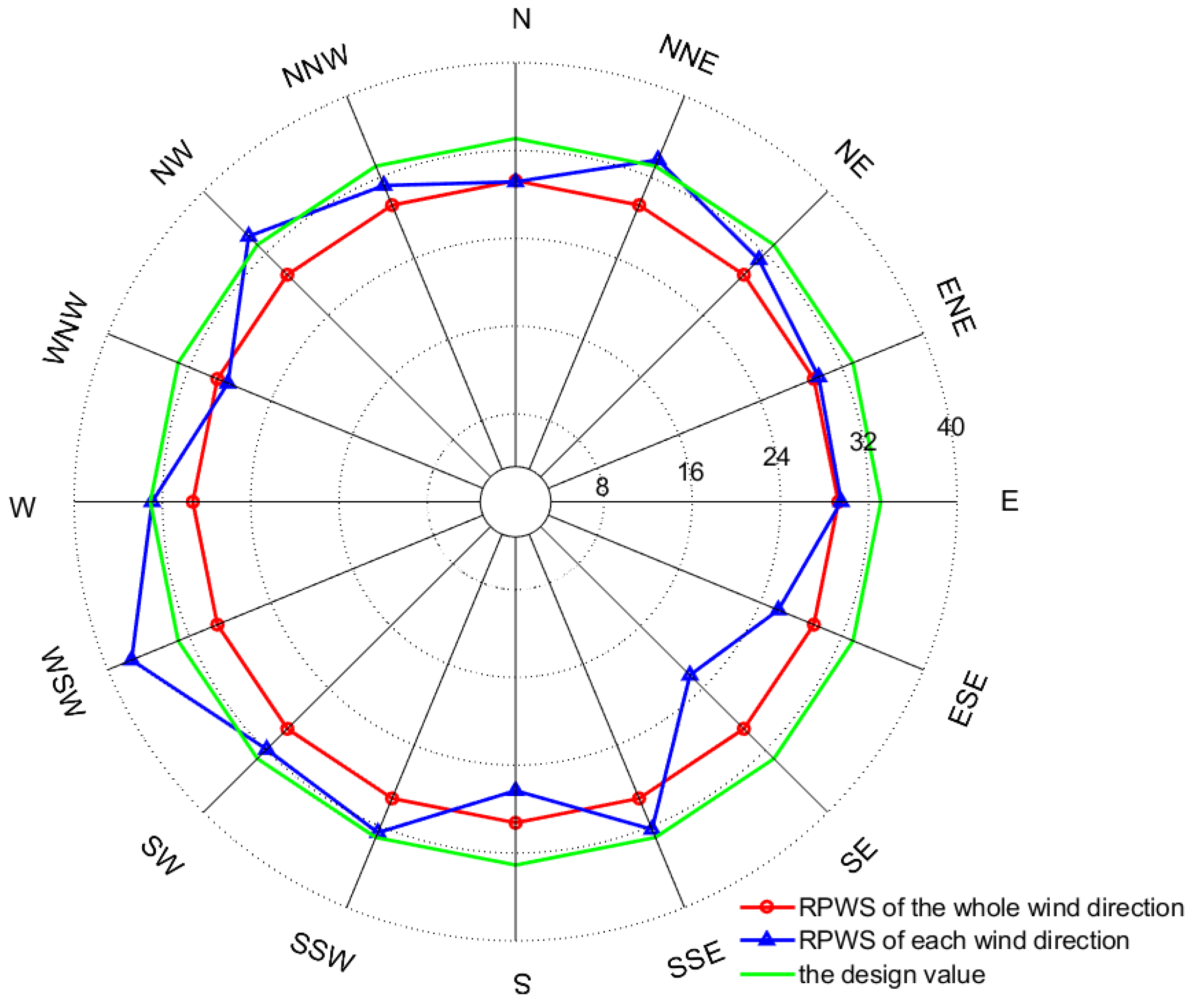
Given the Cook method, the 50-year RPWS v d z of each wind direction at a height of 200 m is calculated. And the RPWS values are compared with the RPWS prediction value ( v = 29.25   m / s ) of the whole wind direction and the design value ( V h , 50 = 33.1   m / s ) in code. The comparison of the 50-year RPWS prediction results is shown in Figure 14. And the relative deviations between v d z and v , V h , 50 are further calculated as follows:
e = v d z v v
e = v d z V h , 50 V h , 50
where e represents the absolute value of the relative deviation between v d z and v . e represents the absolute value of the relative deviation between v d z and V h , 50 . And the relative deviation results are shown in the Table 3.
In Figure 14, it is evident that the design value 33.1 m/s is basically sufficient to envelop the RPWS prediction value of each wind direction. However, in the case of southwest, northwest and northeast wind directions, higher wind speed values are encountered, and the maximum RPWS occurs in the west-southwest wind direction with 37.66 m/s. Further, compared with the predicted value of the whole wind direction, the mean relative deviation of the RPWS prediction values between each wind direction and the whole wind direction is approximately 10.6%.

6. Discussion and Conclusions

According to the short-term measured wind speed records, the Monte–Carlo simulation method is used to generate pseudo-independent storm peak samples (PISPS), and the over-threshold independent storm peak samples (OISPS) are extracted from the measured samples. Thus, the EVT I, EVT III and GPD distribution models are used to predict the return period wind speed (RPWS) of the whole wind direction, respectively. Furthermore, the RPWS of each wind direction is predicted by the traditional Cook method and compared with the prediction values of the whole wind direction and the design values of code. In the analysis process, the main shortcomings are as follows: on the one hand, the number of the measured wind speed sample is small, which will lead to large deviations in the RPWS prediction results, especially for the RPWS prediction result of each wind direction. On the other hand, when the Cook method is applied to predict the RPWS of each wind direction, it is assumed that the non-exceeding probability of the RPWS of each wind direction is equal but, in fact, the RPWS of each wind direction is partially correlated, so the correlation analysis of the RPWS for different wind directions needs to be further studied.
In this paper, the results show that, according to the PISPS generated by Monte–Carlo simulation, the RPWS of the whole wind direction predicted by the EVT I and EVT III distribution models are basically close to each other, and the relative deviation is about 3.5%. In addition, for the measured OISPS, the RPWS value predicted by the GPDM is also close to those predicted by the EVT I and EVT III distribution models, and the relative deviations are about 6.7% and 2.9%, respectively. Therefore, the relative errors of the RPWS prediction results corresponding to the simulated PISPS and the measured OISPS are kept within 10%, which indicates that it is feasible to make up for the lack of measured samples by the Monte–Carlo simulation method. In addition, the RPWS results of the whole wind direction predicted by the GPD model are slightly larger, mainly because the number of measured OISPS is small and the RPWS prediction results are greatly affected by larger wind speed samples.
The mean relative deviation of prediction values is about 10.6% between the RPWS of each wind direction and the RPWS of the whole wind direction. And the predicted values in the west-southwest, northwest, and north-northeast wind directions are relatively large and exceed the code design values. However, the predicted values of other wind directions basically remain within the envelope range of the design value. Therefore, when carrying out the wind resistance design of building structures, it is necessary to consider the reduction or expansion of wind speed from different wind directions.

Author Contributions

Conceptualization, W.C. and Y.T.; methodology, W.C. and Y.T.; software, W.C.; validation, Y.T.; formal analysis, Y.T.; investigation, W.C.; resources, Y.T.; data curation, Y.T.; writing—original draft preparation, W.C.; writing—review and editing, Y.T.; visualization, W.C.; supervision, Y.T.; project administration, Y.T.; funding acquisition, Y.T. All authors have read and agreed to the published version of the manuscript.

Funding

This research was funded by the National Natural Science Foundation of China grant number No. 51878040 and No. 51720105005.

Institutional Review Board Statement

Not applicable.

Informed Consent Statement

Not applicable.

Data Availability Statement

Data available on request due to restrictions eg privacy or ethical. The data presented in this study are available on request from the corresponding author. The data are not publicly available due to data confidentiality.

Conflicts of Interest

The authors declare no conflict of interest.

References

  1. Ministry of Housing and Urban-Rural Development of the People’s Republic of China. Load Code for the Design of Building Structures: GB 50009—2012; China Architecture & Building Press: Beijing, China, 2012.
  2. Wang, B.; Dong, Y.; Dong, L. Calculation of basic wind pressure based on short-term wind speed data. J. Jilin Univ. (Eng. Technol. Ed.) 2020, 50, 1739–1746. [Google Scholar]
  3. Cook, N.J. Towards better estimation of extreme winds. J. Wind. Eng. Ind. Aerodyn. 1982, 9, 295–323. [Google Scholar] [CrossRef]
  4. Luo, Y.; Zhu, L.S. A new model of peaks over threshold for multivariate extremes. China Ocean. Eng. 2014, 28, 761–776. [Google Scholar] [CrossRef]
  5. Duthinh, D.; Pintar, A.L.; Simiu, E. Estimating peaks of stationary random processes: A peaks-over-threshold approach. ASCE-ASME J. Risk Uncertain. Eng. Syst. Part A Civ. Eng. 2017, 3, 04017028. [Google Scholar]
  6. Harris, R.I. Improvements to the Method of Independent Storms. J. Wind. Eng. Ind. Aerodyn. 1999, 80, 1–30. [Google Scholar] [CrossRef]
  7. Luo, Y.; Huang, G.-Q.; Chen, B.-Z.; Liu, W.-Z.; Li, M.-S.; Liao, H.-L. Design wind speed estimation for puli bridge based on short-term measured data. Eng. Mech. 2018, 35, 74–82. [Google Scholar]
  8. Di, W.; Yue, W.; Qingshan, Y.; Long, C. Improved method of independent storms for extreme value estimation of non-Gaussian wind pressure. J. Build. Struct. 2014, 35, 151–156. [Google Scholar]
  9. Shi, D. Practical Statistical Methods for Extremes; Tianjin Science and Technology Press: Tianjin, China, 2006. [Google Scholar]
  10. Wang, J.; Qin, S.; Jin, S.; Wu, J. Estimation methods review and analysis of offshore extreme wind speeds and wind energy resources. Renew. Sustain. Energy Rev. 2015, 42, 26–42. [Google Scholar] [CrossRef]
  11. An, Y.; Pandey, M.D. A comparison of methods of extreme wind speed estimation. J. Wind. Eng. Ind. Aerodyn. 2005, 93, 535–545. [Google Scholar] [CrossRef]
  12. D’Amico, G.; Petroni, F.; Prattico, F. Wind speed prediction for wind farm applications by extreme value theory and copulas. J. Wind. Eng. Ind. Aerodyn. 2015, 145, 229–236. [Google Scholar]
  13. Duan, Z.; Ou, J.; Zhou, D. The optimal probabilistic distribution for extreme wind speed. China Civ. Eng. J. 2002, 35, 11–16. [Google Scholar]
  14. Zhao, L.; Ge, Y.; Xiang, H. Optimization strategy of extreme wind speed fitting. J. Tongji Univ. (Nat. Sci.) 2003, 31, 383–388. [Google Scholar]
  15. Lu, A.; Zhao, L.; Guo, Z.; Ge, Y. A comparative study of extreme value distribution and parameter estimation based on the Monte Carlo method. J. Harbin Inst. Technol. 2013, 45, 88–95. [Google Scholar]
  16. Morgan, E.C.; Lackner, M.; Vogel, R.M.; Baise, L.G. Probability distributions for offshore wind speeds. Energy Convers. Manag. 2011, 52, 15–26. [Google Scholar] [CrossRef]
  17. Patlakas, P.; Galanis, G.; Barranger, N.; Kallos, G. Extreme wind events in a complex maritime environment: Ways of quantification. J. Wind. Eng. Ind. Aerodyn. 2016, 149, 89–101. [Google Scholar]
  18. Chen, Z.; Guan, Q. Simulating of asymptotic distributions of extreme wind speed in Chongqing using short-term wind speed records. J. Chongqing Univ. 2006, 29, 88–92. [Google Scholar]
  19. Gugliani, G.K.; Sarkar, A.; Bhadani, S.; Mandal, S. A novel approach for accurate assessment of design wind speed for variable wind climate. KSCE J. Civ. Eng. 2019, 23, 608–623. [Google Scholar]
  20. Li, B.; Li, C.; Yang, Q.; Tian, Y.; Zhang, X. Full-scale wind speed spectra of 5 Year time series in urban boundary layer observed on a 325 m meteorological tower. J. Wind. Eng. Ind. Aerodyn. 2021, 218, 104791. [Google Scholar] [CrossRef]
  21. Simiu, E.; Heckert, N.A. Extreme wind distribution tails: A peaks over threshold approach. J. Struct. Eng. 1996, 122, 539–547. [Google Scholar] [CrossRef]
  22. ESDU (Engineering Science Data Unit). World-Wide Extreme Wind Speeds: Part 1: Origins and Methods of Analysis; HIS (Information Handling Service): London, UK, 2012. [Google Scholar]
  23. Cook, N.J. Designers Guide to Wind Loading of Building Structures. Part 1: Background, Damage Survey, Wind Data and Structural Classification; Building Research Establishment Report; Butterworths: London, UK, 1986; pp. 99–116. [Google Scholar]
  24. Cook, N.J. Note on directional and seasonal assessment of extreme winds for design. J. Wind. Eng. Ind. Aerodyn. 1983, 12, 365–372. [Google Scholar]
  25. Cook, N.J.; Miller, C.A. Further note on directional assessment of extreme winds for design. J. Wind. Eng. Ind. Aerodyn. 1999, 79, 201–208. [Google Scholar] [CrossRef]
  26. Quan, Y.; Liu, L.; Gu, M. Improvement of Cook method considering directional extreme wind speed. J. Tongji Univ. (Nat. Sci.) 2015, 43, 189–192. [Google Scholar]
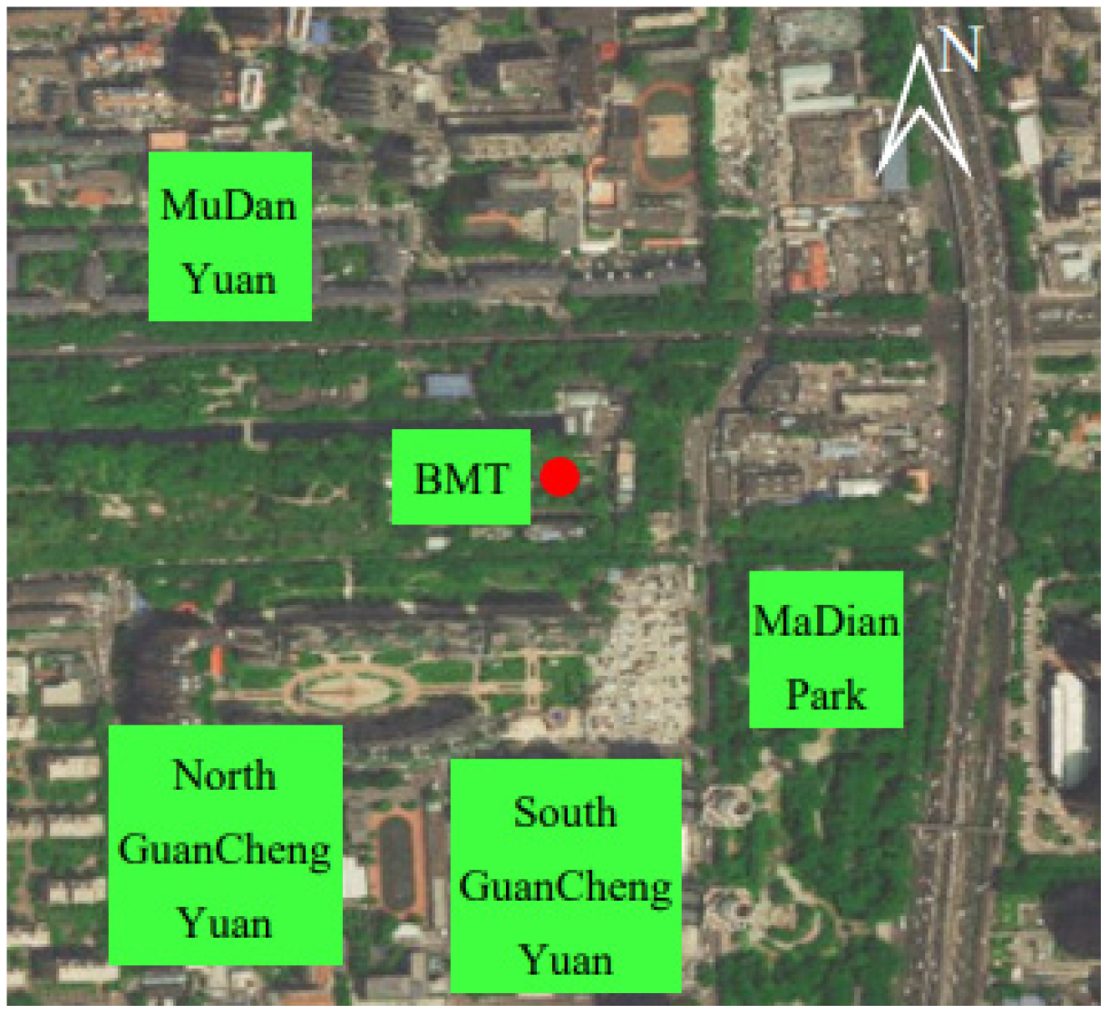
Figure 1. Location of Beijing Meteorological Tower.
Atmosphere 15 00159 g001
Figure 2. Measured wind speed records in 2015.
Atmosphere 15 00159 g002
Figure 3. Wind profile index.
Atmosphere 15 00159 g003
Figure 4. Sample time history of daily maximum wind speed from 2013 to 2017.
Atmosphere 15 00159 g004
Figure 5. Autocorrelation coefficient curve.
Atmosphere 15 00159 g005
Figure 6. Measured ISPS.
Atmosphere 15 00159 g006
Figure 7. Fitting distribution of the measured ISPS.
Atmosphere 15 00159 g007
Figure 8. Partial PISPS.
Atmosphere 15 00159 g008
Figure 9. The probability distribution of PISPS.
Atmosphere 15 00159 g009
Figure 10. Plot of the average residual lifetime.
Atmosphere 15 00159 g010
Figure 11. Measured OISPS.
Atmosphere 15 00159 g011
Figure 12. The RPWS results of the whole wind direction (m·s−1).
Atmosphere 15 00159 g012
Figure 13. Wind speed–direction distribution (m·s−1).
Atmosphere 15 00159 g013
Figure 14. Comparison of the 50-year RPWS prediction results (m·s−1).
Atmosphere 15 00159 g014
Table 1. The Ks and R 2 values corresponding to the three distribution models.
ModelPosition
Parameters
Scale
Parameters
Shape
Parameters
KsR2
lognormal2.40.330.890.80
normal123.90.790.85
Weibull133.830.960.79
Table 2. The distribution parameters corresponding to the EVT I and EVT III models.
ModelPosition ParametersScale ParametersShape Parameters
EVT I22.042.35
EVT III38.9416.766.09
Table 3. The 50-year RPWS value of each wind direction and the relative deviation.
Wind Direction v d z /(m·s−1) e * (%) e (%)
N29.150.340.3
NNE33.7215.2813.5
NE31.196.625.85
ENE29.731.631.44
E29.500.860.76
ESE25.7711.910.52
SE22.3423.6320.88
SSE32.3110.459.23
S26.3210.028.86
SSW32.6211.5410.2
SW31.909.078.01
WSW37.6628.7625.42
W32.9412.6111.14
WNW28.223.533.12
NW34.2016.9414.97
NNW31.196.635.86
Mean30.5510.69.4
Disclaimer/Publisher’s Note: The statements, opinions and data contained in all publications are solely those of the individual author(s) and contributor(s) and not of MDPI and/or the editor(s). MDPI and/or the editor(s) disclaim responsibility for any injury to people or property resulting from any ideas, methods, instructions or products referred to in the content.