Exploring Urban XCO₂ Patterns Using PRISMA Satellite: A Case Study in Shanghai

Abstract

As global warming intensifies, monitoring carbon dioxide (CO₂) has increasingly become a focal point of research. Investigating urban XCO₂ emission systems holds paramount importance, given the pivotal role of cities as major contributors to carbon emissions. Consequently, this study centers on urban locales, employing Shanghai as a case study for a comprehensive evaluation of regional XCO₂ levels. We utilized high spatial resolution imagery from the PRecursore IperSpettrale della Missione Applicativa (PRISMA) satellite to conduct an XCO₂ assessment over the Baoshan District with a 30 m spatial resolution from April 2021 to October 2022. Our XCO₂ analysis was conducted in two steps. Firstly, we conducted a sensitivity analysis on key parameters in the inversion process, where cloud cover severely interfered with inversion accuracy. Therefore, we developed the Fmask 4.0 cloud removal and iterative maximum a posteriori differential optical absorption spectroscopy (FIMAP-DOAS) algorithm. This novel integration eliminated cloud interference during the inversion process, achieving high-precision CO₂ detection in the region. Secondly, we compared the XCO₂ of the region with Level-2 data from carbon monitoring satellites such as OCO-2. The comparison results showed a strong consistency, with a root mean squared error (RMSE) of 0.75 ppm for Shanghai XCO₂ data obtained from the PRISMA satellite compared to OCO-2 Level-2 data and an RMSE of 1.49 ppm compared to OCO-3. This study successfully established a high-accuracy and high-spatial-resolution XCO₂ satellite monitoring system for the Shanghai area. The efficacy of the FIMAP-DOAS algorithm has been demonstrated in CO₂ monitoring and inversion within urban environments, with potential applicability to other cities.

1. Introduction

The Sixth Assessment Report of the Intergovernmental Panel on Climate Change (IPCC) reported that ‘In 2019, atmospheric CO₂ concentrations (410 parts per million) were higher than at any time in at least 2 million years [1]’. The global warming caused by CO₂ is an environmental issue that cannot be ignored [2]. The Copenhagen Agreement emphasized that if left unchecked, global temperatures will rise by six degrees Celsius in the next century. More than 100 nations committed to reducing greenhouse gas emissions in 2015 by signing the Paris Agreement [3]. The Chinese government said that it will attain the carbon peak by 2030 and achieve carbon neutrality by 2060 during the 75th United Nations General Assembly in 2020 [4]. Developing effective strategies to minimize carbon emissions requires a systematic analysis of the temporal and geographical distribution of CO₂ in cities over an extended period.

Satellite remote sensing offers significant advantages, including broad coverage and an extended time series, making it a valuable tool for monitoring CO₂ [5]. This technology enables the continuous monitoring of XCO₂ in a given region. Currently, researchers employ carbon satellites for the prolonged tracking of XCO₂ in specific regions, including Japan’s GOSAT [6], GOSAT-2 [7], OCO-2 [8], its next-generation OCO-3 [9] satellites, and China’s carbon satellite (TanSat) [10]. Various countries’ researchers have developed standard inversion algorithms, such as NIES [11], ACOS [12,13], RemoTec [14], and IAPCAS [15], to retrieve XCO₂ data from these satellites.

However, the spatial resolution of these satellites is relatively rough [16,17], and there are certain limitations in local area inversion and point source scale monitoring of XCO₂. Currently, some researchers have solved this problem through spatial interpolation [18,19] and multi-satellite spatiotemporal data fusion [20,21], but these methods perform better at large spatial scales.

With its 30 m spatial resolution, PRecursore IperSpettrale della Missione Applicativa (PRISMA) satellite data provide immediate and effective solutions to challenges faced by carbon satellites in addressing local point sources and monitoring XCO₂ [22]. Launched in 2019 as a hyperspectral satellite, PRISMA holds a unique advantage in urban XCO₂ monitoring due to its extensive spectral coverage. In recent years, researchers have begun to leverage data from the PRISMA satellite for the inversion of greenhouse gas concentrations. Acito, N., et al. [23] developed a matched filter approach for the rapid inversion of CO₂ concentrations, while Kai, Q., et al. [24] utilized PRISMA satellite data for the continuous tracking and monitoring of CH₄ in coal development regions. Additionally, PRISMA data can fill detection gaps in other carbon satellites. Satellites like GOSAT and TanSat [6,10], equipped with cloud and aerosol imagers, facilitate efficient cloud layer screening and error mitigation. The OCO series of carbon satellites can utilize meteorological satellites such as MODIS for cloud removal [25]. However, the impact of clouds on XCO₂ inversion is significant, and PRISMA lacks a dedicated cloud and aerosol imager. This issue requires special attention, and potential solutions need to be explored.

This study involves conducting long-term time series inversion and monitoring for the Shanghai area. To address interference and errors introduced by cloud cover in practical applications, we developed the Fmask 4.0 cloud removal and iterative maximum a posteriori differential optical absorption spectroscopy (FIMAP-DOAS) algorithm to retrieve and monitor XCO₂ in the Shanghai region using raw spectral data from the PRISMA satellite. A reliable 30 m resolution XCO₂ satellite monitoring system has been successfully established. The paper is structured as follows: Section 1 introduces the background and objectives of the research. Section 2 briefly outlines the retrieval data materials. Section 3 offers a detailed explanation of the principles behind the FIMAP-DOAS retrieval algorithm. Section 4 discusses the results, compares them with satellite data like OCO-2, and explores limitations. Section 5 provides a summary of the main findings, emphasizing the significance of PRISMA satellite data for future research.

2. Materials

2.1. Study Area

Urban areas contribute to 71–76% of global carbon emissions, and urbanization is a primary factor in CO₂ emissions in China [26]. The pressure for carbon reduction is mainly concentrated in urban regions, making the study of carbon emissions in these areas crucial for effectively reducing global carbon emissions. Shanghai, located on the east coast of China at the mouth of the Yangtze River, serves as China’s economic hub. In 2022, it had a total population of 24.75 million and a GDP of CNY 44,652.80 billion. With a high level of urbanization at 89.6%, Shanghai is a typical megacity globally, featuring a rich industrial and shipping transportation sector. However, this high level of urbanization and industrial activity makes Shanghai a significant contributor to CO₂ emissions. Therefore, Shanghai is recognized as a crucial research area for discussions on carbon emissions and mitigation efforts [27].

Several factors led to the decision to choose Shanghai as the research’s study location. Firstly, Shanghai, being one of China’s largest cities, encompasses a variety of carbon-emission sources, including industrial activities, transportation, and energy consumption. Thus, conducting high-resolution XCO₂ monitoring and analysis in the Shanghai region yields insights into the spatial distribution and temporal variations in urban carbon emissions [28]. Secondly, Shanghai carries a significant burden of energy consumption and transportation activities, resulting in substantial carbon emissions. The FIMAP-DOAS method, coupled with PRISMA satellite data, enables the acquisition of accurate XCO₂ concentration data. This facilitates the identification and characterization of carbon-emission sources in the area, laying a scientific foundation for emission reduction plans. In addition, Shanghai is a globally integrated metropolis, making the connection between local carbon emissions and climate change crucial. By exploring XCO₂ monitoring and analysis at the urban scale, this study can contribute valuable experience and insights to carbon-emission research in other cities.

2.2. PRISMA Satellite Data

PRISMA satellite, the predecessor of which was the HyPSEO satellite developed in collaboration between the Italian Space Agency and the Canadian Space Agency [22], was launched on 22 March 2019, aboard the VEGA rocket. It provides high spectral resolution and extensive spectral wavelength coverage, enabling the collection of a large amount of data worldwide. PRISMA has the capability to acquire, downlink, and archive all hyperspectral/panchromatic channel images, covering a total area of 200,000 square kilometers per day. It can obtain square hyperspectral images with a size of 30 km × 30 km over almost the entire world. The PRISMA hyperspectral sensor utilizes prisms to disperse incident radiation onto a two-dimensional matrix detector, capturing multiple spectral bands of the same ground area. The specific performance parameters of this payload are shown in

Table 1. PRecursore IperSpettrale della Missione Applicativa (PRISMA) Satellite Payload Parameters.

Parameter	Description
Satellite Name	PRecursore IperSpettrale della Missione Applicativa (PRISMA)
Orbit Altitude (km)	615
Revisit Period (days)	29
Swath Width (km)	30
Spatial Resolution (m)	Hyperspectral: 30 Panchromatic: 5
Spectral Range (nm)	VNIR: 400–1010 (66 bands) SWIR: 920–2505 (174 bands) PAN: 400–700
Signal-to-Noise Ratio	VNIR: >160:1 (>450:1 at 650 nm) SWIR: >100:1 (>360:1 at 1550 nm) PAN: >240:1
Average Spectral Resolution (nm)	VNIR: 11 SWIR: 10

Note: The VNIR band corresponds to the visible and near-infrared range, the SWIR band corresponds to the short-wave infrared range, and the PAN band represents the panchromatic range.

[22].

In this study, high-resolution hyperspectral images of the Shanghai region were selected from PRISMA satellite data (31.184–31.512° N, 121.474–121.727° E) covering the period from 9 April 2021, to 29 October 2022. The specific hyperspectral images are shown in Figure 1. These images can be downloaded from the official PRISMA satellite website at http://prisma.asi.it/ (accessed 2 February 2024). The official PRISMA website offers Level 1 data for download, which have already undergone basic calibration operations (such as geometric calibration and radiometric calibration) upon release. Moreover, the capture times of these six images are concentrated between 2:30 a.m. and 3:00 a.m., allowing them to be approximately considered as taken at the same time. Researchers can simply enter the corresponding latitude and longitude coordinates on the website to directly locate their area of interest and obtain the 30 km × 30 km hyperspectral images provided by the official PRISMA site.

2.3. OCO Series Satellite Data

The OCO-2 satellite was launched in July 2014, with an operational orbit at 705 km [29]. It is equipped with a three-band grating hyperspectral spectrometer, covering three distinct bands: the strong CO₂ band (2043–2083 nm), weak CO₂ band (1591–1621 nm), and the oxygen A band (758–773 nm) used for auxiliary inversion. O’Dell et al. [13] developed the ACOS inversion algorithm tailored for the OCO-2 series satellites. This algorithm enables the spectral inversion of atmospheric XCO₂ using OCO-2 data. As research progresses, O’Dell [30] has continually optimized the NASA ACOS algorithm, reaching version 10.

A bias-corrected version of XCO₂ V11r was used to verify the reliability of XCO₂ retrieval using PRISMA hyperspectral satellite data. On the NASA website, you may obtain access to the OCO-2 data. The version that was chosen spans between the years 6 September 2014 and 2 April 2023. With a 16-day revisit cycle, the OCO-2 data have a spatial resolution of 2.25 km × 1.29 km [31]. Data from the OCO satellite series can be obtained from the NASA official website at https://disc.gsfc.nasa.gov/ (accessed 2 February 2024). OCO-2 satellite data have been extensively proven to possess high accuracy, with many researchers utilizing OCO-2 L2 data for experimental result validation and comparison [29]. OCO-3, the next-generation carbon satellite following OCO-2, was launched in 2019. Like OCO-2, it is equipped with a three-band imaging grating hyperspectral spectrometer. However, OCO-3’s payload is located on the International Space Station (ISS), offering different coverage and observation times compared to OCO-2. It features a “snapshot mode”, allowing focused and frequent observations of specific regions [32], proving particularly useful for monitoring CO₂ emissions in urban areas and industrial point sources. OCO-3 can also be employed for multi-angle monitoring of urban XCO₂, providing thorough verification of the precision of inversions.

2.4. Other Ancillary Data

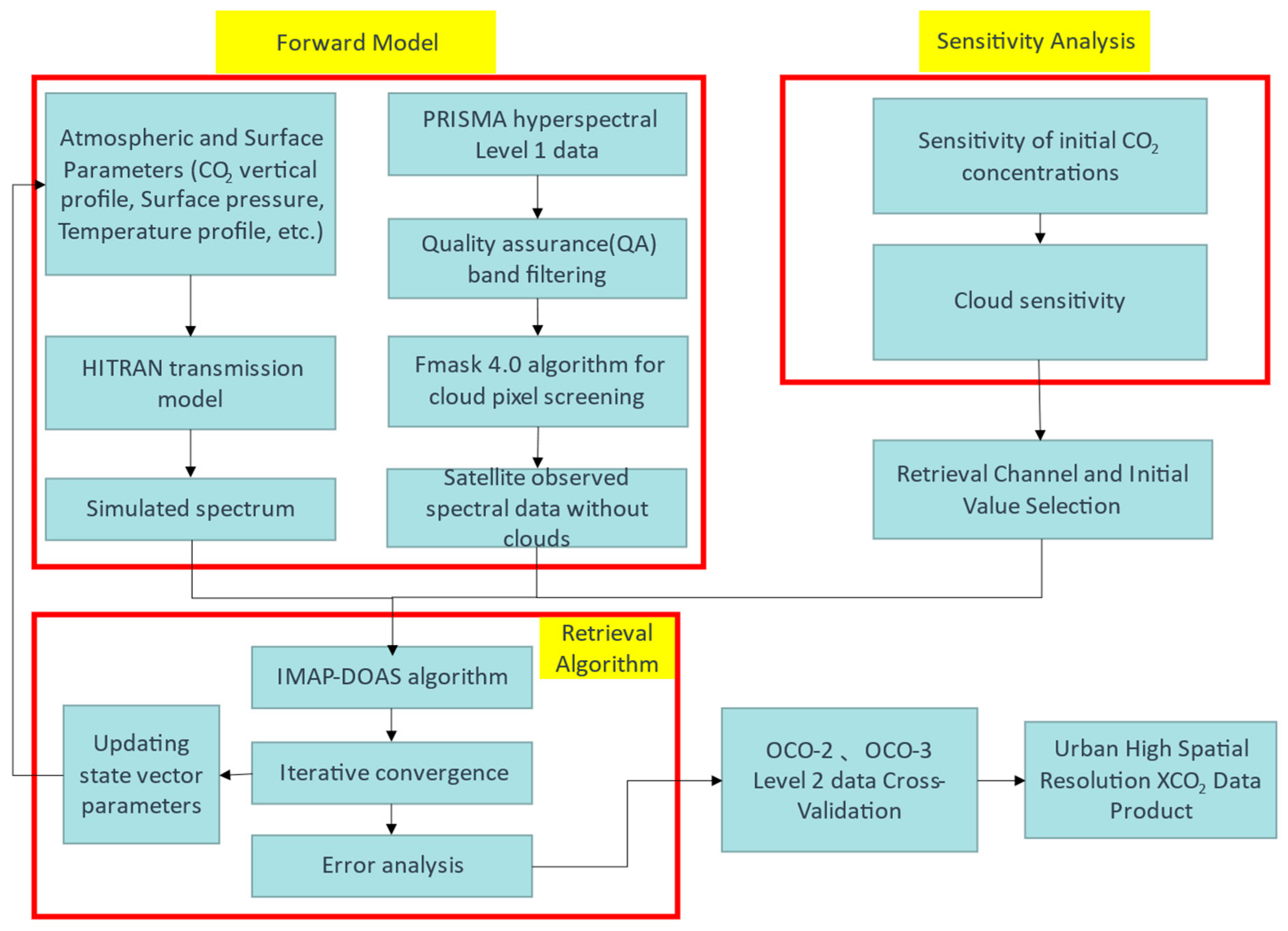
As the reference for the forward model, we utilized the solar spectrum provided by R. Kurucz (http://kurucz.harvard.edu/sun/irradiance2008/, accessed 2 February 2024), which was acquired using the Fourier Transform Spectrometer (FTS) at the Kitt Peak National Observatory. This spectrum covers wavelengths ranging from 1560 nm to 2100 nm, exhibiting an impressive resolution of approximately 0.001 nm [33].

For building the forward model, we selected surface pressure, pressure levels, specific humidity, temperature profiles, and pressure thickness data from the MERRA-2 satellite (https://disc.gsfc.nasa.gov, accessed on 2 February 2024). In this study, we conducted simulations of CO₂, N₂O, H₂O, and dry air concentrations at 72 pressure levels, utilizing MERRA-2 data. Due to the variability of the dry air content throughout the vertical column, it is necessary to consider the impact of this factor on the changes in the concentration of the gas being measured. Since the column is divided into 72 pressure levels, corrections for the gas absorption coefficient at each layer have been made based on actual meteorological data to ensure the accuracy of the gas content in each layer as much as possible. By calculating the average values, we aim to maximize the smoothing of errors caused by variations in gas content. Subsequently, the vertical optical thickness of CO₂, N₂O, and H₂O was determined by employing the HIgh-resolution TRANsmission molecular absorption database (HITRAN, 2016) [34] and applying the classical Voigt spectral line shape.

Furthermore, the vertical column density of dry air was calculated using the dry air profiles. This parameter signifies the overall quantity of dry air within the vertical column. Employing these datasets and models in the forward model allowed us to simulate atmospheric absorption and obtain the vertical column densities of CO₂, N₂O, H₂O, and dry air, which played a crucial role in the CO₂ retrieval process.

3. Methods

3.1. Sensitivity Analysis

In the inversion of urban XCO₂, the crucial aspect lies in accurately simulating the atmospheric radiative transfer forward model. The precise inversion of the atmospheric radiative transfer model is a primary requirement for monitoring urban XCO₂. The forward model simulates the radiation received by the satellite payload after the scattering of solar radiation in the atmosphere and reflection from the Earth’s surface. However, inherent errors in atmospheric parameters contribute to an increasing disparity between simulated spectra and actual observed spectra, impacting the accuracy of urban XCO₂ inversion. Therefore, when constructing the forward model, it is essential to carefully exclude major related parameters such as CO₂ concentration, water vapor, aerosols, and clouds, as these factors can introduce interference and errors in the inversion process. The sensitivity of individual parameters is reflected in the magnitude of their impact on the output results of the forward model. The greater the change in output results with variations in a specific parameter, the higher its sensitivity. Sensitivity can be quantified by the rate of change in gas transmittance. The quantification formula is as follows [35]:

$$N=\frac{T_1-T_0}{T_0}\times 100\%$$

(1)

where $N$ represents the rate of change in gas transmittance, $T_0$ denotes the gas transmittance under the baseline parameters, and $T_1$ represents the gas transmittance after modifying the parameters. Aerosols and clouds in the atmosphere cause light scattering, altering the distribution of photon paths. Therefore, aerosols and clouds are generally considered major error sources in XCO₂ inversion. Different types of cloud layers also exhibit varying abilities to scatter solar radiation, necessitating analysis and discussion of their impacts.

To more accurately monitor urban XCO₂, it is essential to filter and eliminate cloud-related information. Unlike satellites such as GOSAT and TanSat, the PRISMA satellite lacks dedicated cloud and aerosol imaging instruments for precise cloud identification in sync with spectral data. Therefore, we developed the FIMAP-DOAS algorithm to address the challenge of accurate cloud identification and removal of cloud interference in PRISMA satellite data.

3.2. FIMAP-DOAS Algorithm

The Fmask algorithm is based on extracting cloud layers using the cloud’s physical properties and predicting cloud geometry to match potential cloud layers, ultimately generating a cloud mask technology. This algorithm was initially proposed by Zhe Zhu [36] and is designed specifically for Landsat series satellite data. Its core principle can be expressed as

$$NDVI=\frac{B{4}_{(750-900\mathrm{nm})}-B{5}_{(1550-1750\mathrm{nm})}}{B{4}_{(750-900\mathrm{nm})}+B{5}_{(1550-1750\mathrm{nm})}}$$

(2)

$$NDSI=\frac{B{2}_{(525-605\mathrm{nm})}-B{5}_{(1550-1750\mathrm{nm})}}{B{2}_{(525-605\mathrm{nm})}+B{5}_{(1550-1750\mathrm{nm})}}$$

(3)

where $NDVI$ represents the normalized difference vegetation index, $NDSI$ represents the normalized difference snow index, and Bi represents the data for the i-th band of Landsat satellite data. Due to the bright and cold characteristics of clouds, the $NDVI$ and $NDSI$ values for clouds are typically around zero. The Fmask algorithm uses a threshold of 0.8, categorizing data with $NDVI$ and $NDSI$ values below 0.8 as potential cloud layer data.

Simultaneously, utilizing the absolute difference between clouds in the visible light band and background brightness, the whiteness index is proposed, defined as [36]

$$\overline{VIS}=\frac{B{1}_{(450-515\mathrm{nm})}+B{2}_{(525-605\mathrm{nm})}+B{3}_{(630-690\mathrm{nm})}}{3}$$

(4)

$$W\mathrm{hite}ness=\frac{{\displaystyle \sum _{i=1}^3\sqrt{{(Bi-\overline{VIS})}^2}}}{3}$$

(5)

where $\overline{VIS}$ is the average radiation value of the first three bands of Landsat, the Whiteness index is not very useful for Landsat satellite data with only three visible light bands. However, PRISMA, equipped with 66 narrow-band visible light bands, can effectively utilize this index for cloud identification and exclusion. Additionally, further research by Zhe Zhu et al. [37,38] validated the Fmask algorithm for cloud, snow, and haze recognition on Landsat 4–8 and Sentinel satellites. The algorithm has been updated to version 4.0 based on their findings.

For the PRISMA data in this study, given the flat terrain of the Shanghai region without significant mountainous areas, our primary focus is on cloud filtering and removal during the inversion process. Therefore, we have made the following improvements to the algorithm:

$$NDVI=\frac{\overline{B_{42-56}}-\overline{B_{127-147}}}{\overline{B_{42-56}}+\overline{B_{127-147}}}$$

(6)

$$NDSI=\frac{\overline{B_{17-27}}-\overline{B_{127-147}}}{\overline{B_{17-27}}+\overline{B_{127-147}}}$$

(7)

$$W\mathrm{hite}nes{s}_{-}\mathrm{P}=\frac{{\displaystyle \sum _{i=7}^{36}\sqrt{{(Bi-\overline{B})}^2}}}{30}$$

(8)

The spectral range for $NDVI$ is 754.47–902.80 nm, for $NDSI$ is 527.30–609.95 nm, and for $W\mathrm{hite}nes{s}_{-}\mathrm{P}$ is 1554.81–1755.83 nm. We have made corresponding improvements to the parameters mentioned above. Compared to the original Fmask algorithm, the current parameters can better leverage the hyperspectral characteristics of the PRISMA satellite, providing ten times the accuracy compared to Landsat satellites. This enhancement enables more effective identification and differentiation of cloud layers.

The DOAS (Differential Optical Absorption Spectroscopy) algorithm [39] can be described by the following equation:

$$I=I_{0}exp\left(-\sigma \left(v\right)\int C\left(s\right)ds\right)$$

(9)

Here, $I$ indicates the satellite’s actual received radiance in this instance. $I_0$ represents the solar radiation that was utilized as a baseline. $\sigma \left(v\right)$ shows the inverted gas’s cross-sectional absorption in each wavelength. $C\left(s\right)$ is the concentration of the target gas along the radiative transport route.

The FIMAP-DOAS algorithm is an extension of the DOAS algorithm, and its core algorithm has been demonstrated to be effective by Frankenberg [40,41]. This algorithm utilizes the HITRAN radiative transfer model for calculations. The model enables the computation of radiance at each wavelength using the following formula [42]:

$$F^{\mathrm{h}}\left(x\right)=I_0(\lambda )·exp\left(-{\displaystyle {\sum }_{\mathrm{n}=1}^{72}{A}_n·{\tau }_n·x_n}\right)·{\displaystyle \sum }_{k=0}^K{a}_k·{\lambda }^k$$

(10)

Here $F^{\mathrm{h}}\left(x\right)$ represents the forward radiance, $I_0(\lambda )$ is the solar transmittance spectrum. $A_n$ stands for the air mass factor. ${\tau }_n$ is the nth target gas state vector’s reference optical thickness. $x_n$ represents the state vector of the target gas, $a_k$ is a polynomial coefficient, which represents low-frequency features such as surface reflectance.

To calculate the default optical depths, the MERRA-2 meteorological information is queried, as described by Gelaro et al. [43]. The appropriate HITRAN absorption cross-sections are selected based on the calculated optical depths, as described by Kochanov et al. [35]. The simulated spectra are produced between the wavelengths of 1900 and 2100 nm with a spectral precision of 0.02 nm.

The state vector for the target gases encompasses scaling factors for CO₂, H₂O, and N₂O, as well as polynomial coefficients to capture low-frequency features. Moreover, it includes spectral offsets to account for wavelength position uncertainties, following the methodologies introduced by Cusworth et al. [44] and Thorpe et al. [45] for their determination. The observed radiance can be represented as

$$y=F\left(x\right)+\epsilon$$

(11)

The observation error $\epsilon$ is the total of the instrument and forward model errors. To address the mismatch between simulated data and prior information, we employ a Bayesian approach. Since the state equation is nonlinear, iterative methods are required to solve it. The radiation intensity’s Jacobian matrix, $K$, must be determined for each cycle. We obtain the equivalent Jacobian matrix by finding the partial derivative of the state vector x:

$$K=\frac{\partial F}{\partial x}$$

(12)

For such unconstrained problems, obtaining the general solution often requires solving its second-order Hessian matrix. Due to the nonlinear nature of the state vector, this undoubtedly introduces significant computational challenges. Rodgers [46] proposed solving the problem through iterative processes using the least squares method. Subsequent research optimized this approach by employing the Gauss-Newton method to reduce the number of iterations, ensuring convergence of the state vector within a few iterations and reducing computational costs. Therefore, we employ the Gauss-Newton method for iterative optimization to obtain the optimal state vector. The iterative equation is as follows [47]:

$$x_{i+1}=x_{\alpha }+{(K_i^T{S}_i^{-1}{K}_i+S_{\alpha }^{-1})}^{-1}{K}_i^T{S}_i^{-1}\cdot [y-F(x_i)+K_i(x_i-x_{\alpha })]$$

(13)

where $x_{\alpha }$ represents the prior estimate, $x_i$ Indicates the value of x when iterating to the i-th time, $S_i$ denotes the covariance noise matrix, $S_{\alpha }$ represents the covariance error matrix, $F(x_i)$ indicates the forward model’s expected value of $x_i$, and $K_i$ indicates the forward model’s Jacobi matrix.

The complete flowchart of the FIMAP-DOAS algorithm is shown in Figure 2.

3.3. Validation of the Retrieval Results

Due to the different spatial resolutions of PRISMA hyperspectral data (with an XCO₂ single pixel size of 30 × 30 square meters) and OCO-2/OCO-3 satellite L2 data (with an XCO₂ single footprint spatial range of 2.25 × 1.29 square kilometers), a direct comparison between the two datasets is not feasible. Therefore, when selecting validation data from the OCO series satellites, we ensured that the chosen data covered the PRISMA-observed area both temporally and spatially.

The high spatial resolution of the PRISMA satellite results in a larger time resolution, making the PRISMA XCO₂ data relatively sparse along the temporal axis. To address this, we aggregated the XCO₂ data from PRISMA, OCO-2, and OCO-3 satellites on a monthly basis, focusing on regions with matched time and space. By calculating the average XCO₂ value for this region, we performed cross-validation for XCO₂ among the three satellites. Statistical metrics, including root mean square error (RMSE), were computed to quantify the errors. This approach allowed us to assess the accuracy of the inversion results and further explore the precision of the PRISMA satellite in urban XCO₂ inversion monitoring. Detailed explanations of the validation process are provided in Section 4.2.

4. Results and Discussion

4.1. Sensitivity Analysis Results

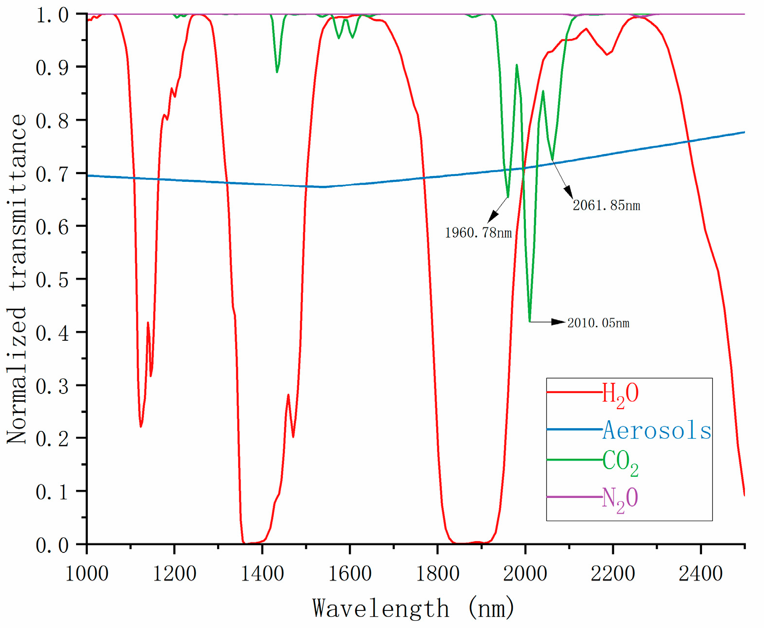
4.1.1. Transmittance Spectrum Analysis

In the forward model development work, we utilized absorption cross-section data from the HITRAN database for sensitivity analysis of inversion-related parameters. Figure 3 displays transmittance spectra in the SWIR (Short-Wave Infrared) region for CO₂, H₂O, N₂O, clouds, and aerosols in the Shanghai region. It reveals significant absorption peaks of CO₂ in the 1900–2100 nm wavelength range. This spectral window can serve as an XCO₂ inversion window. Similarly, the impact of clouds and aerosols on the inversion is significant, requiring a focused analysis.

4.1.2. Sensitivity Analysis of CO₂ Initial Conditions

FIMAP-DOAS requires iterative processing of initial spectral data, and the analysis of CO₂ initial values is crucial.

Table 2. Normalized transmittance sensitivity analysis for initial concentrations of CO₂.

Initial Concentrations of CO2	Average Deviation (%)	Peak Deviation (%)
380 ppm	0	0
390 ppm	−0.3	−0.85
400 ppm	−0.60	−1.67
410 ppm	−0.89	−2.48

illustrates the sensitivity of spectral transmittance to different initial concentrations of CO₂. The four lines in the graph represent the variations in transmittance under four different CO₂ initial values. Using 380 ppm as the baseline, we calculated the normalized transmittance change rates for CO₂ initial concentrations of 390, 400, and 410 ppm. The results indicate that in the spectral range of 1940–2100 nm, as the CO₂ initial concentration increases, the normalized transmittance gradually decreases. Approximately every increase of 10 ppm in CO₂ initial value leads to a 0.3% error in the transmittance spectrum. Therefore, it is essential to set a reasonable initial concentration of CO₂ in the inversion study. In this study, considering the actual conditions in the Shanghai region, we chose 400 ppm as the inversion initial value.

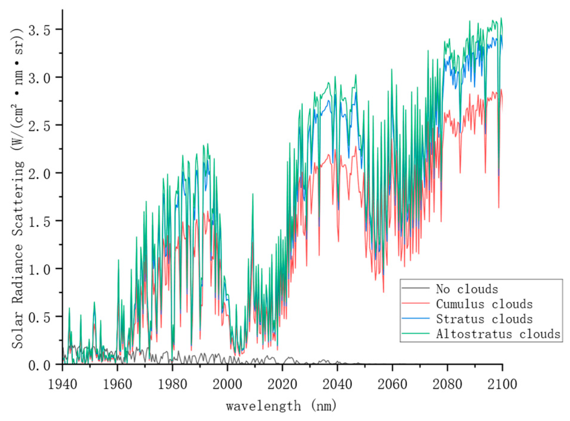
4.1.3. Sensitivity Analysis of Cloud Layer Type

Clouds and aerosols have the capability to scatter solar radiation, thereby influencing the reception of spectral data by satellite instruments. Figure 4 illustrates the scattering ability of different cloud layers for solar radiation. The four lines represent scenarios with no clouds, cumulus clouds, stratus clouds, and altostratus clouds, showcasing their respective abilities to scatter solar radiation. From the graph, it can be observed that in the inversion window of 1940–2100 nm, little to no solar radiation scattering occurs in the absence of clouds. However, in the presence of clouds, significant scattering of solar radiation takes place, introducing substantial errors to XCO₂ inversion. While there are subtle differences in the scattering abilities of cumulus, stratus, and altostratus clouds, the interference in the case of no clouds is substantial and critical. Hence, the FIMAP-DOAS algorithm excels in identifying and removing cloud pixels, effectively avoiding errors introduced by solar radiation scattering from clouds, thereby enhancing the accuracy of the inversion results.

4.2. Spatial and Temporal Variations in XCO₂

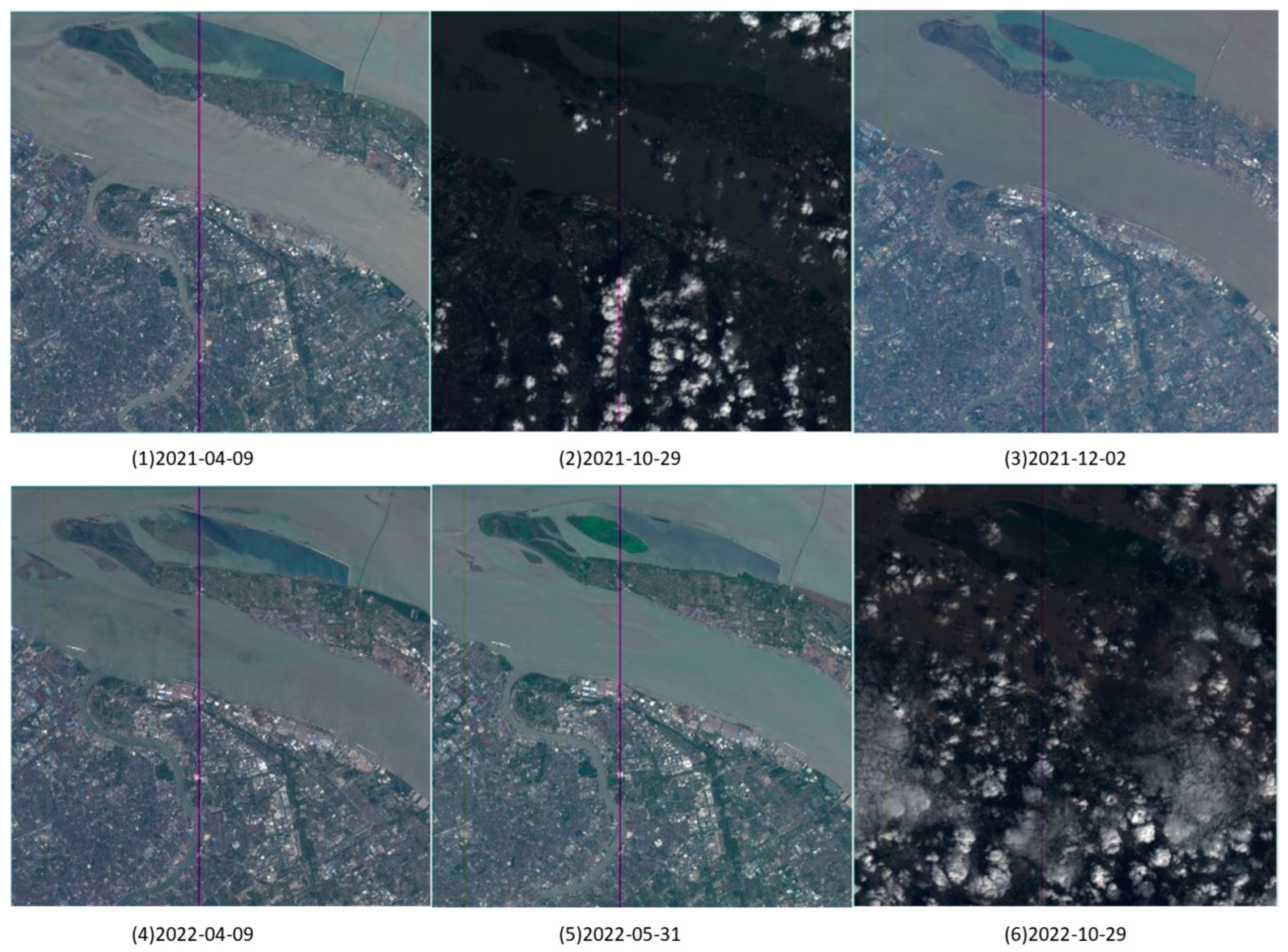
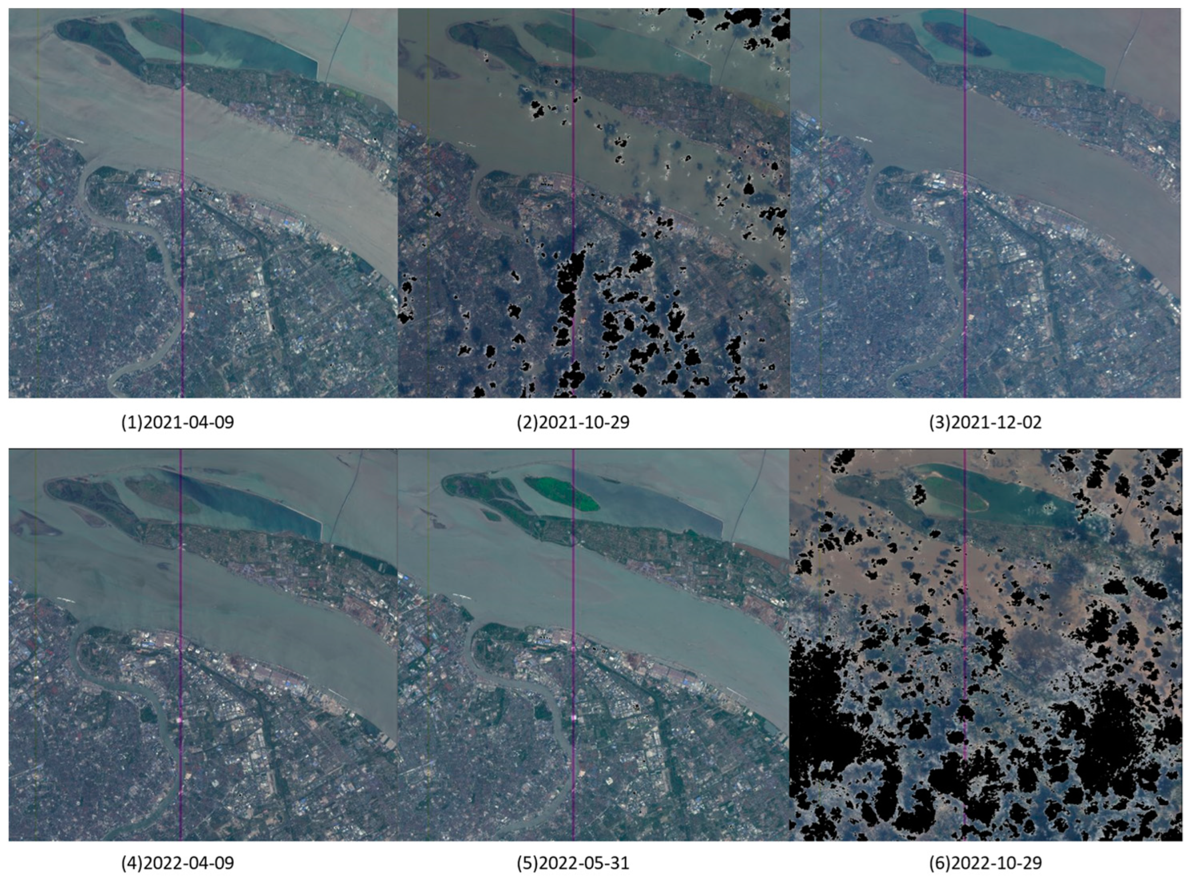
4.2.1. Cloud Removal Results

The previous section has analyzed the interference of cloud layers in the satellite-based XCO₂ inversion; the exclusion of cloudy pixels is essential for the accurate inversion and monitoring of XCO₂ in urban areas. The FIMAP-DOAS algorithm effectively addresses this challenge. After using the FIMAP-DOAS algorithm to identify cloud pixels, all the cloud pixels in the hyperspectral image form a cloud mask. This mask can be directly applied to cover pixels containing clouds in the original hyperspectral image. During the iterative inversion process, these masked pixels are skipped, ensuring a more precise inversion of urban XCO₂ concentrations. Figure 5 illustrates the results of the PRISMA satellite hyperspectral data after processing with the FIMAP-DOAS algorithm. Images (1), (3), (4), and (5) show favorable observation conditions with minimal cloud content, exhibiting little change from the initial image. Images (2) and (6) reveal prominent cloud information, with the black portions indicating cloud pixels identified by the algorithm. These pixels are excluded and no longer participate in the inversion calculation.

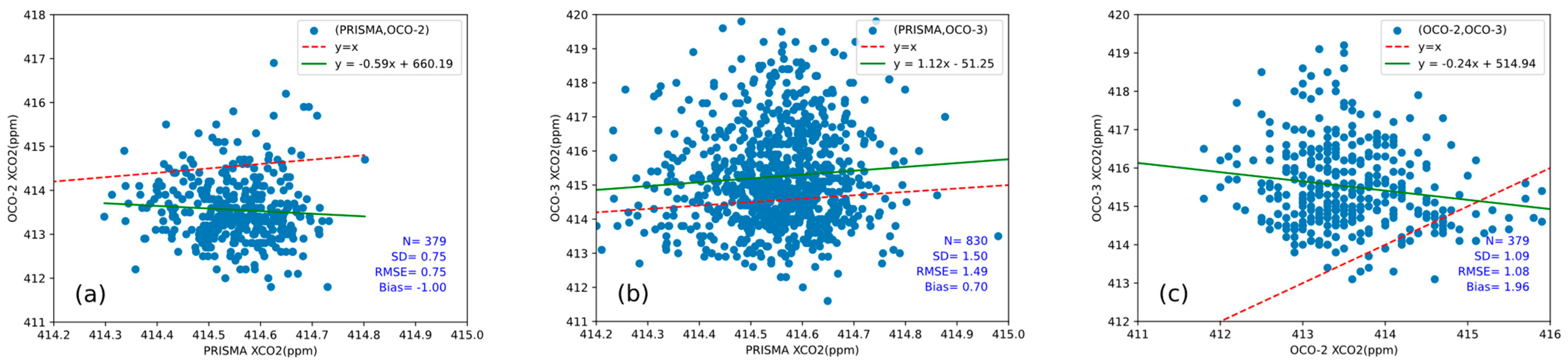
4.2.2. Cross-Validation of PRISMA Using OCO Series Level 2 Product

This study analyzes PRISMA’s XCO₂ inversion using Level 2 XCO₂ data products from OCO-2 and OCO-3 satellites. The time range covers from April 2021 to December 2022. Due to the sparse temporal resolution of PRISMA’s hyperspectral images for the same region, the satellite data results are averaged on a monthly basis for maximum matching verification. Spatial resolution is matched with the OCO-2 satellite as the reference.

Table 3. Monthly average XCO₂ from PRISMA satellite and OCO series satellites.

	Time	2021-04	2021-10	2021-12	2022-04	2022-05	2022-10
Satellite
PRISMA		412.51 ppm	413.12 ppm	414.51 ppm	407.99 ppm	413.75 ppm	414.16 ppm
OCO-2			413.55 ppm	415.67 ppm	409.14 ppm	413.68 ppm	415.51 ppm
OCO-3			414.92 ppm	416.36 ppm	411.21 ppm	414.44 ppm	416.63 ppm

displays the XCO₂ for PRISMA, OCO-2, and OCO-3 satellites in the region, averaged monthly. Due to variations in the operation of each satellite and limited spatiotemporal co-location, some blank situations exist in the XCO₂ data of the satellites in the table. However, the overall distribution shows lower XCO₂ in spring and summer and higher XCO2 in autumn and winter, which is consistent with the spatiotemporal distribution of XCO₂. The absolute error between PRISMA’s inverted XCO₂ and OCO-2, OCO-3 XCO₂ is within 3 ppm, meeting the requirement of inversion error below 1% for satellites.

To assess the reliability of the PRISMA satellite retrieval and monitoring of urban XCO₂, we conducted quantitative cross-validation by comparing PRISMA inversion results with Level 2 data products from OCO-2 and OCO-3 satellites. Before the quantitative analysis, we divided the three products into numerous small windows of 2.25 km × 1.29 km based on the spatial resolution of OCO-2. Subsequently, we selected grids with the same longitude and latitude for the same month, resulting in 379 valid matching points for OCO-2 and 830 for OCO-3. We performed a linear analysis of XCO₂, and Figure 6a–c show scatter plots of XCO₂ correlations between pairs of the three satellites. Figure 6c serves as a reference comparison between XCO₂ from OCO-2 and OCO-3. From the images, it is evident that the linear correlation between PRISMA satellite XCO₂ products and OCO-3 XCO₂ products is better, with the fitting line closer to the line-to-line connection. Specifically, the bias error of PRISMA satellite inversion XCO₂ compared to OCO-2 satellite data is −1.00 ppm, while compared to OCO-3 satellite data, the bias error is 0.70 ppm. The former has a standard deviation (SD) and root mean square error (RMSE) of 0.75 ppm and 0.75 ppm, respectively, while the latter has an SD and RMSE of 1.50 ppm and 1.49 ppm, respectively.

4.3. Discussion of Strengths and Limitations

The main objective of this study is to achieve the inversion and monitoring of XCO₂ in small-scale urban areas. The proposed FIMAP-DOAS algorithm addresses the issue of interference from cloud pixels in PRISMA satellite hyperspectral images, making optimal use of PRISMA hyperspectral satellite data. The algorithm successfully establishes a comprehensive system for the inversion and monitoring of XCO₂ in urban areas. It accurately inverts XCO₂ and enables long-term time series monitoring of XCO₂ in the same region. Additionally, the high spatial resolution of the PRISMA satellite provides finer inversion data, serving as complementary support to traditional carbon satellite data. This work provides a comprehensive inversion system that offers solid data support for the inversion and monitoring of XCO₂ in urban areas with high spatial resolution. The inversion algorithm enables rapid assessment of a region for high-carbon-emission activities by analyzing XCO₂ concentrations. For instance, the algorithm can identify and conduct long-term monitoring of XCO₂ in high-carbon-emission areas, such as power plants and steel factories. Additionally, to monitor XCO₂ in other urban areas, one simply needs to replace the spectral and meteorological data with those corresponding to the city of interest to achieve XCO₂ inversion and monitoring for that city.

This study has certain limitations. The high spatial resolution of the PRISMA satellite results in a revisit period of 29 days, leading to a relatively low amount of effective data with discontinuous temporal coverage. This poses challenges in the cross-validation process, as obtaining data that simultaneously meets latitude, longitude, and time requirements is challenging. The use of monthly averaged XCO₂ for validation aims to maximize the matching of effective samples. The limitations imposed by the availability of PRISMA satellite data also restrict our choice of monitoring areas. To ensure continuous XCO₂ inversion and monitoring in the same location and to facilitate a better comparison and validation of XCO₂ inversion accuracy, we were compelled to select the area depicted in Figure 1. It is noteworthy, however, that Shanghai is a port city, and the selected area includes a significant international port. In future research, we can focus on monitoring CO₂ emissions from this port. This approach could provide substantial supporting data for various port cities to reduce carbon emissions. Moreover, compared to the OCO series of satellites, the average spectral resolution of PRISMA satellite data may appear coarser. Given that our research goal is to achieve high spatial resolution XCO₂ inversion and monitoring in urban areas, the coarseness of the data’s spectral resolution is inevitable. In the future, we can opt for satellite data that simultaneously consider both spatial and spectral resolution for further optimization and enhancement.

In terms of algorithm structure, FIMAP-DOAS divides the atmosphere into 72 layers for XCO₂ inversion, resulting in concentrated inversion results with fluctuations not exceeding 1 ppm. This also makes the algorithm more sensitive to noise in the L2 data of OCO series satellites during linear analysis. Romaniello et al. [48] proposed a CIBR interpolation algorithm for PRISMA data, combining XCO₂ with surface reflectance to mitigate the influence of CO₂ and H₂O in the inversion range. This results in a smoother algorithm structure, enhanced noise resistance, and higher stability.

Future advancements in algorithm structure are expected to improve overall noise resistance. As time progresses, the PRISMA satellite will provide more hyperspectral data for new algorithm research and validation. In future studies, our team will consider using devices such as drones for ground monitoring and validation, aiming to enhance the accuracy of urban XCO₂ monitoring and inversion. At the same time, we will also pay closer attention to the impact of anthropogenic emissions on the errors and interference in urban area XCO₂ inversion, with the aim of further enhancing the specificity and accuracy of the inversion monitoring system.

5. Conclusions and Outlook

This work successfully established a high spatial resolution satellite monitoring system for urban XCO₂, demonstrating the application of the FIMAP-DOAS algorithm to extract high-resolution (30 m) XCO₂ from PRISMA satellite data in the Shanghai area. The retrieved XCO₂ values exhibited consistent seasonal variations in line with expected CO₂ dynamics. Validation against OCO-2 and OCO-3 Level 2 data showed a bias of −1.00 ppm and RMSE of 0.75 ppm for the former and a bias of 0.70 ppm and RMSE of 1.49 ppm for the latter, meeting the accuracy requirements for satellite XCO₂ inversion. These results confirm the reliability and consistency of PRISMA satellite inversion with actual measurements.

The significance of this study is noteworthy. High spatial resolution XCO₂ inversion enables precise monitoring and analysis of carbon sources in the Shanghai region. This capability supports long-term tracking and analysis, facilitating effective carbon-emission regulation and the formulation of relevant policies by government and regulatory agencies. Furthermore, the application of PRISMA satellite data retrieval for XCO₂ has significant potential. Its cross-validation potential with upcoming high-resolution carbon satellites (such as DQ-1, DQ-2, and Carbon Mapper) further enhances the credibility and accuracy of carbon monitoring.

Future research will focus on optimizing the FIMAP-DOAS algorithm by incorporating additional inversion parameters from satellite observations, surface characteristics, and atmospheric parameters. This optimization will enhance the accuracy and temporal resolution of XCO₂ monitoring, enabling a more detailed and comprehensive assessment of carbon dynamics and contributing to the advancement of carbon monitoring capabilities.

References

1. Huang, T.Y.; Ding, L.P.; Yu, Y.Q.; Huang, L.; Yang, L.Y. From AR5 to AR6: Exploring research advancement in climate change based on scientific evidence from IPCC WGI reports. Scientometrics 2023, 128, 5227–5245. [Google Scholar] [CrossRef]
2. McKay, D.I.A.; Staal, A.; Abrams, J.F.; Winkelmann, R.; Sakschewski, B.; Loriani, S.; Fetzer, I.; Cornell, S.E.; Rockstrom, J.; Lenton, T.M. Exceeding 1.5 °C global warming could trigger multiple climate tipping points. Science 2022, 377, 1171. [Google Scholar] [CrossRef]
3. Rogelj, J.; den Elzen, M.; Höhne, N.; Fransen, T.; Fekete, H.; Winkler, H.; Chaeffer, R.S.; Ha, F.; Riahi, K.; Meinshausen, M. Paris Agreement climate proposals need a boost to keep warming well below 2 °C. Nature 2016, 534, 631–639. [Google Scholar] [CrossRef]
4. Zhao, X.; Ma, X.W.; Chen, B.Y.; Shang, Y.P.; Song, M.L. Challenges toward carbon neutrality in China: Strategies and countermeasures. Resour. Conserv. Recycl. 2022, 176, 9. [Google Scholar] [CrossRef]
5. He, C.P.; Ji, M.R.; Grieneisen, M.L.; Zhan, Y. A review of datasets and methods for deriving spatiotemporal distributions of atmospheric CO2. J. Environ. Manag. 2022, 322, 10. [Google Scholar] [CrossRef] [PubMed]
6. Butz, A.; Guerlet, S.; Hasekamp, O.; Schepers, D.; Galli, A.; Aben, I.; Frankenberg, C.; Hartmann, J.M.; Tran, H.; Kuze, A.; et al. Toward accurate CO2 and CH4 observations from GOSAT. Geophys. Res. Lett. 2011, 38, 6. [Google Scholar] [CrossRef]
7. Imasu, R.; Matsunaga, T.; Nakajima, M.; Yoshida, Y.; Shiomi, K.; Morino, I.; Saitoh, N.; Niwa, Y.; Someya, Y.; Oishi, Y.; et al. Greenhouse gases Observing SATellite 2 (GOSAT-2): Mission overview. Prog. Earth Planet. Sci. 2023, 10, 35. [Google Scholar] [CrossRef]
8. Peiro, H.; Crowell, S.; Schuh, A.; Baker, D.F.; O’Dell, C.; Jacobson, A.R.; Chevallier, F.; Liu, J.J.; Eldering, A.; Crisp, D.; et al. Four years of global carbon cycle observed from the orbiting carbon observatory 2 (OCO-2) version 9 and in situ data and comparison to OCO-2 version 7. Atmos. Chem. Phys. 2022, 22, 1097–1130. [Google Scholar] [CrossRef]
9. Eldering, A.; Taylor, T.E.; O’Dell, C.W.; Pavlick, R. The OCO-3 mission: Measurement objectives and expected performance based on 1 year of simulated data. Atmos. Meas. Tech. 2019, 12, 2341–2370. [Google Scholar] [CrossRef]
10. Liu, Y.; Wang, J.; Yao, L.; Chen, X.; Cai, Z.; Yang, D.; Yin, Z.; Gu, S.; Tian, L.; Lu, N.; et al. TanSat mission achievements: From scientific driving to preliminary observations. Chin. J. Space Sci. 2018, 38, 627–639. [Google Scholar] [CrossRef]
11. Saeki, T.; Saito, R.; Belikov, D.; Maksyutov, S. Global high-resolution simulations of CO2 and CH4 using a NIES transport model to produce a priori concentrations for use in satellite data retrievals. Geosci. Model Dev. 2013, 6, 81–100. [Google Scholar] [CrossRef]
12. O’Dell, C.W.; Connor, B.; Bösch, H.; O’Brien, D.; Frankenberg, C.; Castano, R.; Christi, M.; Crisp, D.; Eldering, A.; Fisher, B.; et al. The ACOS CO2 retrieval algorithm—Part 1: Description and validation against synthetic observations. Atmos. Meas. Tech. 2012, 5, 99–121. [Google Scholar] [CrossRef]
13. Taylor, T.E.; O’Dell, C.W.; Crisp, D.; Kuze, A.; Lindqvist, H.; Wennberg, P.O.; Chatterjee, A.; Gunson, M.; Eldering, A.; Fisher, B.; et al. An 11-year record of XCO2 estimates derived from GOSAT measurements using the NASA ACOS version 9 retrieval algorithm. Earth Syst. Sci. Data 2022, 14, 325–360. [Google Scholar] [CrossRef]
14. Wu, L.H.; Hasekamp, O.; Hu, H.L.; Landgraf, J.; Butz, A.; aan de Brugh, J.; Aben, I.; Pollard, D.F.; Griffith, D.W.T.; Feist, D.G.; et al. Carbon dioxide retrieval from OCO-2 satellite observations using the RemoTeC algorithm and validation with TCCON measurements. Atmos. Meas. Tech. 2018, 11, 3111–3130. [Google Scholar] [CrossRef]
15. Yang, D.X.; Zhang, H.F.; Liu, Y.; Chen, B.Z.; Cai, Z.N.; Lü, D.R. Monitoring carbon dioxide from space: Retrieval algorithm and flux inversion based on GOSAT data and using CarbonTracker-China. Adv. Atmos. Sci. 2017, 34, 965–976. [Google Scholar] [CrossRef]
16. Broquet, G.; Bréon, F.M.; Renault, E.; Buchwitz, M.; Reuter, M.; Bovensmann, H.; Chevallier, F.; Wu, L.; Ciais, P. The potential of satellite spectro-imagery for monitoring CO2 emissions from large cities. Atmos. Meas. Tech. 2018, 11, 681–708. [Google Scholar] [CrossRef]
17. Lauvaux, T.; Miles, N.L.; Richardson, S.J.; Deng, A.J.; Stauffer, D.R.; Davis, K.J.; Jacobson, G.; Rella, C.; Calonder, G.P.; DeCola, P.L. Urban Emissions of CO2 from Davos, Switzerland: The First real-time monitoring system using an atmospheric inversion technique. J. Appl. Meteorol. Climatol. 2013, 52, 2654–2668. [Google Scholar] [CrossRef]
18. Xiang, R.; Yang, H.; Yan, Z.J.; Taha, A.M.M.; Xu, X.; Wu, T. Super-resolution reconstruction of GOSAT CO2 products using bicubic interpolation. Geocarto Int. 2022, 37, 15187–15211. [Google Scholar] [CrossRef]
19. Roten, D.; Wu, D.E.; Fasoli, B.; Oda, T.; Lin, J.C. An interpolation method to reduce the computational time in the stochastic lagrangian particle dispersion modeling of spatially dense XCO2 retrievals. Earth Space Sci. 2021, 8, 28. [Google Scholar] [CrossRef] [PubMed]
20. Nguyen, H.; Cressie, N.; Braverman, A. Multivariate spatial data fusion for very large remote sensing datasets. Remote Sens. 2017, 9, 142. [Google Scholar] [CrossRef]
21. He, S.C.; Yuan, Y.B.; Wang, Z.H.; Luo, L.; Zhang, Z.L.; Dong, H.; Zhang, C.F. Machine Learning Model-Based Estimation of XCO2 with High Spatiotemporal Resolution in China. Atmosphere 2023, 14, 436. [Google Scholar] [CrossRef]
22. Pignatti, S.; Palombo, A.; Pascucci, S.; Romano, F.; Santini, F.; Simoniello, T.; Amato, U.; Cuomo, V.; Acito, N.; Diani, M.; et al. The PRISMA hyperspectral mission: Science activities and opportunities for agriculture and land monitoring. In Proceedings of the IEEE International Geoscience and Remote Sensing Symposium (IGARSS), Melbourne, Australia, 21–26 July 2013; pp. 4558–4561. [Google Scholar]
23. Acito, N.; Diani, M.; Alibani, M.; Corsini, G. Matched filter based on the radiative transfer model for CO2 estimation from PRISMA hyperspectral data. IEEE Trans. Geosci. Remote Sens. 2023, 61, 13. [Google Scholar] [CrossRef]
24. Kai, Q.; Qin, H.; Kang, H.S.; Wei, H.; Fan, L.; Jason, C. Progress and prospect of satellite remote sensing research applied to methane emissions from the coal industry. Acta Opt. Sin. 2023, 43, 13. [Google Scholar] [CrossRef]
25. Crisp, D.; Pollock, H.R.; Rosenberg, R.; Chapsky, L.; Lee, R.A.M.; Oyafuso, F.A.; Frankenberg, C.; O’Dell, C.W.; Bruegge, C.J.; Doran, G.B.; et al. The on-orbit performance of the Orbiting Carbon Observatory-2 (OCO-2) instrument and its radiometrically calibrated products. Atmos. Meas. Tech. 2017, 10, 59–81. [Google Scholar] [CrossRef]
26. Romero-Lankao, P.; Gurney, K.R.; Seto, K.C.; Chester, M.; Duren, R.M.; Hughes, S.; Hutyra, L.R.; Marcotullio, P.; Baker, L.; Grimm, N.B.; et al. A critical knowledge pathway to low-carbon, sustainable futures: Integrated understanding of urbanization, urban areas, and carbon. Earth Future 2014, 2, 515–532. [Google Scholar] [CrossRef]
27. He, J.Q.; Wang, S.J.; Liu, Y.Y.; Ma, H.T.; Liu, Q.Q. Examining the relationship between urbanization and the eco-environment using a coupling analysis: Case study of Shanghai, China. Ecol. Indic. 2017, 77, 185–193. [Google Scholar] [CrossRef]
28. Wang, S.J.; Liu, X.P.; Zhou, C.S.; Hu, J.C.; Ou, J.P. Examining the impacts of socioeconomic factors, urban form, and transportation networks on CO2 emissions in China’s megacities. Appl. Energy 2017, 185, 189–200. [Google Scholar] [CrossRef]
29. Feldman, A.F.; Zhang, Z.; Yoshida, Y.; Chatterjee, A.; Poulter, B. Using Orbiting Carbon Observatory-2 (OCO-2) column CO2 retrievals to rapidly detect and estimate biospheric surface carbon flux anomalies. Atmos. Chem. Phys. 2023, 23, 1545–1563. [Google Scholar] [CrossRef]
30. Taylor, T.E.; O’Dell, C.W.; Baker, D.; Bruegge, C.; Chang, A.; Chapsky, L.; Chatterjee, A.; Cheng, C.; Chevallier, F.; Crisp, D.; et al. Evaluating the consistency between OCO-2 and OCO-3 XCO2 estimates derived from the NASA ACOS version 10 retrieval algorithm. Atmos. Meas. Tech. 2023, 16, 3173–3209. [Google Scholar] [CrossRef]
31. Wunch, D.; Wennberg, P.O.; Osterman, G.; Fisher, B.; Naylor, B.; Roehl, C.M.; O’Dell, C.; Mandrake, L.; Viatte, C.; Kiel, M.; et al. Comparisons of the Orbiting Carbon Observatory-2 (OCO-2) XCO2 measurements with TCCON. Atmos. Meas. Tech. 2017, 10, 2209–2238. [Google Scholar] [CrossRef]
32. Kiel, M.; Eldering, A.; Roten, D.D.; Lin, J.C.; Feng, S.; Lei, R.X.; Lauvaux, T.; Oda, T.; Roehl, C.M.; Blavier, J.F.; et al. Urban-focused satellite CO2 observations from the Orbiting Carbon Observatory-3: A first look at the Los Angeles megacity. Remote Sens. Environ. 2021, 258, 17. [Google Scholar] [CrossRef]
33. Kurucz, R.L. High Resolution Irradiance Spectrum from 300 to 1000 nm. arXiv 2006, arXiv:astro-ph/0605029. [Google Scholar]
34. Kochanov, R.V.; Gordon, I.E.; Rothman, L.S.; Wcislo, P.; Hill, C.; Wilzewski, J.S. HITRAN Application Programming Interface (HAPI): A comprehensive approach to working with spectroscopic data. J. Quant. Spectrosc. Radiat. Transfer 2016, 177, 15–30. [Google Scholar] [CrossRef]
35. Zhao, L.; Chen, S.; Xue, Y.; Cui, T. Study of atmospheric carbon dioxide retrieval method based on normalized sensitivity. Remote Sens. 2022, 14, 1106–1125. [Google Scholar] [CrossRef]
36. Zhu, Z.; Woodcock, C.E. Object-based cloud and cloud shadow detection in Landsat imagery. Remote Sens. Environ. 2012, 118, 83–94. [Google Scholar] [CrossRef]
37. Zhu, Z.; Wang, S.; Woodcock, C.E. Improvement and expansion of the Fmask algorithm: Cloud, cloud shadow, and snow detection for Landsats 4–7, 8, and Sentinel 2 images. Remote Sens. Environ. 2015, 159, 269–277. [Google Scholar] [CrossRef]
38. Qiu, S.; He, B.; Zhu, Z.; Liao, Z.; Quan, X. Improving Fmask cloud and cloud shadow detection in mountainous area for Landsats 4–8 images. Remote Sens. Environ. 2017, 199, 107–119. [Google Scholar] [CrossRef]
39. Wang, S.; Zhou, B. Progress in aerosol measurements based on differential optical absorption spectroscopy method. J. Atmos. Environ. Opt. 2015, 10, 139–148. [Google Scholar]
40. Frankenberg, C.; Platt, U.; Wagner, T. Iterative maximum a posteriori (IMAP)-DOAS for retrieval of strongly absorbing trace gases: Model studies for CH4 and CO2 retrieval from near infrared spectra of SCIAMACHY onboard ENVISAT. Atmos. Chem. Phys. 2005, 5, 9–22. [Google Scholar] [CrossRef]
41. Frankenberg, C.; Thorpe, A.K.; Thompson, D.R.; Hulley, G.; Kort, E.A.; Vance, N.; Borchardt, J.; Krings, T.; Gerilowski, K.; Sweeney, C.; et al. Airborne methane remote measurements reveal heavy-tail flux distribution in Four Corners region. Proc. Natl. Acad. Sci. USA 2016, 113, 9734–9739. [Google Scholar] [CrossRef]
42. Cusworth, D.H.; Duren, R.M.; Thorpe, A.K.; Eastwood, M.L.; Green, R.O.; Dennison, P.E.; Frankenberg, C.; Heckler, J.W.; Asner, G.P.; Miller, C.E. Quantifying global power plant carbon dioxide emissions with imaging spectroscopy. AGU Adv. 2021, 2, e2020AV000350. [Google Scholar] [CrossRef]
43. Gelaro, R.; McCarty, W.; Suarez, M.J.; Todling, R.; Molod, A.; Takacs, L.; Randles, C.A.; Darmenov, A.; Bosilovich, M.G.; Reichle, R.; et al. The Modern-Era retrospective analysis for research and applications, version 2 (MERRA-2). J. Clim. 2017, 30, 5419–5454. [Google Scholar] [CrossRef]
44. Cusworth, D.H.; Jacob, D.J.; Varon, D.J.; Miller, C.C.; Liu, X.; Chance, K.; Thorpe, A.K.; Duren, R.M.; Miller, C.E.; Thompson, D.R.; et al. Potential of next-generation imaging spectrometers to detect and quantify methane point sources from space. Atmos. Meas. Tech. 2019, 12, 5655–5668. [Google Scholar] [CrossRef]
45. Thorpe, A.K.; Frankenberg, C.; Thompson, D.R.; Duren, R.M.; Aubrey, A.D.; Bue, B.D.; Green, R.O.; Gerilowski, K.; Krings, T.; Borchardt, J.; et al. Airborne DOAS retrievals of methane, carbon dioxide, and water vapor concentrations at high spatial resolution: Application to AVIRIS-NG. Atmos. Meas. Tech. 2017, 10, 3833–3850. [Google Scholar] [CrossRef]
46. Rodgers, C.D. Retrieval of atmospheric temperature and composition from remote measurements of thermal radiation. Rev. Geophys. 1976, 14, 609–624. [Google Scholar] [CrossRef]
47. Rodgers, C.D. Inverse Methods for Atmospheric Sounding: Theory and Practice; World Scientific: Singapore, 2000; Volume 2. [Google Scholar]
48. Romaniello, V.; Spinetti, C.; Silvestri, M.; Buongiorno, M.F. A methodology for CO2 retrieval applied to hyperspectral PRISMA data. Remote Sens. 2021, 13, 4502. [Google Scholar] [CrossRef]
Figure 1. PRecursore IperSpettrale della Missione Applicativa (PRISMA) satellite hyperspectral images of Baoshan District in Shanghai. Each subfigure in the figure represents a hyperspectral remote sensing image of the same location in Baoshan District, Shanghai, at different time points. Each image covers an area of 30 km × 30 km, and each pixel represents a ground area of 30 m × 30 m.
Atmosphere 15 00246 g001
Figure 2. The full flowchart of the FIMAP-DOAS retrieval algorithm.
Atmosphere 15 00246 g002
Figure 3. Transmittance spectral plots of crucial inversion parameters.
Atmosphere 15 00246 g003
Figure 4. Spectral lines of solar radiation scattering for different cloud types.
Atmosphere 15 00246 g004
Figure 5. PRISMA hyperspectral image processed with the FIMAP-DOAS algorithm. Each subfigure represents a remote sensing image after applying the Fmask cloud removal algorithm. In subfigures (2) and (6), the black areas indicate the cloud pixels identified by the algorithm. These cloud pixels are excluded from the inversion process. Each image covers an area of 30 km × 30 km, and each pixel represents a ground area of 30 m × 30 m.
Atmosphere 15 00246 g005
Figure 6. Scatter plot comparing PRISMA retrieval with OCO-2 and OCO-3 products, Subfigure (a) represents the comparison results between the PRISMA satellite and the OCO-2 satellite. Subfigure (b) represents the comparison results between the PRISMA satellite and the OCO-3 satellite. Subfigure (c) serves as the control group, representing the comparison results between the OCO-2 and OCO-3 satellites. Where N represents sample size, SD represents standard deviation, RMSE represents root mean square error, Bias represents bias error, the red line represents the one-to-one line, and the green line represents the linear regression fit of the data.
Atmosphere 15 00246 g006