Black Carbon along a Highway and in a Residential Neighborhood during Rush-Hour Traffic in a Cold Climate

Abstract

Short-term exposure to ultra-fine Black Carbon (BC) particles produced during incomplete fuel combustion of wood and fossil fuel has been linked to respiratory and cardiovascular diseases, hospitalizations and premature deaths. The goal of this research was to assess traffic-related BC in a cold climate along an urban highway and 300 m into an adjacent residential neighborhood. BC was measured with an aethalometer (MA350, Aethlabs) along the main traffic artery in geothermally heated Reykjavík, the capital of Iceland (64.135° N–21.895° W, 230,000 inhabitants). Stationary monitoring confirmed that traffic was the dominant source of roadside BC in winter, averaging 1.0 ± 1.1 µg/m³ (0.6 and 1.1 µg/m³ median and interquartile range; 28,000 vehicles/day). Inter-day variations in BC were primarily correlated to the atmospheric lapse rate and wind speed, both during stationary and mobile campaigns. During winter stills, BC levels surpassed 10 µg/m³ at intersections and built up to 5 µg/m³ during the afternoon in the residential neighborhood (adjacent to the highway with 43,000 vehicles/day). The BC penetrated deeply into the neighborhood, where the lowest concentration was 1.8 µg/m³ within 300 m. BC concentration was highly correlated to nitrogen dioxide (r > 0.8) monitored at the local Urban Traffic Monitoring site.

1. Introduction

Urban air quality is a growing public and environmental health concern as more and more people migrate to cities. In Europe, 90% of the urban population was exposed to harmful levels of fine particulate matter (PM_2.5) and nitrogen dioxide (NO₂) [1], attributing to 417,000 and 55,000 premature deaths in 2018, respectively [2]. The chemical composition and toxicity of fine particles vary by source, with diesel engine exhaust particles being the most toxic, followed by gasoline engine exhaust particles, biomass burning particles and road dust [3]. Black Carbon (BC, soot) is a component of solid particles generated during incomplete fuel combustion. Freshly emitted BC consists of ultra-fine particles in the 10–100 nm diameter range [4] that can penetrate deep into the lungs and pass through membranes into the blood stream. Short-term exposure to BC has been connected to an increased number of adult cardiovascular and pediatric respiratory hospitalizations [5] and mortality [6], even when the 24 h ambient air quality standard for PM_2.5 of 35 µm/m³ was not exceeded [7]. Daily variations in BC concentrations may better indicate the short-term health effects of harmful combustion-generated particulate substances than PM [4]. An official air quality guideline has yet to be defined for BC [8].

The road transport sector was the second largest contributor of BC in Europe in 2018, responsible for 26% of the total BC emissions, and lagging the commercial, institutional and household fuel combustion sectors by 11% [2]. Many factors affect traffic-related BC levels in urban areas. First and foremost is traffic intensity, in particular the number of diesel-powered and heavy-duty vehicles [9,10]. Pollution dilution is, in turn, affected by atmospheric conditions, such as solar radiation and wind speed, and their interaction with buildings and moving vehicles [11,12]. Urban BC sources and mixing mechanisms thus vary spatially [13], which is not well captured by stationary air quality measurements [14,15]. Mobile monitoring more accurately captures public exposure to urban air pollution, providing a foundation for more effective mitigation measures [16]. Mobile campaigns have stressed that both adults and children may receive ~20% of their BC dose while commuting, even though it only represents 6% of daily activities [17,18].

The cold climate is particularly prone to developing high traffic-related BC and PM pollution since less efficient fuel combustion during frost emits more exhaust gases. Moreover, very stable atmospheric conditions develop during frost stills, trapping pollution near the ground [19,20,21]. However, BC originating from fossil fuel combustion is often masked by increased residential and commercial wood and coal-burning practices in winter [22]. From this perspective, Iceland is an interesting country to study traffic-related BC in a cold climate because the road transport sector is by far the largest contributor to BC, comprising 45% of the national BC emissions [23]. Household heating, in turn, is for the most part an irrelevant source of BC because of the prevalent use of district heating with geothermal water. Manufacturing and construction activities constitute 30% of BC, while commercial fishing accounts for 10% of national BC emissions [23]. BC was not detected near the Old Harbor in a scoping study in the capital city of Reykjavík in fall 2017 [24].

Reykjavík is the world’s northernmost capital (64.135° N, −21.895° W). The city center lies at the tip of a peninsula (Figure 1, insert), which contributes to traffic being consolidated on a few major highway arteries, with more heavy traffic than would be expected for an urban population of 230,000. The growing car fleet, including a greater share of diesel-fueled cars [25], has contributed to regular exceedances of the 24 h PM₁₀ concentration limit value of 50 µg/m³ in winter and spring [26]. In 2017 and 2018, the 24 h NO₂ concentration limit value of 75 µg/m³ was exceeded on 33 days, as compared to only 2 days in the previous 13 years [27,28]. Source apportionment studies have hinted that BC may be an increasing source of PM₁₀ [29]. On the other hand, the capital receives a fresh supply of air from the open ocean. On an annual basis, the city air can be considered very clean, with NO₂ and PM₁₀ concentrations ranging between 16 and 27 µg/m³ [28].

The overarching objective of this research was to assess the traffic-related BC footprint near an urban highway in a cold climate when the air temperature ranges from −6 °C to +10 °C. The study focused particularly on resolving the upper range of BC concentrations that the public could be exposed to during rush-hour traffic along or adjacent to an urban highway with heterogeneous surroundings. Moreover, an effort was made to understand when, where and why high traffic-related BC develops and how far it penetrates into a residential neighborhood. To that end, the most central traffic artery in Reykjavík City was monitored both via stationary and mobile campaigns, the latter targeting days with high traffic-related PM₁₀ and/or NO₂ pollution in winter and spring.

2. Materials and Methods

2.1. Study Site

The Miklabraut (MIK)–Hringbraut (HRI) Highway was chosen as a study site to resolve high traffic-related BC concentrations in a heterogeneous urban environment for several reasons (Figure 1): (1) its dominant traffic volume in Reykjavík City; (2) its proximity to residential, recreational, commercial and educational areas frequented by all citizens, including groups that are sensitive to air pollution such as children and the elderly; (3) the availability of official weather and air quality data; and (4) its diverse landscape that can affect pollution levels. The highway is framed by two-to-four-story residential buildings and/or tall trees, with four lanes near the city center separated by a vegetated median strip (Figure 2a), widening to four lanes in each direction away from the center (Figure 2b,c).

2.2. BC Monitoring Campaigns Design

Black carbon was monitored with a new, factory-calibrated MA350 aethalometer from Aethlabs (San Francisco, CA, USA). The instrument is a 5-wavelength (880 nm [IR], 625 nm [Red], 528 nm [Green], 470 nm [Blue], and 375 nm [UV]), dual-spot aethalometer. The instrument detection limit is 30 ng/m³ (5 min timebase, 150 mL/min flow rate) and the resolution is 1 ng/m³. The portable micro-aethalometer follows the same measurement principle as the AE33 aethalometer by Aerosol Magee Scientific (Berkeley, CA, USA), where the aerosol particles are continually sampled on the filter and the optical attenuation is measured with high time resolution. The Mass Absorption Cross-section (MAC) in m²/g was calculated as σ_air(λ) = σ_ATN(λ)/C_ref. The Multiple Scattering Coefficient (Cref = 1.3) and the Specific Attenuation Cross-sections (σ_ATN = 24.069; 19.070; 17.028; 14.091; 10.120) recommended by the manufacturer were used. The MA350 features onboard GPS and satellite time synchronization, supporting mobile monitoring. MA350 readings correlate well to AE33 (R² > 0.89 vs. 0.53 for hourly and minute averages, respectively [30]), within 10% accuracy, making it a suitable choice for mobile and stationary campaigns [31].

The instrument was placed at the HRI mobile monitoring station operated by the Reykjavík Public Health Authority (star, insert Figure 1; 64.142° N, −21.946° W). The station was located ~3 m from the roadside curb in a residential garden, 20 m downhill from a bus stop serving the University of Iceland and National Museum (Figure 2a). BC was measured at 1 min intervals from 27 October 2017 at 13:00 to 20 November 2018 at 0:00 (total of 33,780 observations) to verify that traffic was the dominant source of BC, as well as to establish a baseline for roadside BC in winter and its correlation to external conditions such as traffic, weather and ambient air pollutants such as PM₁₀ and NO₂. The annual average daily traffic was 28,000 vehicles in this 50 m wide street canyon.

Given the good average air quality in Reykjavík [28], the mobile campaigns focused on resolving the highest BC concentrations, or alternatively, the worst human exposure potential. For that purpose, mobile measurements were conducted during morning (8–10:30 a.m.) and afternoon (4–6:30 p.m.) commuting hours, targeting dry days when considerable traffic-related pollution was expected. BC was measured at 10-s intervals along three routes (Figure 1):

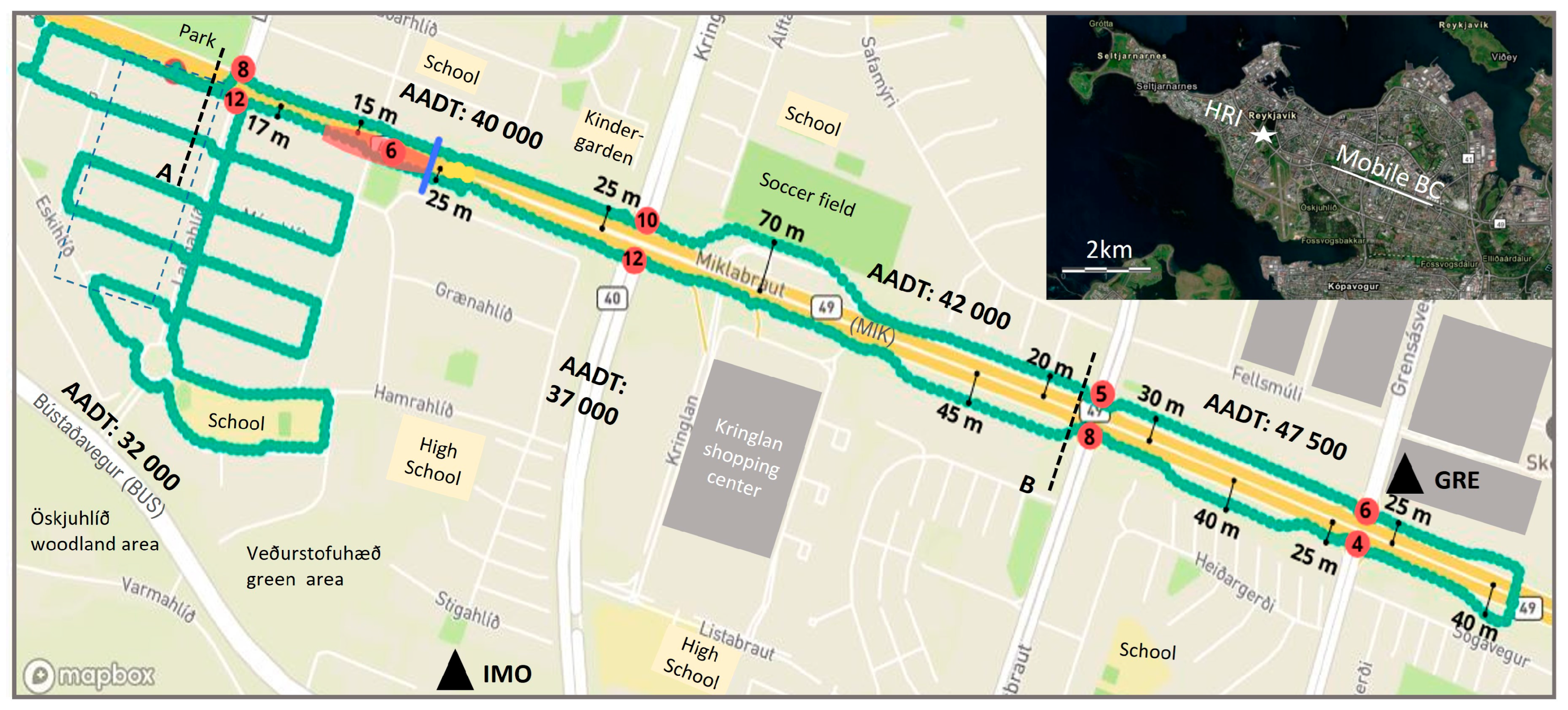
• Walking Highway (WH): Walking along a 2.2 km section of the MIK highway to resolve the spatial variability and potential exposure of pedestrians and cyclists. The traffic varied from 40,000 to 47,500 vehicles per day, and the canyon width ranged from 50 to 160 m. The walking path meandered along the highway, being both next to the curb and as far as 70 m from the centerline, and sometimes on the inside of a side berm for acoustic protection (Figure 2b,c). The long-term urban traffic station GRE was located 80 m from the centerline of the highway on a secondary artery.
• Walking Residential (WR): Walking within an adjacent residential neighborhood to assess the spatial reach of the traffic-related pollution, the urban background level and potential residential exposure. The Hlíðar neighborhood was chosen as the highway canyon was at its narrowest (Figure 1), and because the residential streets were parallel to the highway, allowing the assessment of a concentration profile with distance from the highway.
• Driving Highway (DH): Driving along the same 2.2 km section of highway to capture pollution levels closest to the source (aka tailpipe of vehicles) and the potential exposure of commuting by personal car.

The average monitoring time was 80 min, 44 min and 10 min for walking highway, walking residential, and driving highway routes, respectively. This corresponds to 4800, 2640 and 600 observations along the three routes. The instrument was warmed up for 30 min prior to use, then mounted in a stroller with the intake placed at 150 cm above ground to sample air at breathing level during walking campaigns. The instrument was thereafter placed in the front passenger seat of a 2009 Ford Focus model with a gasoline engine and a standard cabin filter designed to remove dust and pollen. The windows were kept closed, and the air conditioner was adjusted to high heat and medium ventilation, as is common in winter.

2.3. Reference Data

Hourly average air quality at the Grensás urban traffic monitoring station (GRE, 64.130° N, −21.875° W; in µg/m³) was obtained from the Environment Agency Iceland [32]. PM₁₀ with BAM 1020 was obtained using Met One Instruments (Grants Pass, OR, USA), while nitrogen oxides and sulfuric gases were obtained using a Thermo 42iQ NO-NO₂-NOx Analyzer and Thermo 450iQ H₂S-SO₂ Analyzer, respectively (Thermo Scientific, Waltham, MA, USA). Hourly average PM₁₀ and NO₂ levels at the HRI station were constructed from drift-corrected, 30-min measurements with a Continuous Particulate Monitor FH 62 C14 and 42iQ NO-NO₂-NOx Analyzer (Thermo Scientific, Waltham, MA, USA; retrieved from https://loftgaedi.is (accessed on 20 December 2017)).

Meteorological data from Reykjavík was obtained from the Icelandic Meteorological Office [33]. This consisted of 10-min averages recorded on the hour: air temperature (T, °C), wind speed at 10 m distance from the ground (W₁₀, m/s), wind direction (WD, degrees) and relative humidity (RH, %). In addition, hourly total short-wave radiation reaching the ground surface was received (Rad, W/m²), along with accumulated precipitation (P, mm/h) [33,34].

An independent estimate of near-surface atmospheric stability was derived from the high-altitude, low-resolution atmospheric sounding data measured at Keflavík airport by the Icelandic Meteorological Office (http://weather.uwyo.edu/upperair/sounding.html, accessed on 21 June 2023). Recordings were made at noon and midnight, and/or at 6 AM and 6 PM (in February and March). Data were missing for 28 December, 18–25 and 30–31 January. Since traffic-related BC was emitted and monitored within 1.5 m above ground, this study focused on the temperature gradient (or lapse rate, dT/dz, °C/m) between ground elevation (54 m above sea level) and the nearest observation, 50% of which were within 48 m elevation from the ground (interquartile range 83 m). A database of near-surface temperature gradients at noon and midnight was compiled for the study period from 27 October 2017 to April 09, 2018 (88% complete). An hourly database was constructed by linear interpolation between the bi-daily values.

Hourly traffic-count data for the measuring campaigns was obtained by request from the Icelandic Road Administration [35,36]. Traffic data was not fully reliable for the last three measurement days in spring. The data did not include breakdowns by vehicle type, but on average, heavy-duty vehicles represent 5% of the car fleet. Diesel vehicles accounted for ~40% of the car fleet and total driven kilometers in 2018 [25].

2.4. Data Preparation

Black Carbon (‘BC’) was taken at the 880 nm reading. To limit the impact of errors or outliers, the hourly average BC was calculated from the 1 min data at the stationary HRI site. In turn, the median, mean, standard deviation (S.D.) and interquartile range were estimated for each mobile campaign along each route. The mean BC can be interpreted as the average personal exposure during the route/transport mode taken. But in this study, the median BC was preferred as it is a more conservative estimate and can be interpreted as a spatial average concentration that is more representative, as it is less influenced by short-duration peaks associated with individual highly polluting vehicles (such as large, old diesel cars) either passing by or waiting at traffic lights. Negative BC values were included in the analyses as they reflect instrumental noise, and deleting them might bias the results.

Explanatory variables for the hourly BC during the stationary campaign were taken as the hourly reference data (see Section 2.3). Precipitation was categorized as rain or snow using the temperature threshold that incorporates relative humidity (RH), as given by [37].

$$T_{RH}=0.75+0.085\times (100\mathrm{\%}-RH)$$

(1)

If the air temperature exceeded T_RH, the recorded precipitation was assumed to be rain (wet), otherwise snow (dry).

Explanatory variables for the median BC monitored from the start to end of each mobile campaign were obtained as follows: For meteorological observations reported on the hour, the value corresponding to the median timing of the campaign was obtained by linear interpolation. For observations corresponding to accumulated or mean value within one hour (e.g., traffic volume and air quality), the observation within the hour during which most of the campaign was undertaken was used. If data was missing within that hour, an average of the hours before or after was taken. For the low temporal resolution atmospheric sounding data, the lapse rate was estimated with linear interpolation at 9 AM and 5 PM to represent the morning and afternoon rush-hour measurements.

2.5. Data Analyses

Linear regression analyses were performed on the hourly BC data from the stationary HRI site using Matlab (Mathworks Inc., Natic, MA, USA) to determine the primary indicators for the observed temporal variability in BC concentration. First, the Pearson correlation coefficient between BC and each external indicator (i.e., weather, traffic volume, ambient air quality) was assessed. The statistical significance of the correlation was assessed with the p-value. A correlation was deemed statistically significant if p < 0.05. Then, the slopes and intercepts were calculated for selected indicators, including their 95% confidence intervals (CI). Upon verifying that the intercepts of BC with traffic volume and the primary air quality indicator passed through zero, the final presentation of the regression lines was forced through zero to ease interpretation. The linear analyses were repeated on subsets of the HRI data, and on the median concentration from the mobile trips, to check for consistency.

Multi-regression analyses were performed to assess whether the prediction power of a linear model would be improved by adding more explanatory variables ($BC={\alpha }_0+{\alpha }_1{x}_1+{\alpha }_2{x}_2+{\alpha }_3{x}_3$ …). Parameters that did not significantly enhance the model performance were excluded from the analysis.

Given the strong linear regression relationship between mobile BC and NO₂ monitored at the stationary GRE station, time adjustment factors were calculated to account for the different gas pollution during the Walk Residential and Drive Highway (i = WR, DH) campaigns in relation to the Walk Highway campaign (WH), i.e.,

$${TAF}_i=\frac{{NO}_{2.WH}}{{NO}_{2,i}}$$

(2)

The time-adjusted BC concentration was then taken as ${TAF}_i\times {BC}_i$, which allowed comparison of the results from the three routes that were monitored in sequence.

Spatial variability was plotted on a Google map using the code by Bar-Yehuda [38]. Urban background (UB) was estimated as the median of BC concentration within a 120 m by 225 m section of the Hlíðar residential area with limited traffic influence. The UB definition of Boniardi et al. [39] was adopted, that is an area that was at a >75 m distance from the MIK Highway (>10,000 vehicles per day) and >50 m distance from the Langahlíð artery crossing the neighborhood (>1000 vehicles per day).

Concentration gradients were calculated as the difference between the median BC within each parallel street within the urban background area and the distance between streets. The half-concentration distance was assessed by fitting the BC concentration gradient to an exponential curve (e.g., [40]), after subtracting any asymptotic value within the neighborhood, defined as the lowest 5-percentile of measurements within the residential walking route. This value was zero except on two winter afternoons (13 December and 19 January), when it was 2 µg/m³. The gradients were classified based on the transport regime into the neighborhood, defined from the wind-speed component perpendicular to the MIK Highway,

$$W_{in}=W_{10}\times \mathrm{s}\mathrm{i}\mathrm{n}\left(\mathsf{\Delta }WD\right)$$

(3)

where $\mathsf{\Delta }WD$ is the relative angle between recorded wind direction and alignment of highway (292°). Three regimes were considered using the same threshold as [37]: downwind $W_{in}$ > 0.5 m/s, upwind $W_{in}$ < −0.5 m/s, and calm/parallel wind if −0.5 m/s < $W_{in}$ < 0.5 m/s.

3. Results and Discussion

3.1. Overview of Winter and Spring Season

To set the study results in context, the weather and air quality conditions at noon in Reykjavík City during the 2017–2018 study period (heavy line, dots or bars, Figure 3) are presented together with the range monitored in the years 2010–2018 (gray shade, Figure 3a–c,f–g). The peak winter months, from mid-November to mid-February, are characterized by very weak incoming solar radiation (<150 W/m², Figure 3a). The noontime air temperature fluctuates between −6 °C and +10 °C, and wind speeds average ~5 m/s (Figure 3b,c). The atmosphere can become very stable even during the daytime so that the air temperature increases with distance from the ground (positive near-surface dT/dz, Figure 3d). The boundary layer thickness can be as low as 10 m, as compared to >1 km in spring. Precipitation is frequent and mild, both in the form of rain and snow, with dry periods typically lasting no longer than 1–2 weeks (Figure 3e). Hourly nitrogen dioxide at noon can surpass the hourly health safety limit of 200 µg/m³ at this time (Figure 3f), even on wet days. PM₁₀ is also elevated (Figure 3g), but mostly on dry days, as rainfall and snow are effective in reducing PM₁₀ levels [41].

In springtime, with rising sun and air temperatures, the air becomes almost exclusively neutral or unstable (Figure 3d). Hourly nitrogen dioxide and particulate matter levels recorded at noontime rarely exceed 100 µg/m³ after mid-March (Figure 3f,g). As the roads dry up, the road and tire wear particles generated from the prevalent use of studded tires in the winter can be whirled up when the cars drive on dry roads, causing particulate matter episodes [42]. Dust can also be transported from the sandy regions, some 200+ km to the east of Reykjavík, or longer-range from other continents [26].

3.2. Stationary Campaign Summary

The stationary campaign from 27 October to 20 November captured the range in air temperature and wind speed in winter well (Figure 3b,c). The period was characterized by steady cooling and almost daily precipitation (<10 mm/day), both in the form of rain and snow (Figure 3d). BC was on average 1.0 ± 1.1 µg/m³ (maximum hourly average = 6.4 µg/m³; median = 0.6 µg/m³; interquartile range = 1.1 µg/m³). BC followed a strong diurnal cycle, with peaks aligning well with morning and afternoon rush-hour traffic (Figure 4). The morning rush hour started at 7 AM and peaked between 8 and 9 AM. The afternoon traffic was slightly higher, peaking around 5 PM on both weekdays and weekends. BC levels dropped to almost zero at night on weekdays, confirming that traffic is the main source of BC in this area, which includes both institutions and residences (Figure 2a), and that biomass burning is minimal, as expected in a city with geothermal district heating. Considerable weekend traffic and BC were detected, which can be explained by the proximity to the city center and the fact that throughflow traffic to the edge of the peninsula tends to become bottlenecked at the HRI site (Figure 1).

3.3. Mobile Campaign Summary

The mobile campaigns were conducted during rush hour on dry working days, targeting a wide range of traffic-related BC concentrations (Figure 3e). The dry period in the aftermath of the extreme pollution on New Year’s Eve 2017/2018 [43] was excluded to avoid firework-related BC. The statistical summary of the BC data monitored on the three routes, together with ambient air quality at the GRE Urban Traffic station, is presented in

Table 1. Summary statistics of BC measured on three routes (WH = Walk Highway; WR = Walk Residential; DH = Drive Highway). Also shown are the Time Adjustment Factors [TAF, see Equation (2)] and the average ambient air quality at the GRE station during rush hour (8 to 11 AM, 4 to 7 PM).

				Median (Mean ± S.D.) Uncorrected BC			TAF		GRE Station
				WH	WR	DH	WR	DH	NO2	PM10
Season	Mo.	Day	Time	(µg/m3)	(µg/m3)	(µg/m3)	(-)	(-)	(µg/m3)	(µg/m3)
Winter (N = 12)	12	13	MRH	2.9 (4.1 ± 5.0)	1.9 (1.9 ± 1.1)	4.1 (4.1 ± 0.8)	0.61	0.70	102 *	18
	12	13	ARH	8.8 (9.6 ± 5.4)	4.7 (5.1 ± 1.8)	11.4 (10.0 ± 4.7)	0.98	1.19	209 *	35
	12	14	MRH	6.3 (7.8 ± 5.6)	-	7.0 (7.8 ± 2.3)	-	0.99	174 *	24
	12	14	ARH	6.9 (8.0 ± 5.9)	3.0 (3.2 ± 1.3)	6.0 (6.3 ± 2.7)	0.94	0.94	211 *	28
	12	15	MRH	3.6 (4.6 ± 4.8)	0.3 (0.6 ± 1.7)	2.7 (2.8 ± 1.0)	1.19	1.12	129 *	10
	12	15	ARH	3.9 (4.5 ± 3.2)	2.1 (2.4 ± 1.6)	3.2 (3.8 ± 1.9)	1.41	1.17	121 *	12
	1	16	MRH	0.3 (0.9 ± 2.3)	0.1 (0.1 ± 0.4)	0.9 (1.3 ± 1.2)	1.48	1.48	37	10
	1	18	MRH	2.8 (3.6 ± 3.0)	0.9 (1.6 ± 2.6)	2.6 (3.4 ± 2.2)	1.01	2.06	90 *	12
	1	18	ARH	2.9 (3.7 ± 3.3)	1.5 (2.3 ± 3.0)	3.7 (3.8 ± 2.7)	0.61	0.58	94 *	11
	1	19	ARH	5.7 (6.2 ± 3.2)	4.5 (5.0 ± 2.3)	5.2 (5.3 ± 0.7)	0.99	0.88	203 *	27
	2	1	MRH	1.7 (2.7 ± 3.5)	0.7 (1.0 ± 0.9)	3.2 (3.4 ± 2.1)	0.97	1.26	85	6
	2	1	ARH	1.2 (2.4 ± 6.1)	0.3 (0.4 ± 0.5)	1.3 (1.6 ± 1.2)	1.09	1.09	29	9
Spring (N = 8)	3	1	MRH	0.6 (1.2 ± 2.3)	0.3 (0.4 ± 0.7)	2.3 (3.7 ± 3.9)	1.16	1.13	20	21
	3	1	ARH	1.7 (2.5 ± 2.9)	0.8 (1.0 ± 0.8)	5.3 (5.7 ± 2.7)	0.75	0.82	54	67 *
	3	2	MRH	3.6 (4.2 ± 2.7)	1.0 (1.8 ± 4.8)	2.8 (3.2 ± 1.1)	1.20	1.20	123	199 *
	3	2	ARH	1.2 (1.8 ± 2.3)	0.3 (0.6 ± 2.1)	1.6 (1.6 ± 1.3)	1.80	1.53	28	97 *
	3	23	ARH	1.0 (2.1 ± 3.9)	0.5 (0.7 ± 2.4)	3.0 (3.2 ± 1.3)	1.43	1.92	49	42
	4	3	ARH	0.9 (1.6 ± 2.7)	0.3 (0.8 ± 1.9)	2.1 (3.5 ± 3.3)	1.01	1.01	22	29
	4	9	MRH	1.4 (1.7 ± 1.6)	0.5 (0.6 ± 0.7)	2.4 (2.8 ± 1.5)	1.80	2.24	21	29 *
	4	9	ARH	1.0 (1.5 ± 1.7)	0.8 (0.8 ± 0.6)	1.5 (1.6 ± 0.7)	1.34	1.34	29	112 *

Notes: M/ARH = Morning/Afternoon Rush Hour * Exceeds the 24 h national air quality concentration limit (75 and 50 µg/m³ for NO₂ and PM₁₀, respectively).

. The winter campaigns were all conducted during stable atmospheric conditions (temperature gradient between +0.003 and +0.14 °C/m, Figure 3d). All but two of the measurement days were NO₂ episodes, on the basis that the national 24 h concentration limit for NO₂ was exceeded (75 µg/m³; [27,28]). Moreover, the hourly concentration limit (200 µg/m³) was exceeded on three monitored afternoons (Table 1). The BC levels recorded while walking along the GRE highway slightly surpassed the range measured at the stationary HRI site (Figure 3e), which is consistent with higher levels of traffic along the walking route than at the stationary site (43,000 vs. 28,000 vehicles/day) and higher atmospheric stability during peak winter. Conversely, the spring campaigns were conducted during neutral or moderately unstable atmospheric conditions (temperature gradient between −0.007 and −0.03 °C/m, Figure 3d). BC levels were more moderate on the walking routes when compared to winter, which is consistent with more efficient atmospheric mixing during unstable and neutral conditions, as previously noted with NO₂ and PM₁₀ (Figure 3f,g). Two monitoring days exceeded the 24 h concentration limit for PM₁₀ of 50 µg/m³. March 2 was attributed to local traffic and road dust, while April 9 was due to long-range transport from the east of Reykjavík, according to Environment Agency Iceland [28].

After adjusting the median BC to the timing of the WH campaign (Equation (2), Table 1), the average BC in winter was 4.6 ± 3.3 µg/m³, 3.9 ± 2.5 µg/m³ and 1.7 ± 1.6 µg/m³ while driving along the highway, walking along the highway and walking in a residential neighborhood, respectively (Figure 5a). Similarly, the average levels of BC in spring were 3.5 ± 1.5 µg/m³ (DH), 1.4 ± 0.9 µg/m³ (WH), and 0.7 ± 0.3 µg/m³ (WR, Figure 5b). The high BC levels while driving along the highway reflect the proximity to the source of traffic-related pollution, the limited initial mixing, and the limited protection provided by the vehicle. While these results conform with several earlier studies (e.g., [44,45]), the vehicle used for monitoring in this study was a 2009 model equipped with a standard cabin air filter designed to trap dust and pollen particulates in the 5–100 µm range, as opposed to ultra-fine particles such as BC. Today, High Efficiency Particulate Air (HEPA) filters are available that can trap 99% of 0.3 µm particles. Within-vehicle exposure for particles and gases can also be reduced by closing windows and keeping air conditioning on the “circulate” setting [46,47]. The low BC concentration further from the highway (WH, WR) reflects more effective atmospheric mixing during neutral or moderately unstable air in spring.

3.4. Linear Regression Analyses

The correlation of BC with explanatory variables is summarized in

Table 2. Pearson correlation coefficients (r) between BC concentration and external conditions during stationary (hourly average BC) and mobile campaigns (median BC).

			Stationary		Mobile
External Conditions	Parameter	Unit	All (N = 563)	9 AM-7 PM (N = 259)	WH (N = 20)	WR (N = 19)	DH (N = 20)
Traffic	Volume	veh./h	0.55 ***	0.29 ***	0.09	0.38	0.19
Weather	dT/dz	°C/m	0.17 ***	0.19 **	0.80 ***	0.67 **	0.64 **
	Tair	°C	−0.09 *	−0.10	−0.40	−0.34	−0.18
	W10	m/s	−0.36 ***	−0.45 ***	−0.67 **	−0.64 **	−0.73 ***
	WD	°	0.04	0.07	−0.05	0.01	0.05
	RH	%	0.04	0.15 *	0.40	0.40	0.35
	Rad	W/m2	0.11 *	−0.16 *	−0.46 *	−0.38	−0.30
	Rain	mm/h	−0.13 **	−0.19 **	-	-	-
	Snow	mm/h	0.04	0.06	-	-	-
Stationary	NO2	µg/m3	0.84 *** (2)	0.82 *** (2)	0.96 ***	0.88 ***	0.75 ***
Air Quality (1)	SO2	µg/m3	-	-	0.94 ***	0.85 ***	0.73 ***
	PM10	µg/m3	0.40 *** (2)	0.37 *** (2)	−0.02	−0.09	−0.11
	PM2.5	µg/m3	0.15 **	−0.03	0.03	−0.16	−0.21

Notes: Statistically significant correlation is noted by * p < 0.05 ** p < 0.01 *** p < 0.001. ⁽¹⁾ Air quality monitored at GRE unless otherwise specified; ⁽²⁾ Monitored at HRI.

(and Tables S1 and S2, in Supplementary Materials). Traffic was the strongest driver of the diurnal variability in BC at the stationary HRI site (Table 2, far left column). BC levels were less positively correlated to traffic during work hours and mobile rush-hour campaigns, as to be expected when neglecting times with no traffic. The ratio of BC in relation to daily traffic volume was consistently ~0.6 µg BC per 1000 vehicles per hour (

Table 3. Statistically significant linear regression slopes between BC and traffic volumes (µg BC per 1000 vehicles per hour) and NO₂ (µg/µg), assuming intercept is zero.

	Stationary			Mobile
Parameter	<Nov. 6	Nov. 6–12	Nov. 14–20	WH	WR	DH
Traffic vol.	0.57 ***	0.57 ***	0.61 ***	-	-	-
NO2	0.048 ***	0.035 ***	0.039 ***	0.032 ***	0.016 ***	0.035 ***

Notes: *** p < 0.001.

) throughout the 3-week monitoring period at the stationary HRI site. The intercept was not statistically significant and centered around zero (Table S3).

Atmospheric lapse rate and wind speed were identified as the primary meteorological drivers for the observed variability of BC, both in the stationary and mobile campaigns (Table 2). Both parameters improved the predictive power of the linear regression model incorporating traffic volume (ΔR² = +0.07 and +0.09, Table S5). High BC concentrations were associated with stable air (positive dT/dz), while low BC concentrations were associated with neutral or unstable air. A statistically significant negative relationship was also found between BC and wind speed. The positive relationship between urban BC levels and wintertime atmospheric stability and the negative relationship with wind speed conform to other studies (e.g., [11,12,21]). BC was negatively correlated with solar radiation and air temperature, suggesting both can be used as indicators for elevated traffic-related BC in the absence of lapse rate measurements. BC was negatively correlated with rainfall within the hour of observation at a statistically significant level, but this was not the case for snowfall. Generally, precipitation reduces particulate pollution, while its effect on gases such as NOx compounds is not as clear [41]. The addition of precipitation did not significantly improve the predictive power of the linear regression model incorporating traffic, lapse rate and wind speed (Table S5), as it was strongly correlated to wind speed (Table S1). Similarly, the non-statistical significant positive relationship between BC and relative humidity (as found in other studies, e.g., [45]) can be explained by the fact that relative humidity was correlated to other atmospheric indicators (e.g., lapse rate, Table S1), conforming to the finding of Liu et al. [21].

BC was strongly and positively correlated with nitrogen dioxide and sulfur dioxide during all campaigns (Table 2; Figure 6a). The correlation coefficient was somewhat stronger than reported in previous mobile studies (e.g., [45]), which can be explained by the BC source in this study being predominantly traffic-related and the monitoring focused on high-pollution days (Table 1; Figure 3f,g). The intercept passed through zero except for the Drive Highway campaign (Tables S3 and S4). The mass ratios of BC to NO₂ were consistent in time and space in the close vicinity of the highway (Table 3). The mass ratio was, on average, 50% less in the residential area 300 m from a major urban highway (compare WR to WH in Table 3).

While PM₁₀ was correlated with BC during the stationary campaign (Table 2), it did not improve the predictive power of the linear model already established between BC and NO₂ (Table S5). The mobile data rather suggests a bi-polar relationship between BC and particulate matter (Figure 6b,c): During the winter, BC constituted ~25% of the mass of PM_2.5, which is consistent with the BC/PM_2.5 ratio associated with fossil fuel burning in a Helsinki street canyon in winter [48]. In spring, BC represented only ~2% of the mass of PM_2.5 in accordance with local road dust, or alternatively long-transport dust, which contributed significantly to particles in the small diameter ranges [42,49].

3.5. Inner-City Spatial Variations

In spring (Figure 7a), elevated BC was observed on the outbound traffic lane at locations where vehicles idle, such as intersections, which is consistent with previous literature (e.g., [17]). BC infiltrated only the first street parallel to the highway. In winter (Figure 7b, top), however, very high BC pollution was measured along half of the walking and bike paths. Particularly noteworthy were the high BC concentrations along a 500 m section westward from the GRE urban air quality station, on the inner side of an earth berm designed for noise reduction (e.g., Figure 2c). BC levels tended to improve with distance from the highway, e.g., opposite the Kringlan shopping mall, where the walking path is 70 m from the centerline (Figure 1). Nevertheless, BC pollution penetrated the entire Hlíðar residential neighborhood (Figure 7b, bottom). The minimum concentration measured in the neighborhood on this day was 1.8 µg/m³, three times higher than the median BC measured 3 m from the roadside at the stationary HRI (Figure 4 and text therein). BC pollution infiltrated the neighborhood via transverse arteries or the open park area (green area, east of the study area). Lastly, elevated BC was also measured on the first street parallel to the highway in the south (Bústaðavegur), which suggests it may be a secondary source of traffic-related BC in the neighborhood.

3.6. Residential BC

The infiltration of BC into a residential area with limited direct traffic influence (dashed box, Figure 7b) is explored in Figure 8. BC concentration dropped with distance downwind into the neighborhood (Figure 8a), in accordance with the Gaussian Plume theory. Yet traffic-related BC matching or exceeding the median value near the roadside at the stationary HRI site (>1 µg/m³) was noted as far as 300 m from the neighborhood, both during mornings and afternoons on cold, dark days in December and January. At worst, a high, uniform BC concentration was observed in the entire neighborhood on cold winter afternoons with limited wind (Figure 8b). While such non-Gaussian distributions have been associated with oblique low wind impinging on moving vehicles and causing a vertical lift during unstable atmospheric conditions [11], it is more likely that in this study, vertical (atmospheric stability) and lateral (hillside) barriers trapped the pollution within the neighborhood, promoting buildup over the course of the work day. The Bústaðavegur (BUS) Highway located at the far end (x ≈ 0.5 km, Figure 7b) may also be contributing to pollution within the neighborhood, as indicated by the baseline concentration during upwind conditions (Figure 8c). Note that 9 April was a long-range transport PM episode, according to local authorities [28]. Excluding campaigns with low concentrations or missing data nearest to the source, half-concentration distances ranged from 45 to 200 m, a somewhat longer distance than the average 33 m recorded with stationary BC instruments over a two-week period in Helsinki, Finland, at the end of October [9].

Adopting the Urban Background (UB) definition of Boniardi et al. [39], which is >50 m and >75 m distance to a minor or major highway (dashed box, Figure 7b), the highest concentrations of ~5 µg/m³ in the residential neighborhood in this study match the maximum hourly UB values recorded in cities of greater size and more diverse sources of BC (

Table 4. Urban background levels of optical BC (µg/m³) during cold seasons in selected cities of increasing size and decreasing latitude.

City/Country	Lat. (°N)	BC Source	Monitoring Period	Tair (°C)	BC (µg/m3) Max. (Median)	Data Origin
Reykjavík/Iceland	64	T	MRH and ARH 13 December–9 April	−6 to +6	4.9	This study
Helsinki/Finland	60	FF	Jan.	−9	3.7 * (0.6)	[48]
		T	November–March	−15 to +9	2.4 * (0.65 **)	[50]
Milan/Italy	45	T, HH	MRH (7–9 AM)	3 to 10	4.3 (3.9)	[39]
			7 January–12 February	3 to 10	3.2 (3.0)

Notes: T = Traffic; FF = Fossil Fuel, HH = Household Heating; M/ARH = Morning/Afternoon Rush Hour; * 95 percentile hour (as opposed to maximum hour) ** Mean (as opposed to median).

). The median UB during peak winter is, in turn, arguably lower than the median roadside BC recorded at the stationary HRI site over a three-week period in November (0.6 µg/m³, see Section 3.2). As this value compares well to the median BC apportioned to fossil fuel combustion at UB sites in European cities such as Helsinki (Table 4), Birmingham, Zurich and Bern in winter [22], the median winter UB is likely to be lower in Reykjavík than in many other cities in more densely populated regions.

4. Final Remarks

This is the first BC monitoring study conducted in Iceland. In light of the good average urban air quality in this sparsely populated island nation, the research focused on characterizing the upper range of BC concentrations that the general public could be exposed to during rush-hour traffic in the vicinity and along a central highway in the capital city of Reykjavík. Unlike many studied urban sites in Europe [22], the contribution of residential and commercial wood and coal burning is negligible in winter, as both district heating and electricity are provided by renewable geothermal and hydropower resources. With only 230,000 inhabitants, the city is smaller than most previously studied urban areas. Even so, this study exhibited the detrimental effects of cold climate atmospheric stability on traffic-related BC pollution infiltrating residential neighborhoods. High urban background BC developed during frost stills when a positive atmospheric lapse rate was measured within 10–100 m from the ground. The highest residential concentrations monitored in this study matched or exceeded the worst urban background levels recorded in cities with over a million residents and diverse sources of BC (Table 4). The pollution penetrated deep into the residential neighborhoods, with BC levels > 2 µg/m³ recorded at >300 m distance from the 43,000 vehicles per day traffic source (Figure 7). Residential homes, children’s schools, recreational areas and sports areas are sited within that distance from the studied highway (Figure 1), suggesting that sensitive groups would be exposed episodically to high BC levels on such cold, still winter days.

This study also indicated that commuting via driving, walking or cycling along an urban highway can cause significant BC exposure, even in small communities. The key reason is the high volume of traffic along the studied highway, partially due to the consolidation of traffic along main arteries to the city center—which is sited at the tip of a peninsula (Figure 1)—and partially due to the high rate of personal car ownership in Iceland (767 vehicles per 1000 inhabitants in 2018 [25]). The average BC during the walk highway campaigns in winter and spring (2.3 µg/m³; 43,000 vehicles per day) was thus slightly higher than in similar campaigns along roads with lower traffic in Stockholm (1.2–1.8 µg/m³; <30,000 vehicles per day [45]). In accordance with the existing literature, the highest BC levels were recorded at intersections, pedestrian crossings and bus stops, where traffic slows down. BC exceeded 10 µg/m³ at these “hot spots” during 20–60% of the campaigns (Figure 1 top, orange) targeting medium to high ambient air pollution. A more novel finding in this study is that earth berms for noise reduction did not protect pedestrians and cyclists from the ultrafine BC pollution.

NO₂ monitored at an urban traffic site was found to be a reliable indicator of BC levels within 300 m of the highway (Table 2, Figure 6a); both NO₂ and BC are generated by incomplete burning of fuel, and BC is an ultrafine particle. The ratio of BC to NO₂ was consistent over time and at various locations close to the highway (Table 3). The publicly available real-time monitoring of NO₂ in Reykjavík can thus be used as a proxy for BC pollution in wintertime near major urban traffic arteries. The study also confirmed the presence of significant non-combustion-related sources of particulate matter in a cold climate, such as local road dust generated by the prevalent use of studded tires and long-range dust, which reduces the ratio of BC to PM₁₀ (and PM_2.5) in spring. Traffic volume, wind speed and atmospheric lapse rate were the three key explanatory variables for the variability in hourly BC concentration (Table 2).

The study was limited to one instrument, targeting days with high pollution. This limited the number of mobile campaigns and the possibility of synchronous campaigns. Reference traffic and PM_2.5 data were missing during some mobile campaigns, and the atmospheric sounding data had low vertical (>20 m) and time (12 h) resolution. Despite these limitations, the key findings were consistent within the study and compared well with other studies. In the future, it is important to perform continuous, long-term measurements in order to assess trends in air quality and the effect of emission mitigation actions [51]. Such actions may include diverting the highest emitters of BC, heavy-duty vehicles and diesel passenger cars, from the most central city artery, where many pedestrians, cyclists and residents may be exposed to traffic-related BC, as well as making active transport modes more competitive with the personal car.

References

1. Europe’s Air Quality Status 2023. Available online: https://www.eea.europa.eu/publications/europes-air-quality-status-2023 (accessed on 21 June 2023).
2. European Environment Agency [EEA]. Air Quality in Europe—2020 Report; Publications Office of the European Union: Luxembourg, 2020. [Google Scholar]
3. Park, M.; Joo, H.S.; Lee, K.; Jang, M.; Kim, S.D.; Kim, I.; Borlaza, L.J.S.; Lim, H.; Shin, H.; Chung, K.H.; et al. Differential Toxicities of Fine Particulate Matters from Various Sources. Sci. Rep. 2018, 8, 17007. [Google Scholar] [CrossRef]
4. Janssen, N.A.H.; Gerlofs-Nijland, M.E.; Lanki, T.; Salonen, R.O.; Cassee, F.; Hoek, G.; Fischer, P.; Brunekreef, B.; Krzyzanowski, M. Health Effects of Black Carbon; World Health Organization [WHO]—Regional Office for Europe: Copenhagen, Denmark, 2012. [Google Scholar]
5. Samoli, E.; Atkinson, R.W.; Analitis, A.; Fuller, G.W.; Green, D.C.; Mudway, I.; Anderson, H.R.; Kelly, F.J. Associations of Short-Term Exposure to Traffic-Related Air Pollution with Cardiovascular and Respiratory Hospital Admissions in London, UK. Occup. Environ. Med. 2016, 73, 300–307. [Google Scholar] [CrossRef] [PubMed]
6. Atkinson, R.W.; Analitis, A.; Samoli, E.; Fuller, G.W.; Green, D.C.; Mudway, I.S.; Anderson, H.R.; Kelly, F.J. Short-Term Exposure to Traffic-Related Air Pollution and Daily Mortality in London, UK. J. Expo. Sci. Environ. Epidemiol. 2016, 26, 125–132. [Google Scholar] [CrossRef] [PubMed]
7. Schwartz, J.; Bind, M.-A.; Koutrakis, P. Estimating Causal Effects of Local Air Pollution on Daily Deaths: Effect of Low Levels. Environ. Health Perspect. 2017, 125, 23–29. [Google Scholar] [CrossRef] [PubMed]
8. World Health Organization. WHO Global Air Quality Guidelines: Particulate Matter (PM2.5 and PM10), Ozone, Nitrogen Dioxide, Sulfur Dioxide and Carbon Monoxide; World Health Organization: Geneva, Switzerland, 2021; ISBN 978-92-4-003422-8. [Google Scholar]
9. Enroth, J.; Saarikoski, S.; Niemi, J.; Kousa, A.; Ježek, I.; Močnik, G.; Carbone, S.; Kuuluvainen, H.; Rönkkö, T.; Hillamo, R.; et al. Chemical and Physical Characterization of Traffic Particles in Four Different Highway Environments in the Helsinki Metropolitan Area. Atmos. Chem. Phys. 2016, 16, 5497–5512. [Google Scholar] [CrossRef]
10. Wiesner, A.; Pfeifer, S.; Merkel, M.; Tuch, T.; Weinhold, K.; Wiedensohler, A. Real World Vehicle Emission Factors for Black Carbon Derived from Longterm In-Situ Measurements and Inverse Modelling. Atmosphere 2021, 12, 31. [Google Scholar] [CrossRef]
11. Liang, M.S.; Keener, T.C.; Birch, M.E.; Baldauf, R.; Neal, J.; Yang, Y.J. Low-Wind and Other Microclimatic Factors in near-Road Black Carbon Variability: A Case Study and Assessment Implications. Atmos. Environ. 2013, 80, 204–215. [Google Scholar] [CrossRef]
12. Chen, Y.; Schleicher, N.; Fricker, M.; Cen, K.; Liu, X.-L.; Kaminski, U.; Yu, Y.; Wu, X.-F.; Norra, S. Long-Term Variation of Black Carbon and PM2.5 in Beijing, China with Respect to Meteorological Conditions and Governmental Measures. Environ. Pollut. 2016, 212, 269–278. [Google Scholar] [CrossRef]
13. Segersson, D.; Eneroth, K.; Gidhagen, L.; Johansson, C.; Omstedt, G.; Nylén, A.E.; Forsberg, B. Health Impact of PM10, PM2.5 and Black Carbon Exposure Due to Different Source Sectors in Stockholm, Gothenburg and Umea, Sweden. Int. J. Environ. Res. Public Health 2017, 14, 742. [Google Scholar] [CrossRef]
14. Chambliss, S.E.; Preble, C.V.; Caubel, J.J.; Cados, T.; Messier, K.P.; Alvarez, R.A.; LaFranchi, B.; Lunden, M.; Marshall, J.D.; Szpiro, A.A.; et al. Comparison of Mobile and Fixed-Site Black Carbon Measurements for High-Resolution Urban Pollution Mapping. Environ. Sci. Technol. 2020, 54, 7848–7857. [Google Scholar] [CrossRef]
15. Tessum, M.W.; Sheppard, L.; Larson, T.V.; Gould, T.R.; Kaufman, J.D.; Vedal, S. Improving Air Pollution Predictions of Long-Term Exposure Using Short-Term Mobile and Stationary Monitoring in Two US Metropolitan Regions. Environ. Sci. Technol. 2021, 55, 3530–3538. [Google Scholar] [CrossRef]
16. Van den Hove, A.; Verwaeren, J.; Van den Bossche, J.; Theunis, J.; De Baets, B. Development of a Land Use Regression Model for Black Carbon Using Mobile Monitoring Data and Its Application to Pollution-Avoiding Routing. Environ. Res. 2020, 183, 108619. [Google Scholar] [CrossRef]
17. Dons, E.; Panis, L.I.; Poppel, M.V.; Theunis, J.; Wets, G. Personal Exposure to Black Carbon in Transport Microenvironments. Atmos. Environ. 2012, 55, 392–398. [Google Scholar] [CrossRef]
18. Rivas, I.; Donaire-Gonzalez, D.; Bouso, L.; Esnaola, M.; Pandolfi, M.; de Castro, M.; Viana, M.; Àlvarez-Pedrerol, M.; Nieuwenhuijsen, M.; Alastuey, A.; et al. Spatiotemporally Resolved Black Carbon Concentration, Schoolchildren’s Exposure and Dose in Barcelona. Indoor Air 2016, 26, 391–402. [Google Scholar] [CrossRef] [PubMed]
19. Janhäll, S.; Olofson, K.F.G.; Andersson, P.U.; Pettersson, J.B.C.; Hallquist, M. Evolution of the Urban Aerosol during Winter Temperature Inversion Episodes. Atmos. Environ. 2006, 40, 5355–5366. [Google Scholar] [CrossRef]
20. Olofson, K.F.G.; Andersson, P.U.; Hallquist, M.; Ljungström, E.; Tang, L.; Chen, D.; Pettersson, J.B.C. Urban Aerosol Evolution and Particle Formation during Wintertime Temperature Inversions. Atmos. Environ. 2009, 43, 340–346. [Google Scholar] [CrossRef]
21. Liu, B.; Ma, Y.; Gong, W.; Zhang, M.; Shi, Y. The Relationship between Black Carbon and Atmospheric Boundary Layer Height. Atmos. Pollut. Res. 2019, 10, 65–72. [Google Scholar] [CrossRef]
22. Savadkoohi, M.; Pandolfi, M.; Reche, C.; Niemi, J.V.; Mooibroek, D.; Titos, G.; Green, D.C.; Tremper, A.H.; Hueglin, C.; Liakakou, E.; et al. The Variability of Mass Concentrations and Source Apportionment Analysis of Equivalent Black Carbon across Urban Europe. Environ. Int. 2023, 178, 108081. [Google Scholar] [CrossRef] [PubMed]
23. Environment Agency Iceland [EIA]. Informative Inventory Report: Emissions of Air Pollutants in Iceland from 1990 to 2021; Umhverfisstofnun: Reykjavík, Iceland, 2023. [Google Scholar]
24. Andradóttir, H.Ó.; Hjartardóttir, B. Sót í Reykjavík—Forrannsókn (English: Black Carbon in Reykjavík—Pilot Study); University of Iceland: Reykjavík, Iceland, 2018. [Google Scholar]
25. Icelandic Transport Authority. Traffic Statistics by Type of Car, Type of Fuel. Available online: https://island.is/oennur-toelfraedi-samgoengustofu (accessed on 21 June 2023).
26. Thorsteinsson, T.; Gísladóttir, G.; Bullard, J.; McTainsh, G. Dust Storm Contributions to Airborne Particulate Matter in Reykjavík, Iceland. Atmos. Environ. 2011, 45, 5924–5933. [Google Scholar] [CrossRef]
27. Environment Agency Iceland [EIA]. Loftgæði á Íslandi—Ársskýrsla 2017 (English: Air Quality in Iceland—Annual Report 2017); Umhverfisstofnun: Reykjavík, Iceland, 2019. [Google Scholar]
28. Environment Agency Iceland [EIA]. Loftgæði á Íslandi—Ársskýrsla 2018 (English: Air Quality in Iceland—Annual Report 2018); Umhverfisstofnun: Reykjavík, Iceland, 2020. [Google Scholar]
29. Höskuldsson, P.; Thorlacius, A. Uppruni svifryks í Reykjavík (English: Particle Matter Sources in Icleand); Efla Consulting: Reykjavík, Iceland, 2017. [Google Scholar]
30. Mendoza, D.L.; Hill, L.D.; Blair, J.; Crosman, E.T. A Long-Term Comparison between the AethLabs MA350 and Aerosol Magee Scientific AE33 Black Carbon Monitors in the Greater Salt Lake City Metropolitan Area. Sensors 2024, 24, 965. [Google Scholar] [CrossRef] [PubMed]
31. Holder, A.; Seay, B.; Brashear, A.; Yelveton, T.; Blair, J.; Blair, S. Evaluation of a Multi-Wavelength Black Carbon (BC) Sensor; Clean Air Society of Australia and New Zealand: Melbourne, Australia, 2018. [Google Scholar]
32. Environment Agency Iceland [EIA]. Air Quality Data Grensás Urban Traffic Site from 2010 to 2019; Environment Agency Iceland [EIA]: Reykjavík, Iceland, 2023. [Google Scholar]
33. Icelandic Meteorological Office [IMO]. Hourly Weather and Rain at Reykjavík Automatic Station Nr. 1475 From1997 to 2019; Icelandic Meteorological Office [IMO]: Reykjavík, Iceland, 2020. [Google Scholar]
34. Icelandic Meteorological Office [IMO]. Hourly Radiation and Soil Temperature in Reykjavík; Icelandic Meteorological Office [IMO]: Reykjavík, Iceland, 2019. [Google Scholar]
35. Icelandic Road Administration [IRA]. Traffic Counts on Miklabraut during Mobile Monitoring Campaigns; Icelandic Road Administration [IRA]: Reykjavík, Iceland, 2018. [Google Scholar]
36. Icelandic Road Administration [IRA]. Traffic Counts on Hringbraut Section Nr. 49-05 Eastbound and Section Nr. 49-04 Westbound; Icelandic Road Administration [IRA]: Reykjavík, Iceland, 2023. [Google Scholar]
37. Feiccabrino, J.; Graff, W.; Lundberg, A.; Sandström, N.; Gustafsson, D. Meteorological Knowledge Useful for the Improvement of Snow Rain Separation in Surface Based Models. Hydrology 2015, 2, 266–288. [Google Scholar] [CrossRef]
38. Bar-Yehuda, Z. Matlab Function for Plotting a Google Map on the Background of a Figure. Available online: https://github.com/zoharby/plot_google_map (accessed on 21 June 2022).
39. Boniardi, L.; Dons, E.; Campo, L.; Van Poppel, M.; Int Panis, L.; Fustinoni, S. Annual, Seasonal, and Morning Rush Hour Land Use Regression Models for Black Carbon in a School Catchment Area of Milan, Italy. Environ. Res. 2019, 176, 108520. [Google Scholar] [CrossRef] [PubMed]
40. Zhu, Y.; Hinds, W.C.; Kim, S.; Shen, S.; Sioutas, C. Study of Ultrafine Particles near a Major Highway with Heavy-Duty Diesel Traffic. Atmos. Environ. 2002, 36, 4323–4335. [Google Scholar] [CrossRef]
41. Aldrin, M.; Haff, I.H. Generalised Additive Modelling of Air Pollution, Traffic Volume and Meteorology. Atmos. Environ. 2005, 39, 2145–2155. [Google Scholar] [CrossRef]
42. Barr, B.C.; Andradóttir, H.Ó.; Thorsteinsson, T.; Erlingsson, S. Mitigation of Suspendable Road Dust in a Subpolar, Oceanic Climate. Sustainability 2021, 13, 9607. [Google Scholar] [CrossRef]
43. Andradottir, H.O.; Thorsteinsson, T. Repeated Extreme Particulate Matter Episodes Due to Fireworks in Iceland and Stakeholders’ Response. J. Clean. Prod. 2019, 236, 117511. [Google Scholar] [CrossRef]
44. Okokon, E.O.; Yli-Tuomi, T.; Turunen, A.W.; Taimisto, P.; Pennanen, A.; Vouitsis, I.; Samaras, Z.; Voogt, M.; Keuken, M.; Lanki, T. Particulates and Noise Exposure during Bicycle, Bus and Car Commuting: A Study in Three European Cities. Environ. Res. 2017, 154, 181–189. [Google Scholar] [CrossRef] [PubMed]
45. Merritt, A.-S.; Georgellis, A.; Andersson, N.; Bero Bedada, G.; Bellander, T.; Johansson, C. Personal Exposure to Black Carbon in Stockholm, Using Different Intra-Urban Transport Modes. Sci. Total Environ. 2019, 674, 279–287. [Google Scholar] [CrossRef]
46. Matthaios, V.N.; Kramer, L.J.; Crilley, L.R.; Sommariva, R.; Pope, F.D.; Bloss, W.J. Quantification of Within-Vehicle Exposure to NOx and Particles: Variation with Outside Air Quality, Route Choice and Ventilation Options. Atmos. Environ. 2020, 240, 117810. [Google Scholar] [CrossRef]
47. Campagnolo, D.; Borghi, F.; Fanti, G.; Keller, M.; Rovelli, S.; Spinazzè, A.; Cattaneo, A.; Cavallo, D.M. Factors Affecting In-Vehicle Exposure to Traffic-Related Air Pollutants: A Review. Atmos. Environ. 2023, 295, 119560. [Google Scholar] [CrossRef]
48. Helin, A.; Niemi, J.V.; Virkkula, A.; Pirjola, L.; Teinilä, K.; Backman, J.; Aurela, M.; Saarikoski, S.; Rönkkö, T.; Asmi, E.; et al. Characteristics and Source Apportionment of Black Carbon in the Helsinki Metropolitan Area, Finland. Atmos. Environ. 2018, 190, 87–98. [Google Scholar] [CrossRef]
49. Lundberg, J.; Gustafsson, M.; Janhäll, S.; Eriksson, O.; Blomqvist, G.; Erlingsson, S. Temporal Variation of Road Dust Load and Its Size Distribution—A Comparative Study of a Porous and a Dense Pavement. Water Air Soil Pollut. 2020, 231, 561. [Google Scholar] [CrossRef]
50. Luoma, K.; Niemi, J.V.; Aurela, M.; Fung, P.L.; Helin, A.; Hussein, T.; Kangas, L.; Kousa, A.; Rönkkö, T.; Timonen, H.; et al. Spatiotemporal Variation and Trends in Equivalent Black Carbon in the Helsinki Metropolitan Area in Finland. Atmospheric Chem. Phys. 2021, 21, 1173–1189. [Google Scholar] [CrossRef]
51. Friman, M.; Aurela, M.; Saarnio, K.; Teinilä, K.; Kesti, J.; Harni, S.D.; Saarikoski, S.; Hyvärinen, A.; Timonen, H. Long-Term Characterization of Organic and Elemental Carbon at Three Different Background Areas in Northern Europe. Atmos. Environ. 2023, 310, 119953. [Google Scholar] [CrossRef]
Figure 1. Aerial photo of Reykjavík peninsula with a City Center–HRI stationary monitoring site (white star; insert) and closeup of the mobile walking routes along the MIK highway and inside residential Hlíðar neighborhood (green dots). Annual Average Daily Traffic [AADT], distance to centerline of highway and land activities are indicated on the map: Schools (yellow), parks and sporting fields (green), commercial areas (gray), pedestrian crossing lights (blue line), official weather and air quality monitoring sites (triangles). Frequency of hot spots (>10 µg/m3 BC) are noted in orange circles.
Atmosphere 15 00312 g001
Figure 2. Highway transects facing west: (a) Stationary site (canyon width 50 ± 10 m); (b) Residential Hlíðar neighborhood with public park to the right (canyon width 55 ± 10 m); (c) Near Kringlan Shopping Center (canyon width ranges 60–155 m).
Atmosphere 15 00312 g002
Figure 3. Noontime atmospheric conditions during the study period from 27 October 2017 to 9 April 2018 (line) in relation to the historical range (2010–2018, shade): (a) global radiation; (b) air temperature; (c) wind speed; (d) atmospheric lapse rate; (e) black carbon at HRI, during walk highway campaigns and during diurnal precipitation; (f) nitrogen dioxide, and (g) particulate matter (PM10) at the GRE urban traffic station.
Atmosphere 15 00312 g003
Figure 4. Diurnal variations at the HRI stationary site: (a) black carbon; (b) traffic volumes. The central mark indicates the median value within the hour and the edges of the box represent the interquartile range. The whiskers extend to the most extreme data points not considered outliers. The ‘+’ marker symbol represent outliers. M/ARH = Morning/Afternoon Rush Hour.
Atmosphere 15 00312 g004
Figure 5. Distribution of time-adjusted median BC during the drive highway (DH), walk highway (WH) and walk residential (WR) mobile campaigns in Reykjavík City during (a) winter (b) spring. The central mark indicates the median value and the edges of the box represent the interquartile range. The whiskers extend to the most extreme data points not considered outliers (marked as ‘+’).
Atmosphere 15 00312 g005
Figure 6. Relationship between BC along highway and ambient air quality: (a) NO2; (b) PM10; (c) PM2.5. Stationary BC represents hourly measurements from 27 October to 20 November (N = 563); Mobile BC are medians while walking along the highway (WH). Linear regression (LR) lines are forced through zero.
Atmosphere 15 00312 g006
Figure 7. Spatial distribution of BC when walking along MIK highway (top) and in the Hlíðar residential neighborhood (bottom) during (a) spring dust and (b) winter BC episodes. Dashed gray lines delineate the urban background area used for calculating concentration profiles.
Atmosphere 15 00312 g007
Figure 8. Median BC concentration along 120 m long sections of roads in residential neighborhoods, classified according to transport regimes: (a) wind directed from BUS highway into neighborhood, Win < −0.5 m/s; (b) wind from MIK highway into neighborhood, Win > 0.5 m/s; (c) parallel or no wind. Dot sizes represent wind speed, W10.
Atmosphere 15 00312 g008