Abstract
Arizona, a rapidly growing state in the southwestern U.S., faces ozone pollution challenges, including nonattainment areas in Yuma and Maricopa counties influenced by neighboring state pollution transport. In this study, we use five-year (2017–2021) hourly back-trajectories and O3 concentration data for concentration-weighted trajectory (CWT) analysis to identify transport pathways and potential source regions of O3 at six monitoring sites in Arizona. We divide the data into five seasons (winter, spring, dry summer, monsoon summer, and fall) to examine variations in O3 concentration and transport across sites and seasons. The highest mean O3 concentrations occur during spring (37–49 ppb), dry summer (39–51 ppb), and monsoon summer (34–49 ppb), while winter (19–41 ppb) exhibits the lowest seasonal mean. The CWT results reveal that high O3 concentrations (≥40 ppb) in Arizona, with the exception of Phoenix and Tucson sites, are influenced significantly by regional and international transport, especially in spring (14.9–35.4%) and dry summer (12.7–26.9%). The major potential source areas (excluding the Phoenix and Tucson sites) are predominantly located outside Arizona. This study highlights the critical role of pollution transport in influencing O3 variability within Arizona and will be valuable in shaping pollution control strategies in the future.
1. Introduction
Tropospheric ozone (O3) is an important agent in atmospheric chemistry and elevated levels promote adverse effects on human health [1,2,3], crops, and natural vegetation [4,5,6,7,8]. Exposure to increased levels of O3 is associated with reduced lung function [9], airway inflammation [10,11], asthma incidence and premature deaths [1]. Furthermore, elevated O3 can also impact vegetation by reducing carbon uptake and decreasing crop yields [12]. Ground level O3 is a by-product of the reactions between hydroxyl radicals (OH), volatile organic compounds (VOCs), and oxides of nitrogen (NOx = NO + NO2) in the presence of sunlight [13,14,15]. The variability of O3 levels is influenced by several factors including local chemistry [16,17], meteorology [18,19,20], and transport [21,22,23,24,25]. The lifetime of O3 can vary from a few hours to a few weeks [26] with a globally averaged lifetime of ~22–23 days [27,28] allowing transport for long distances [24]. For example, the transport of pollution from East Asia contributes to the background O3 concentration across the western U.S. [29,30]. Jacob et al. [29] predicted a monthly mean increase in O3 concentrations by 2–6 ppbv in the western U.S. as a result of the tripling of Asian anthropogenic emissions from 1985 to 2010. Fiore et al. [31] reported that the background O3 produced outside the North American boundary layer contributes an average of 25–35 ppbv to summer afternoon O3 concentrations in surface air in the western United States. McDonald-Buller et al. [32] and Jaffe et al. [33] also noted that spring and summer background O3 levels are most enhanced at high elevation locations in the western U.S.
One of the fastest growing areas of the U.S. is the state of Arizona, with its two most populated cities being Phoenix (>5 million; 20% population growth between 2010 and 2020) and Tucson (>1 million; 8% population growth between 2010 and 2020) [34]. Arizona is also home to several national parks where air monitoring is routinely conducted due to concerns regarding visibility and public health. Currently, parts of four counties (Gila, Maricopa, Pinal, Yuma) in Arizona are classified as O3 nonattainment areas. Specifically, Maricopa County falls under the Phoenix-Mesa moderate nonattainment area, while Yuma County is included in the Yuma marginal nonattainment area (https://www3.epa.gov/airquality/greenbook/jncs.html#AZ (accessed on 10 January 2024)). Arizona is one of many semi-arid/arid regions in the Southwest U.S., which are less commonly studied as it relates to ozone pollution. Not only that, but Arizona is an intriguing case to study also because of its complex terrain [35], significant urbanization, the influence of a summertime monsoon [36], wildfire activity [37], and being downwind of several O3 (and precursor) hotspot emissions from California and Mexico [38]. This combination of attributes makes it hard to generalize results from other areas and apply them to Arizona.
While the reader is referred elsewhere ([39] and references therein) for a detailed review of past O3-related work for Arizona, a brief mention is important that some of the works reviewed highlighted the likely importance of non-local source contributions to O3 from regional transport [40,41,42,43,44]. Qu et al. [44] reported that the majority of the ozone exceedance in Yuma, especially in summer, is associated with air masses coming from southern California and northern Mexico. In the spring months between 1996 and 2000, using back trajectories, Diem [42] demonstrated that the transport of O3 from California was responsible for Grand Canyon National Park’s elevated O3 level days. Analyzing kinematic back trajectories, Gaffney et al. [43] showed that O3 levels in Phoenix during summer are impacted by the transport of pollutants from cities such as Los Angeles and San Diego in California. Model simulation by Li et al. [45] found that the daily maximum 8-h average O3 level in the Phoenix metropolitan region was predominately affected by contributions from local emissions in Arizona, but there is still a sizable contribution (ranging from a few ppb to over 30 ppb) from southern California. Combining ground-based measurement, remote sensing, and model simulations, Huang et al. [38] analyzed the effect of southern California (SoCal) anthropogenic emissions on O3 pollution in the southwestern U.S. and found that the transported pollution from SoCal contributed up to 15 ppb in western Arizona. Many of these studies mentioned influences from California and Mexico.
Our study distinguishes itself by conducting a detailed analysis of transport pathways impacting O3 at different sites around Arizona and for various times of the year, with a particular focus on dividing the summer into its dry and monsoon components. We employed concentration-weighted trajectory (CWT) analysis [46,47] to study transport pathways and potential source areas affecting O3 at six sites across Arizona using data from 2017 to 2021. The structure of the paper is as follows: (i) discussion of methods, (ii) summary of meteorological conditions and back trajectories affecting the study sites, (iii) overview of seasonal profile of O3 concentration, (iv) discussion of the seasonal CWT profiles of O3, (v) and conclusions. The results help to better understand the causes of O3 pollution and provide guidance for pollution control strategies in the region.
2. Methods
2.1. Site Descriptions
Six monitoring sites (Figure 1) were strategically chosen to study the influence of pollution transport, following past studies conducted in these locations, and to represent rural and urban areas in the region. Site details (Table 1) were obtained from the United States Environmental Protection Agency Air Quality System (US EPA AQS; https://aqs.epa.gov/aqsweb/airdata/download_files.html (accessed on 11 August 2023)).
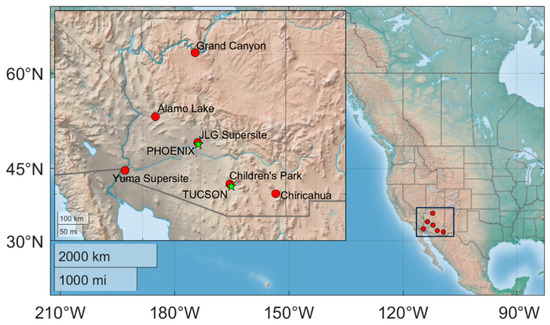
Figure 1.
Map showing the locations of the O3 monitoring sites (red circles). The Chiricahua and Grand Canyon stations are operated by the National Park Service; the Alamo Lake, JLG Supersite, and Yuma Supersite by the Arizona Department of Environmental Quality (ADEQ); and the Children’s Park by the Pima County Department of Environmental Quality. Green stars are placed by Arizona’s two major cities, Tucson and Phoenix.

Table 1.
Details of each O3 monitoring site in Arizona.
Grand Canyon National Park is a high-elevation ozone monitoring station and is considered a rural site, with Class 1 (i.e., requires a high level of air quality protection) airshed designation under the U.S. Clean Air Act (https://www.nps.gov/chir/learn/nature/airquality.htm (accessed on 10 January 2024)). Despite its rural classification, it is one of the most visited parks in the country, with an annual average visitation of ~5.2 million during the study period (National Park Service, 2023). Past studies related to this site investigated stratospheric ozone intrusion [48,49] as well as the transport of pollution from California [42]. Alamo Lake is located in Alamo Lake State Park with the surrounding area consisting mostly of desert. Alamo Lake is considered a background site and is identified by ADEQ as a regional transport site for O3. It is located to the northwest (and generally upwind) of the Phoenix metropolitan area, with the nearest traffic corridor around 80 km away. JLG Supersite was established to monitor air quality in the Phoenix Metropolitan area’s central core. It is a designated National Core (NCore) monitoring station. NCore is a multi-pollutant network that integrates various instruments to measure pollutant gases, aerosols, and meteorological variables (https://www.epa.gov/amtic/ncore-monitoring-network (accessed on 7 July 2023)). JLG Supersite is situated in a valley [35] with the surrounding area primarily residential and is impacted by urban pollution [50,51] as well as pollution transport from California [43,45]. Yuma Supersite is located near the California border on the west and U.S.-Mexico border on the south and southwest and is impacted by both local as well as regional pollution transport from northern Mexico [44]. The surrounding area is commercial and industrial and is located in an urban city center. Both Yuma Supersite (Yuma County) and JLG Supersite (Maricopa County) are part of an 8-h O3 nonattainment area (https://azdeq.gov/nonattainment_areas (accessed on 1 August 2023)). Children’s Park is also part of the NCore monitoring network and is representative of a residential area located at an urban and city center. Children’s Park is influenced by transport from Phoenix, as well as from Texas and Mexico [52]. We note that Children’s Park is not considered the site with the maximum O3 concentration in Pima County; rather, it serves as a site for population exposure monitoring. Chiricahua National Monument is a relatively remote site located in the Chiricahua Mountains of southeastern Arizona, also with Class 1 airshed designation. The monument’s relatively close proximity (~79 km) to the U.S.-Mexico border makes it a good site to study the possible transport of pollution from Mexico.
2.2. Surface O3 Measurements
Hourly O3 data from 1 January 2017 to 31 December 2021 were obtained from the U.S. EPA AQS website (https://aqs.epa.gov/aqsweb/airdata/download_files.html (accessed on 19 November 2022)). Chiricahua and Grand Canyon are part of the U.S. Clean Air Status and Trends Network (CASTNET), a multi-pollutant monitoring network designed to monitor regional air quality (https://www.epa.gov/castnet (accessed on 11 August 2023)). CASTNET provides data in rural areas not monitored by the State and Local Air Monitoring Sites (SLAMS) network. Alamo Lake and Yuma Supersite are part of the SLAMS network, which also includes stations classified as NCore (JLG Supersite, Children’s Park). CASTNET and SLAMS measure O3 using ultraviolet (UV) absorbance with Federal Equivalent Method (FEM) compliant monitors. For this study, quality control was applied to the raw data before doing further analysis. Zero and negative values were treated as missing [53,54] while values below the method detection limit (MDL: 5 ppb) were replaced with 0.5 × MDL [55]. The number of BDL, negative, and zero values are summarized in Table S1. On average, the pandemic did not significantly impact data completeness, likely because the instrumentation did not involve extensive manual labor.
2.3. Additional Data
Hourly meteorological data (temperature, wind speed, wind direction, and relative humidity) are used from the US EPA website for Grand Canyon, JLG Supersite, Children’s Park, and Chiricahua (https://aqs.epa.gov/aqsweb/airdata/download_files.html (accessed on 19 May 2023)). For the Yuma Supersite, data from a secondary monitoring station (Yuma Valley, 5.9 km away) were downloaded from the Arizona Meteorological Network (AZMET) website (https://ag.arizona.edu/azmet/ (accessed on 10 April 2023)). Monthly planetary boundary layer height (PBLH) data were obtained from the Modern Era-Retrospective Analysis for Research and Applications (MERRA-2) model with 0.5° × 0.625° spatial resolution [56]. Fire radiative power (FRP) data were downloaded from the NASA Fire Information for Resource Management System (FIRMS; https://earthdata.nasa.gov/firms (accessed on 12 April 2023)) from 2017–2021. Only the FRP data with a high detection confidence level (≥80%) were used, as recommended in the MODIS user’s guide [57].
2.4. Air Mass Trajectory Analysis
To track air masses arriving at the monitoring sites, four-day (96 h) back trajectories were generated using the NOAA HYSPLIT model [58,59]. Trajectories were calculated using the Global Data Assimilation System (GDAS) 1° resolution data and the “model vertical velocity” method at 500 m (a.g.l) arrival height. While we acknowledge the advantage of using higher-resolution data, given our focus on long-range and regional transport, we find the use of GDAS data acceptable in this context. That being said, we conducted a sensitivity analysis for a representative year (2021) for a single site (Alamo Lake) and concluded that the general seasonal trends in trajectories are preserved when comparing GDAS to 12 km data from the North American Mesoscale Forecast System (NAM) (Figure S1). Furthermore, we did sensitivity tests for that same year and site to see the level of change from using different ending altitudes (10 m and 100 m) and also when using nighttime trajectories versus those in the daytime; the results showed no major differences in overall results (Figures S2 and S3). Future work can further explore sensitivity analysis using different meteorological datasets. The choice of 500 m as the ending altitude represents the mixed layer used by related surface air quality studies [60,61,62].
Hourly trajectories were generated for each day (a total of 24 trajectories per day) between 1 January 2017 and 31 December 2021 to match the hourly O3 data. To categorize the trajectory data into distinct classes, cluster analysis was performed using the HYSPLIT model, and details of the clustering algorithm can be found in Stunder [63]. The four-day back trajectories, resolved into 3 h points, were used for the analysis per site and season. In the clustering process, the spatial variance (SV) was estimated between each endpoint along each trajectory within a cluster, and the sum of all SV is considered as the cluster spatial variance (CSV). The clustering method also calculates the total spatial variance (TSV), which is the sum of the CSV over all clusters. The point just before the large increase in TSV gives the ideal final number of clusters [63].
2.5. Concentration-Weighted Trajectory (CWT) Analysis
Concentration-weighted trajectory (CWT) analysis was conducted to identify the potential source areas of O3 observed at the six monitoring sites. It assigns a weighted concentration to a grid (0.5° × 0.5°) by calculating the mean of sample concentrations with trajectories passing a certain cell in the grid (Equation (1)) [46,47] as follows:
where is the average weighted concentration in the th cell, is the index of trajectory, is the total number of trajectories, is the concentration observed on the arrival of trajectory , and is the time spent in the th cell by trajectory . An arbitrary weighting function (Equation (2)) was applied to the CWT O3 concentrations to minimize uncertainty associated with fewer trajectories [64,65,66,67].
To examine seasonality, the CWT profiles were divided into five seasons: winter (December–February), spring (March–May), dry summer (June), monsoon summer (July–August), and fall (September–November). A unique aspect of this study is the separation of the traditional summer season (June, July, and August) into two seasons (dry summer and monsoon summer) to separate the impact of the North American Monsoon (NAM), which ramps up in July and persists through August [68,69]. The TrajStat: GIS-based software [70] generated CWT profiles. The probability (Equation (3)), representing the residence time of trajectories associated with relatively high CWT values (≥40 ppb), was calculated using the following formula:
where is the number of trajectory segment endpoints that fell in the th cell, and is the total number of endpoints [71,72].
3. Results and Discussions
3.1. Seasonal Profiles
3.1.1. Meteorological Parameters
Meteorological profiles are first summarized to provide context to interpret O3 characteristics for the study region (Figure S4). The details of the dataset used are summarized in Section 2.3. Relative humidity (RH) is highest in winter and lowest in dry summer, while temperatures are lowest in winter and highest during dry and monsoon summers. Similar to temperature, the planetary boundary layer height (PBLH) shows a seasonal low during winter and a peak in both the dry and monsoon summers. Wind speed shows its highest values during spring at both Chiricahua and Grand Canyon, with a minimum during monsoon summer. At the JLG Supersite, Children’s Park, and Yuma Supersite, wind speed is at its highest during spring and monsoon summer and is lowest in winter. We note that the relative strength of the monsoon season can vary from year to year, resulting in changes in the meteorological profiles in the summer months.
3.1.2. Back Trajectories
We generated hourly four-day back trajectories (Figure S5) and divided them into five seasons to examine the role of seasonal changes in air mass patterns impacting surface O3 at the receptor sites. To simplify the trajectory results, Figure 2 shows the seasonal profile of cluster analysis color-coded by mean O3 concentration per cluster, while Table S2 summarizes the mean O3 concentrations and percentage of trajectories per cluster.
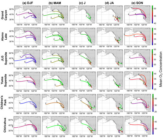
Figure 2.
Seasonal cluster mean trajectories are classified into 3–7 groups and color-coded by mean O3 concentrations. Clustering was performed on four-day back trajectories between 1 January 2017 and 31 December 2021.
Trajectories from winter to spring are predominantly westerly and northwesterly, with the majority of airmasses from over the Pacific Ocean (Figure S5). The trajectories suggest the role of long-range transport as shown by air masses coming from distant regions. Some trajectories even passed through Alaska and some parts of Canada. For each site, only one cluster was identified of continental origin accounting for 30–51% of trajectories. This cluster exhibits the lowest O3 mean at all sampling sites, except at JLG Supersite (Table S2). The presence of a southwesterly cluster was only observed at Chiricahua (44%). On average, longer clusters have higher mean O3, except at JLG Supersite and Children’s Park. During spring, clusters are still dominated by westerly-northwesterly flow but with more trajectories from shorter distances. At Grand Canyon, we identified a prominent southwesterly cluster (31%), while a northeasterly cluster (6%) was present at Chiricahua (Figure 2b). Trajectories generally transition from westerly-northwesterly to westerly-southwesterly during dry summer. Clusters coming from distant regions start to diminish in frequency during dry summer accounting for only a small portion (2–6%) of the trajectories (Figure 2c). At Children’s Park and Chiricahua, we observed clusters coming from the east, northeast, and southeastern parts of Arizona with higher mean O3 concentration, which is not evident at the four other locations.
Clusters during monsoon summer are particularly unique with the absence of clusters showing trajectories originating farther away from the sampling locations (Figure 2d). While the majority of trajectories come from areas outside Arizona, 14% (JLG Supersite) and 19% (Grand Canyon) of trajectories are from within Arizona within a four-day range. Due to the strengthening effect of the NAM, trajectories in monsoon summer become predominantly southerly-southwesterly. This motivates the importance for studies to avoid lumping June with the rest of the summer encompassing NAM as it mixes different predominant trajectory pathways, in addition to different meteorological conditions (Figure S4). Clusters with higher mean O3 concentration during this season are from the eastern side of the sampling sites, albeit with a lower percentage of total trajectories (Table S2). The fall season is characterized by trajectories from all directions, thus serving as a transition period between monsoon summer and winter. The fall season exhibits clusters again coming from distant areas but only accounting for a small portion of the total trajectories. However, these farther-reaching clusters exhibit higher mean O3 at three sampling sites (Grand Canyon Alamo Lake, Chiricahua) (Table S2). Clusters over land dominate during this season, but only Alamo Lake has a cluster (48%) from within Arizona (Figure 2e). These results demonstrate the importance of both long-range transports of pollutants within a four-day duration and also the temporal variability in transport corridors leading to this study’s receptor sites.
3.1.3. Surface O3 Concentrations
Previous works in Arizona demonstrated there is an impact of long-range transport on surface O3 concentration [30,42,44]. Here, we present the seasonal profile of O3 and subsequently discuss the influence of transport on the seasonality of O3 concentration.
Seasons with the highest mean seasonal concentrations of O3 (for both hourly and MDA8) are as follows for each site (Table 2): Grand Canyon, Alamo Lake, Children’s Park = dry summer; JLG Supersite = dry and monsoon summer; Yuma Supersite = spring and dry summer; Chiricahua = spring. For all sites, the lowest seasonal mean O3 concentrations were observed during winter (Figure 3), which has the farthest-reaching trajectories. The difference in seasonal trends between sites is presumed to be linked to their location and thus proximity to precursor emissions and major transport corridors.
Table 2.
Seasonal mean ± standard deviation of O3 concentrations (ppb) from hourly averaged data and MDA8 (in parenthesis). Seasons are defined as follows: winter (DJF), spring (MAM), dry summer (J), monsoon summer (JA), and fall (SON).
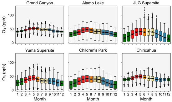
Figure 3.
Monthly profiles of hourly O3 concentrations from 1 January 2017 to 31 December 2021. Boxes represent the 25th–75th percentile (interquartile), and whiskers extend to 1.5× the interquartile range. The horizontal lines represent median values, black dots represent mean values, and black diamonds represent outliers. Boxplots are colored by season: DJF (green), MAM (red), J (orange), JA (khaki), and SON (steel blue).
Notable during the study period is the COVID-19 pandemic, which requires treatment in terms of how it affected this study’s results. On average during the year 2020 overlapping with the pandemic lockdown, we observe a reduction in O3 concentrations during the spring and summer months, in particular at Grand Canyon, JLG Supersite, and Yuma Supersite (Figure S6). The yearly mean O3 concentration did not vary that much (±2 ppb) before and during COVID-19 (summary table not shown).
Among the six sites considered in this study, only two sites (JLG Supersite and Children’s Park) have NOx and CO data available. An examination of CO and NOx data shows that higher O3 concentrations are linked to lower NOx and CO concentrations (Figure S7). Elevated NOx levels during winter and fall can cause O3 titration, which reduces O3 concentrations during these seasons [73]. It is important to note that VOC measurements in the region remain limited, highlighting a significant gap that needs to be addressed in the future [39].
A previous study conducted at Grand Canyon based on data collected from mid-April to mid-September in 2017, reported that VOC concentrations are lower compared to those observed in other national parks, likely due to the influence of long-range transport [48]. The recent study by Gou et al. [74] utilized the TROPOMI (Tropospheric Monitoring Instrument) formaldehyde (HCNO)-to-NO2 ratio (FNR) to show that central Phoenix is predominantly in the VOC-limited or transitional regime in June, with lower FNR in Phoenix compared to Tucson.
Higher O3 concentration during summer (especially dry summer) can be at least partly attributed to higher temperature [75], and lower RH [76,77,78] (Figure S4). Wise and Comrie [79] reported that O3 in Phoenix is mostly influenced by temperature, and their other study [80] identified mixing height as having the strongest influence on O3 formation and accumulation in Tucson. Diem and Comrie [52] also reported that the elevated O3 levels in August are in part due to the NAM. Meteorological conditions during winter (Figure S4) such as lower temperature and higher RH [78] are unfavorable for O3 formation and accumulation, hence lower O3 concentration during this season. While low temperatures may slow down the rate of O3 formation, it can still occur if sufficient amounts of NO2 and VOCs are present. The relationship between PBLH and surface ozone is complex and needs further analysis as PBLH can either counteract or enhance O3 reduction through dilution, depending on the O3 concentration in the entrained air [81].
3.2. Trajectory Patterns: CWT Profiles
The chosen method to couple the previous results shown independently for trajectories and O3 concentrations is CWT analysis, with seasonal results shown to provide evidence of the influence of the transport of pollution on the seasonality of O3 levels (Figure 4). While the cluster results discussed in Section 3.1.2 provide information on predominant pathways of air masses impacting the receptor sites, the CWT profiles determine the possible source locations of elevated O3 concentrations associated with those transport routes. The seasonal CWT profiles were color-coded based on the weighted O3 concentrations. We also plotted monthly CWT maps for all sites for one representative year (2021), which are provided in Figure S8. Table 3 additionally uses the seasonal CWT profiles to quantify the residence time of back trajectories with relatively high O3 (≥40 ppb) that are either inside or outside Arizona, with the latter category further divided into individual states, countries, and the Pacific Ocean in Table S3. Ideally, it would be preferable to use a threshold of >70 ppb for this analysis. However, the limited number of values above 70 ppb at most sites posed a challenge for conducting seasonal CWT runs (Table S4). The choice of 40 ppb as a threshold was based on visual inspection of the CWT maps (orange-red colors). We also experimented with a threshold of >50 ppb for the analysis and arrived at a similar conclusion, noting that the majority of these points were located outside Arizona (Table S3).
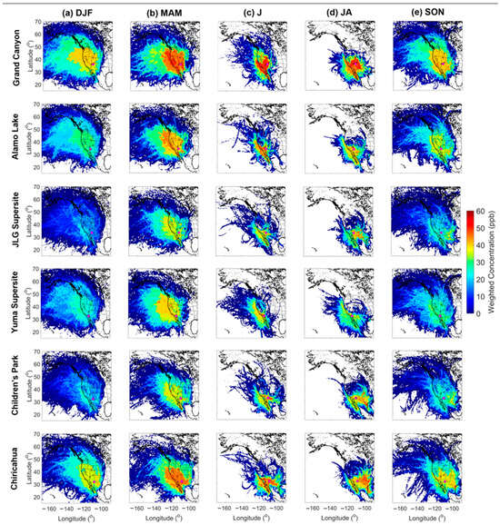
Figure 4.
Seasonal CWT profile for O3 based on four–day back trajectories with an ending altitude of 500 m above ground level at six sites between January 2017 and December 2021 for (a) DJF (winter), (b) MAM (spring), (c) J (dry summer), (d) JA (monsoon summer), and (e) SON (fall). The monthly CWT profile for each sampling site for one representative year (2021) is shown in Figure S8.
Table 3.
Percentage of residence time of trajectories associated with high O3 CWT values (≥40 ppb) within and outside Arizona, with the latter divided into continental (“Outside Arizona”) and marine (“Ocean”) regions. GC—Grand Canyon, AL—Alamo Lake, JS—JLG Supersite, YS—Yuma Supersite, CP—Children’s Park, and CM—Chiricahua. Blank cells represent no cases with O3 CWT values ≥ 40 ppb.
3.2.1. December–February (Winter)
The winter season (Figure 4a) exhibits the widest spatial range of potential source areas, although no distinct ‘hotspot’ is evident during this season. As discussed in Section 3.1.3, the seasonal mean of O3 concentrations at all sites is lowest during winter. Moreover, a majority of clusters identified during winter come from distant regions, mainly over the open ocean (Figure 2a). At Grand Canyon, air masses associated with high O3 concentrations predominantly arrive from the west-northwest regions. A similar pattern is observed at Alamo Lake, albeit with reduced O3 concentrations. At Grand Canyon, longer residence time associated with CWT values above 40 ppb was observed outside of Arizona, specifically in California, Utah, and Nevada (Table S5). A subtle difference between JLG Supersite and Children’s Park was observed, with Children’s Park having more influence from the southeast-northeastern direction, despite the cluster analysis not pinpointing a specific southeast-northeast cluster. Noteworthy is that a large percentage of trajectories at Children’s Park are from the west (51%) (Figure 2a), within the Arizona region, likely stemming from transport from the much larger Phoenix metropolitan area. Meanwhile, Chiricahua exhibits elevated O3 concentration from the southeast-northeast region, spanning southern parts of New Mexico, western Texas, and northern Mexico. Similar to Children’s Park, the cluster analysis for Chiricahua did not identify a specific southeast-northeast cluster. We note that only two sites (Grand Canyon and Chiricahua) have CWT values above 40 ppb, which are both dominated by trajectories outside of Arizona (35.1% and 6.0%) (Table 3).
3.2.2. March–May (Spring)
For spring (Figure 4b), the potential source regions for higher O3 concentrations are coming from all directions, especially west-northwest regions, including neighboring states of California, Nevada, and Utah, extending as far as Oregon and Washington, and south-southwest (Mexico). In particular, the CWT profile at Grand Canyon revealed multiple ‘hotspots’ associated with trajectories coming from California (including the San Diego area), and eastern parts of Arizona. The monthly CWT map for the year 2021 shows more hotspots in May compared to March and April (Figure S8e). A study by Diem [42] using spring month data between 1996 and 2000 further supports these findings, attributing the increased O3 level days in the Grand Canyon to the transport of pollutants from California. While CWT maps at the other five sites showed lower concentrations and fewer hotspots, their transport patterns resemble that of the Grand Canyon, except for elevated (≥40 ppb) O3 concentrations at Chiricahua from northern Mexico. Utilizing FIRMS data from 2017–2021, we generated seasonal fire radiative power (FRP) maps, which serve as a proxy for fire intensity [62,82,83,84]. The number of fires during spring is significantly higher than the other seasons, particularly in Mexico and the western regions of the U.S. Additionally, a significant number of fire spots are observed within the California and Arizona regions. Although outside the scope of this study, it is encouraged to further examine the effects of smoke events on O3 in Arizona and other parts of the desert southwestern U.S. Generally, the residence time of trajectories associated with CWT values ≥ 40 ppb is higher outside Arizona, ranging from 2.6–40.2% over continental and 3.7–35% over marine regions, compared to within Arizona where it ranges from 1–22.5% (Table 3). The residence times for each major potential source area are summarized in Table S5.
3.2.3. June (Dry Summer)
During the dry summer (Figure 4c), we observed more areas contributing to elevated O3 levels, especially at Grand Canyon. The major source areas impacting the Grand Canyon were dispersed from the north-northwest and south-southwest, encompassing the southern regions of California, Nevada, Utah, western parts of Arizona, and northern Mexico. The cluster results for Grand Canyon indicated that a substantial amount (56%) of trajectories (Figure 2c) come from Baja California, Mexico. Similar potential major source areas were identified for Alamo Lake, JLG Supersite, and Yuma Supersite, with the exception that these sites lack major source areas located to the north. At the Yuma Supersite, 46% of trajectories traveled near the California coastline, while 9% came from Mexico (Figure 2c). The residence times of air masses associated with high CWT values (≥40 ppb) were 7.0% for California and 9.3% for Mexico (Table S5). This aligns with previous work by Qu et al. [44] for Yuma, which showed that most O3 exceedances during summer are associated with back trajectories from southern California and the northern part of Mexico. For Children’s Park and Chiricahua, potential source areas were observed to the east-southeast, including the southern tip of New Mexico, and parts of El-Paso, Texas, and Ciudad Juarez, Mexico (Table S5). In the dry summer, we observe elevated fire intensity near Baja California, Mexico, and a significant number of fire spots in the western part of Mexico. These conditions have the potential to influence O3 levels in Arizona and thus warrant further investigation. In summary, during this season, the residence times of trajectories linked to high CWT values (≥40 ppb) are higher from areas outside of Arizona, with the exception of JLG Supersite and Children’s Park (Table 3). This implies that local O3 production still predominates at JLG Supersite and Children’s Park, which are located in urban areas.
3.2.4. July–August (Monsoon Summer)
During monsoon summer (Figure 4d), the CWT profile for all sites shows the narrowest spatial coverage of potential source areas indicating a more stagnant condition conducive to O3 buildup [85]. At Grand Canyon and Chiricahua, wind speeds were lowest in July and August (Figure S4). More areas located at the east-northeast and southeast directions contribute to elevated O3 concentration during monsoon summer compared to the dry summer period. In 2021, in general, higher CWT values were observed in July compared to August (Figure S8g). CWT results at Grand Canyon showed the highest concentrations coming from west-northwest, and east-southeast including parts of eastern California, southern Nevada, Utah, Arizona, and New Mexico. The CWT profile at the JLG supersite exhibited scattered hotspots located to the north, northeast, and southeast of the sampling site. As discussed in Section 3.1.2, despite the prevalence of clusters from areas outside Arizona, it is worth noting that 14% of trajectories at JLG Supersite (Figure 2d) are from within the Arizona region. Also important is the different CWT profile at Yuma Supersite (lower concentration and fewer potential source areas northeast of the sampling site) during this season compared to the other sites.
Children’s Park results reveal certain hotspots near Ciudad Juarez, Mexico, and El Paso, Texas. According to Diem and Comrie [52], transport from the El-Paso/Ciudad Juarez area contributes to elevated O3 concentrations in Tucson, particularly in August and September. For Chiricahua, there are significant potential source regions to the east and northeast, covering parts of southern New Mexico, northeastern Texas, and northern Mexico. The cluster results indicate that 23% of trajectories in Chiricahua are from the Texas area, while 65% come from Mexico (Figure 2d). In monsoon summer, the number of fires in Mexico significantly decreases compared to both spring and dry summer, indicating a reduced likelihood of contributing to the elevated O3 concentration associated with air masses coming from Mexico. Similarly, the number of fires in California is higher during this season. However, its potential impact is expected to be limited for the majority of the sites due to the absence of clusters passing through the California region, except at Grand Canyon (24%) and Alamo Lake (14%). Similar to dry summer, the percentage of residence time of trajectories associated with CWT values ≥ 40 ppb is highest outside of Arizona, except at Grand Canyon and JLG Supersite (Table 3).
3.2.5. September–November (Fall)
The fall (Figure 4e) and winter seasons showed similar transport patterns but fall exhibited a more dominant source region situated to the south-southeast part of the sampling sites. At Grand Canyon, the CWT map reveals potential source areas to the west and southeast of the sampling site. For JLG Supersite, Children’s Park, and Chiricahua, the CWT maps indicate potential source areas located east-southeast, encompassing the western part of Texas and the northeastern part of Mexico. Clustering results reveal trajectories coming from the east (Children’s Park = 16%, Chiricahua = 22%) and southeast (Yuma Supersite = 17%, JLG Supersite = 28%, Alamo Lake = 48%). We note that clusters over land dominate during this season. The majority of trajectories still come from outside Arizona, except for Alamo Lake having 48% of trajectories from within Arizona (Figure 2e). In general, the residence time of trajectories associated with high CWT values from outside Arizona dominates during this season (Table 3).
4. Conclusions
This study applied back trajectory clustering and CWT analysis to a five-year dataset to identify the transport pathways and potential source areas leading to elevated O3 concentrations measured at the six monitoring stations situated across rural and urban locations in Arizona. A novel aspect of this study was separating the analysis into five distinct seasons that take into account different meteorological conditions that can impact O3 formation and transport. We observed the highest mean O3 concentrations during spring, and dry and monsoon summers, while winter consistently displayed the lowest seasonal mean O3 concentrations across all sites. Seasonal variations in major potential source regions were evident, with relatively high CWT values in spring and summer months predominantly outside Arizona (with the exception of Phoenix and Tucson sites), most notably from California and Mexico. This observation aligns with previous studies (e.g., [38,42,43,44,45,52,86] which suggests that California and Mexico are contributors to elevated O3 levels in our study region.
While the CWT technique has been widely implemented in identifying the impact of long-range pollutant transport, it does not accurately pinpoint primary local sources of O3. Moreover, the lack of simultaneous NOx and VOC data limited our ability to trace the transport paths of these key O3 precursors to the study sites. Moving forward, we also encourage VOC measurements across Arizona and in-depth analysis of the impact of wildfires on elevated O3 concentrations across the southwestern U.S., building upon existing research in this area [39]. Future studies are encouraged using chemical transport modeling focusing on potential source areas identified in this study to accurately quantify the percentage contribution of pollution transport to elevated O3 concentration in the region. In addition, the spatio-temporal distribution of O3 precursors from point sources (including power plants) can be explored in the future [87].
Ultimately, this work motivates more attention towards controlling sources affecting high concentrations as identified particularly at the monitoring sites with especially higher concentrations, and hopefully, with increasing inventories of precursor (NOx and VOC) data, this can become easier over time.
Supplementary Materials
The following supporting information can be downloaded at: https://www.mdpi.com/article/10.3390/atmos15040401/s1, Figure S1: comparison of HYSPLIT back trajectories using NAM 12 km data and GDAS data; Figure S2: comparison of HYSPLIT back trajectories at different arrival heights at Alamo Lake; Figure S3: comparison of daytime and nighttime HYSPLIT back trajectories at 500 m level at Alamo Lake; Figure S4: monthly profile of surface meteorological data at six sites; Figure S5: HYSPLIT back trajectories at 500 m level over the six monitoring sites; Figure S6: monthly mean of hourly O3 concentrations between 2017 and 2021 at the six sampling sites; Figure S7: monthly profiles of NOx and CO concentrations at JLG Supersite and Children’s Park; Figure S8: monthly CWT maps for 2021; Table S1: summary of datapoints below detection limit, negative, and zero; Table S2: seasonal statistical result of hourly O3 for each trajectory cluster; Tables S3 and S5: residence time of trajectories associated with high O3 CWT values within and outside Arizona. Table S4: number of data points with values > 70 ppb.
Author Contributions
Conceptualization, methodology, G.B. and A.S.; formal analysis, and investigation, G.B.; writing—original draft preparation, G.B.; writing—review and editing, A.S. and A.A.; supervision, A.S.; funding acquisition, A.S. and A.A. All authors have read and agreed to the published version of the manuscript.
Funding
This research was funded by the Arizona Board of Regents (ABOR) Regent’s Grant from the Technology and Research Initiative Fund (TRIF).
Institutional Review Board Statement
Not applicable.
Informed Consent Statement
Not applicable.
Data Availability Statement
EPA: https://www.epa.gov/aqs (accessed on 19 November 2022). MODIS: https://earthdata.nasa.gov/firms (accessed on 12 April 2023). AZMET: https://ag.arizona.edu/azmet/ (accessed on 10 April 2023). NASA GES DISC: https://giovanni.gsfc.nasa.gov/ (accessed on 12 April 2023). HYSPLIT: http://ready.arl.noaa.gov (accessed on 22 December 2022).
Acknowledgments
We acknowledge the use of data from NASA’s Fire Information for Resource Management System (FIRMS) (https://earthdata.nasa.gov/firms (accessed on 12 April 2023)), part of NASA’s Earth Observing System Data and Information System (EOSDIS). The authors gratefully acknowledge the NOAA Air Resources Laboratory (ARL) for the provision of the HYSPLIT transport and dispersion model and READY website (https://www.ready.noaa.gov (accessed on 22 December 2022)) used in this publication. The authors acknowledge the EPA Air Quality Systems (AQS) database (https://www.epa.gov/aqs (accessed on 19 November 2022)). We gratefully acknowledge Connor Stahl and Hossein Dadashazar for their help and guidance with the CWT and back trajectory analysis.
Conflicts of Interest
The authors declare no conflicts of interest.
References
- Zhang, J.J.; Wei, Y.; Fang, Z. Ozone Pollution: A Major Health Hazard Worldwide. Front. Immunol. 2019, 10, 2518. [Google Scholar] [CrossRef]
- Nuvolone, D.; Petri, D.; Voller, F. The effects of ozone on human health. Environ. Sci. Pollut. Res. Int. 2018, 25, 8074–8088. [Google Scholar] [CrossRef]
- Smith, K.R.; Jerrett, M.; Anderson, H.R.; Burnett, R.T.; Stone, V.; Derwent, R.; Atkinson, R.W.; Cohen, A.; Shonkoff, S.B.; Krewski, D.; et al. Public health benefits of strategies to reduce greenhouse-gas emissions: Health implications of short-lived greenhouse pollutants. Lancet 2009, 374, 2091–2103. [Google Scholar] [CrossRef]
- Ainsworth, E.A.; Lemonnier, P.; Wedow, J.M. The influence of rising tropospheric carbon dioxide and ozone on plant productivity. Plant Biol. 2020, 22 (Suppl. 1), 5–11. [Google Scholar] [CrossRef]
- Agathokleous, E.; Feng, Z.; Oksanen, E.; Sicard, P.; Wang, Q.; Saitanis, C.J.; Araminiene, V.; Blande, J.D.; Hayes, F.; Calatayud, V.; et al. Ozone affects plant, insect, and soil microbial communities: A threat to terrestrial ecosystems and biodiversity. Sci. Adv. 2020, 6, eabc1176. [Google Scholar] [CrossRef]
- Tai, A.P.K.; Sadiq, M.; Pang, J.Y.S.; Yung, D.H.Y.; Feng, Z. Impacts of Surface Ozone Pollution on Global Crop Yields: Comparing Different Ozone Exposure Metrics and Incorporating Co-effects of CO2. Front. Sustain. Food Syst. 2021, 5, 534616. [Google Scholar] [CrossRef]
- Emberson, L.D.; Pleijel, H.; Ainsworth, E.A.; van den Berg, M.; Ren, W.; Osborne, S.; Mills, G.; Pandey, D.; Dentener, F.; Büker, P.; et al. Ozone effects on crops and consideration in crop models. Eur. J. Agron. 2018, 100, 19–34. [Google Scholar] [CrossRef]
- Grulke, N.E.; Heath, R.L. Ozone effects on plants in natural ecosystems. Plant Biol. 2020, 22 (Suppl. 1), 12–37. [Google Scholar] [CrossRef] [PubMed]
- Tager, I.B.; Balmes, J.; Lurmann, F.; Ngo, L.; Alcorn, S.; Kunzli, N. Chronic exposure to ambient ozone and lung function in young adults. Epidemiology 2005, 16, 751–759. [Google Scholar] [CrossRef] [PubMed]
- Jorres, R.A.; Holz, O.; Zachgo, W.; Timm, P.; Koschyk, S.; Muller, B.; Grimminger, F.; Seeger, W.; Kelly, F.J.; Dunster, C.; et al. The effect of repeated ozone exposures on inflammatory markers in bronchoalveolar lavage fluid and mucosal biopsies. Am. J. Respir. Crit. Care Med. 2000, 161, 1855–1861. [Google Scholar] [CrossRef] [PubMed]
- Kinney, P.L.; Nilsen, D.M.; Lippmann, M.; Brescia, M.; Gordon, T.; McGovern, T.; El-Fawal, H.; Devlin, R.B.; Rom, W.N. Biomarkers of lung inflammation in recreational joggers exposed to ozone. Am. J. Respir. Crit. Care Med. 1996, 154, 1430–1435. [Google Scholar] [CrossRef] [PubMed]
- Juráň, S.; Grace, J.; Urban, O. Temporal Changes in Ozone Concentrations and Their Impact on Vegetation. Atmosphere 2021, 12, 82. [Google Scholar] [CrossRef]
- Chameides, W.L.; Fehsenfeld, F.; Rodgers, M.O.; Cardelino, C.; Martinez, J.; Parrish, D.; Lonneman, W.; Lawson, D.R.; Rasmussen, R.A.; Zimmerman, P.; et al. Ozone precursor relationships in the ambient atmosphere. J. Geophys. Res. 1992, 97, 6037–6055. [Google Scholar] [CrossRef]
- Pusede, S.E.; Steiner, A.L.; Cohen, R.C. Temperature and recent trends in the chemistry of continental surface ozone. Chem. Rev. 2015, 115, 3898–3918. [Google Scholar] [CrossRef] [PubMed]
- Sillman, S. The relation between ozone, NOx and hydrocarbons in urban and polluted rural environments. Atmos. Environ. 1999, 33, 1821–1845. [Google Scholar] [CrossRef]
- Tao, M.; Fiore, A.M.; Jin, X.; Schiferl, L.D.; Commane, R.; Judd, L.M.; Janz, S.; Sullivan, J.T.; Miller, P.J.; Karambelas, A.; et al. Investigating Changes in Ozone Formation Chemistry during Summertime Pollution Events over the Northeastern United States. Environ. Sci. Technol. 2022, 56, 15312–15327. [Google Scholar] [CrossRef]
- Koplitz, S.; Simon, H.; Henderson, B.; Liljegren, J.; Tonnesen, G.; Whitehill, A.; Wells, B. Changes in Ozone Chemical Sensitivity in the United States from 2007 to 2016. ACS Environ. Au 2022, 2, 206–222. [Google Scholar] [CrossRef]
- Wang, K.; Xie, F.; Sulaymon, I.D.; Gong, K.; Li, N.; Li, J.; Hu, J. Understanding the nocturnal ozone increase in Nanjing, China: Insights from observations and numerical simulations. Sci. Total Environ. 2023, 859, 160211. [Google Scholar] [CrossRef]
- Kanchana, A.L.; Sagar, V.K.; Pathakoti, M.; Mahalakshmi, D.V.; Mallikarjun, K.; Gharai, B. Ozone variability: Influence by its precursors and meteorological parameters—An investigation. J. Atmos. Sol. Terr. Phys. 2020, 211, 105468. [Google Scholar] [CrossRef]
- Zhang, C.; Luo, S.; Zhao, W.; Wang, Y.; Zhang, Q.; Qu, C.; Liu, X.; Wen, X. Impacts of Meteorological Factors, VOCs Emissions and Inter-Regional Transport on Summer Ozone Pollution in Yuncheng. Atmosphere 2021, 12, 1661. [Google Scholar] [CrossRef]
- Shu, L.; Wang, T.; Han, H.; Xie, M.; Chen, P.; Li, M.; Wu, H. Summertime ozone pollution in the Yangtze River Delta of eastern China during 2013–2017: Synoptic impacts and source apportionment. Environ. Pollut. 2020, 257, 113631. [Google Scholar] [CrossRef] [PubMed]
- Harris, J.M.; Oltmans, S.J. Variations in tropospheric ozone related to transport at American Samoa. J. Geophys. Res. Atmos. 1997, 102, 8781–8791. [Google Scholar] [CrossRef]
- Yadav, R.; Sahu, L.K.; Beig, G.; Jaaffrey, S.N.A. Role of long-range transport and local meteorology in seasonal variation of surface ozone and its precursors at an urban site in India. Atmos. Res. 2016, 176–177, 96–107. [Google Scholar] [CrossRef]
- Hov, O.; Hesstvedt, E.; Isaksen, I.S.A. Long-range transport of tropospheric ozone. Nature 1978, 273, 341–344. [Google Scholar] [CrossRef]
- Li, Q. Transatlantic transport of pollution and its effects on surface ozone in Europe and North America. J. Geophys. Res. 2002, 107, ACH 4-1–ACH 4-21. [Google Scholar] [CrossRef]
- Wang, H.; Lu, X.; Jacob, D.J.; Cooper, O.R.; Chang, K.-L.; Li, K.; Gao, M.; Liu, Y.; Sheng, B.; Wu, K.; et al. Global tropospheric ozone trends, attributions, and radiative impacts in 1995–2017: An integrated analysis using aircraft (IAGOS) observations, ozonesonde, and multi-decadal chemical model simulations. Atmos. Chem. Phys. 2022, 22, 13753–13782. [Google Scholar] [CrossRef]
- Young, P.J.; Archibald, A.T.; Bowman, K.W.; Lamarque, J.F.; Naik, V.; Stevenson, D.S.; Tilmes, S.; Voulgarakis, A.; Wild, O.; Bergmann, D.; et al. Pre-industrial to end 21st century projections of tropospheric ozone from the Atmospheric Chemistry and Climate Model Intercomparison Project (ACCMIP). Atmos. Chem. Phys. 2013, 13, 2063–2090. [Google Scholar] [CrossRef]
- Stevenson, D.S.; Dentener, F.J.; Schultz, M.G.; Ellingsen, K.; van Noije, T.P.C.; Wild, O.; Zeng, G.; Amann, M.; Atherton, C.S.; Bell, N.; et al. Multimodel ensemble simulations of present-day and near-future tropospheric ozone. J. Geophys. Res. 2006, 111, D08301. [Google Scholar] [CrossRef]
- Jacob, D.J.; Logan, J.A.; Murti, P.P. Effect of rising Asian emissions on surface ozone in the United States. Geophys. Res. Lett. 1999, 26, 2175–2178. [Google Scholar] [CrossRef]
- Lin, M.; Fiore, A.M.; Horowitz, L.W.; Cooper, O.R.; Naik, V.; Holloway, J.; Johnson, B.J.; Middlebrook, A.M.; Oltmans, S.J.; Pollack, I.B.; et al. Transport of Asian ozone pollution into surface air over the western United States in spring. J. Geophys. Res. Atmos. 2012, 117, D00V07. [Google Scholar] [CrossRef]
- Fiore, A.M.; Jacob, D.J.; Bey, I.; Yantosca, R.M.; Field, B.D.; Fusco, A.C. Background ozone over the United States in summer: Origin, trend, and contribution to pollution episodes. J. Geophys. Res. 2002, 107, ACH 11-1–ACH 11-25. [Google Scholar] [CrossRef]
- McDonald-Buller, E.C.; Allen, D.T.; Brown, N.; Jacob, D.J.; Jaffe, D.; Kolb, C.E.; Lefohn, A.S.; Oltmans, S.; Parrish, D.D.; Yarwood, G.; et al. Establishing policy relevant background (PRB) ozone concentrations in the United States. Environ. Sci. Technol. 2011, 45, 9484–9497. [Google Scholar] [CrossRef]
- Jaffe, D.A.; Cooper, O.R.; Fiore, A.M.; Henderson, B.H.; Tonnesen, G.S.; Russell, A.G.; Henze, D.K.; Langford, A.O.; Lin, M.; Moore, T. Scientific assessment of background ozone over the U.S.: Implications for air quality management. Elementa 2018, 6, 56. [Google Scholar] [CrossRef]
- Census, U.S. 2020 Population Estimates. Available online: https://www.census.gov/programs-surveys/popest/technical-documentation/research/evaluation-estimates/2020-evaluation-estimates.html (accessed on 1 December 2022).
- Ellis, A.W.; Hildebrandt, M.L.; S. Fernando, H.J. Evidence of Lower-Atmospheric Ozone “Sloshing” in an Urbanized Valley. Phys. Geogr. 1999, 20, 520–536. [Google Scholar] [CrossRef]
- Malloy, J.W. Atmospheric patterns in relationship with observed ozone concentrations in the Phoenix, Arizona, metropolitan area during the North American Monsoon. Atmos. Environ. 2018, 191, 64–69. [Google Scholar] [CrossRef]
- Chalbot, M.-C.; Kavouras, I.G.; Dubois, D.W. Assessment of the Contribution of Wildfires to Ozone Concentrations in the Central US-Mexico Border Region. Aerosol Air Qual. Res. 2013, 13, 838–848. [Google Scholar] [CrossRef]
- Huang, M.; Bowman, K.W.; Carmichael, G.R.; Bradley Pierce, R.; Worden, H.M.; Luo, M.; Cooper, O.R.; Pollack, I.B.; Ryerson, T.B.; Brown, S.S. Impact of Southern California anthropogenic emissions on ozone pollution in the mountain states: Model analysis and observational evidence from space. J. Geophys. Res. Atmos. 2013, 118, 12,784–712,803. [Google Scholar] [CrossRef]
- Sorooshian, A.; Arellano, A.F.; Fraser, M.P.; Herckes, P.; Betito, G.; Betterton, E.A.; Braun, R.A.; Guo, Y.; Mirrezaei, M.A.; Roychoudhury, C. Ozone in the Desert Southwest of the United States: A Synthesis of Past Work and Steps Ahead. ACS ES&T Air 2024, 1, 62–79. [Google Scholar] [CrossRef]
- Hu, Y.; Odman, M.T.; Russell, A.G.; Kumar, N.; Knipping, E. Source apportionment of ozone and fine particulate matter in the United States for 2016 and 2028. Atmos. Environ. 2022, 285, 119226. [Google Scholar] [CrossRef]
- Huang, M.; Carmichael, G.R.; Chai, T.; Pierce, R.B.; Oltmans, S.J.; Jaffe, D.A.; Bowman, K.W.; Kaduwela, A.; Cai, C.; Spak, S.N.; et al. Impacts of transported background pollutants on summertime western US air quality: Model evaluation, sensitivity analysis and data assimilation. Atmos. Chem. Phys. 2013, 13, 359–391. [Google Scholar] [CrossRef]
- Diem, J. Explanations for the Spring Peak in Ground-Level Ozone in the Southwestern United States. Phys. Geogr. 2004, 25, 105–129. [Google Scholar] [CrossRef][Green Version]
- Gaffney, J.S.; Marley, N.A.; Drayton, P.J.; Doskey, P.V.; Rao Kotamarthi, V.; Cunningham, M.M.; Christopher Baird, J.; Dintaman, J.; Hart, H.L. Field observations of regional and urban impacts on NO2, ozone, UVB, and nitrate radical production rates in the Phoenix air basin. Atmos. Environ. 2002, 36, 825–833. [Google Scholar] [CrossRef]
- Qu, Z.; Wu, D.; Henze, D.K.; Li, Y.; Sonenberg, M.; Mao, F. Transboundary transport of ozone pollution to a US border region: A case study of Yuma. Environ. Pollut. 2021, 273, 116421. [Google Scholar] [CrossRef]
- Li, J.; Georgescu, M.; Hyde, P.; Mahalov, A.; Moustaoui, M. Regional-scale transport of air pollutants: Impacts of Southern California emissions on Phoenix ground-level ozone concentrations. Atmos. Chem. Phys. 2015, 15, 9345–9360. [Google Scholar] [CrossRef]
- Dimitriou, K.; Remoundaki, E.; Mantas, E.; Kassomenos, P. Spatial distribution of source areas of PM2.5 by Concentration Weighted Trajectory (CWT) model applied in PM2.5 concentration and composition data. Atmos. Environ. 2015, 116, 138–145. [Google Scholar] [CrossRef]
- Hsu, Y.-K.; Holsen, T.M.; Hopke, P.K. Comparison of hybrid receptor models to locate PCB sources in Chicago. Atmos. Environ. 2003, 37, 545–562. [Google Scholar] [CrossRef]
- Benedict, K.B.; Prenni, A.J.; El-Sayed, M.M.H.; Hecobian, A.; Zhou, Y.; Gebhart, K.A.; Sive, B.C.; Schichtel, B.A.; Collett, J.L. Volatile organic compounds and ozone at four national parks in the southwestern United States. Atmos. Environ. 2020, 239, 117783. [Google Scholar] [CrossRef]
- Lefohn, A.S.; Wernli, H.; Shadwick, D.; Oltmans, S.J.; Shapiro, M. Quantifying the importance of stratospheric-tropospheric transport on surface ozone concentrations at high- and low-elevation monitoring sites in the United States. Atmos. Environ. 2012, 62, 646–656. [Google Scholar] [CrossRef]
- Atkinson-Palombo, C.; Miller, J.; Ballingjr, R. Quantifying the ozone “weekend effect” at various locations in Phoenix, Arizona. Atmos. Environ. 2006, 40, 7644–7658. [Google Scholar] [CrossRef]
- Ellis, A.W.; Hildebrandt, M.L.; Thomas, W.M.; H.J.S., F. Analysis of the climatic mechanisms contributing to the summertime transport of lower atmospheric ozone across metropolitan Phoenix, Arizona, USA. Clim. Res. 2000, 15, 13–31. [Google Scholar] [CrossRef]
- Diem, J.E.; Comrie, A.C. Air Quality, Climate, and Policy: A Case Study of Ozone Pollution in Tucson, Arizona. Prof. Geogr. 2001, 53, 469–491. [Google Scholar] [CrossRef]
- Rohde, R.A.; Muller, R.A. Air Pollution in China: Mapping of Concentrations and Sources. PLoS ONE 2015, 10, e0135749. [Google Scholar] [CrossRef]
- Chu, B.; Zhang, S.; Liu, J.; Ma, Q.; He, H. Significant concurrent decrease in PM(2.5) and NO(2) concentrations in China during COVID-19 epidemic. J. Environ. Sci. 2021, 99, 346–353. [Google Scholar] [CrossRef] [PubMed]
- Zhang, Y.; Wang, X.; Blake, D.R.; Li, L.; Zhang, Z.; Wang, S.; Guo, H.; Lee, F.S.C.; Gao, B.; Chan, L.; et al. Aromatic hydrocarbons as ozone precursors before and after outbreak of the 2008 financial crisis in the Pearl River Delta region, south China. J. Geophys. Res. Atmos. 2012, 117, D15306. [Google Scholar] [CrossRef]
- Gelaro, R.; McCarty, W.; Suarez, M.J.; Todling, R.; Molod, A.; Takacs, L.; Randles, C.; Darmenov, A.; Bosilovich, M.G.; Reichle, R.; et al. The Modern-Era Retrospective Analysis for Research and Applications, Version 2 (MERRA-2). J. Clim. 2017, 30, 5419–5454. [Google Scholar] [CrossRef] [PubMed]
- Giglio, L.; Schroeder, W.; Hall, J.V.; Justice, C.O. Modis Collection 6 Active Fire Product User’s Guide Revision A; Department of Geographical Sciences, University of Maryland: College Park, MD, USA, 2015; Volume 9. [Google Scholar]
- Rolph, G.; Stein, A.; Stunder, B. Real-time Environmental Applications and Display sYstem: READY. Environ. Model. Softw. 2017, 95, 210–228. [Google Scholar] [CrossRef]
- Stein, A.F.; Draxler, R.R.; Rolph, G.D.; Stunder, B.J.B.; Cohen, M.D.; Ngan, F. NOAA’s HYSPLIT Atmospheric Transport and Dispersion Modeling System. Bull. Am. Meteorol. Soc. 2015, 96, 2059–2077. [Google Scholar] [CrossRef]
- Gonzalez, M.E.; Garfield, J.G.; Corral, A.F.; Edwards, E.-L.; Zeider, K.; Sorooshian, A. Extreme Aerosol Events at Mesa Verde, Colorado: Implications for Air Quality Management. Atmosphere 2021, 12, 1140. [Google Scholar] [CrossRef]
- Hilario, M.R.A.; Cruz, M.T.; Bañaga, P.A.; Betito, G.; Braun, R.A.; Stahl, C.; Cambaliza, M.O.; Lorenzo, G.R.; MacDonald, A.B.; AzadiAghdam, M.; et al. Characterizing Weekly Cycles of Particulate Matter in a Coastal Megacity: The Importance of a Seasonal, Size-Resolved, and Chemically Speciated Analysis. J. Geophys. Res. Atmos. 2020, 125, e2020JD032614. [Google Scholar] [CrossRef]
- Crosbie, E.; Sorooshian, A.; Monfared, N.A.; Shingler, T.; Esmaili, O. A Multi-Year Aerosol Characterization for the Greater Tehran Area Using Satellite, Surface, and Modeling Data. Atmosphere 2014, 5, 178–197. [Google Scholar] [CrossRef]
- Stunder, B.J.B. An Assessment of the Quality of Forecast Trajectories. J. Appl. Meteorol. 1996, 35, 1319–1331. [Google Scholar] [CrossRef]
- Fang, C.; Wang, L.; Li, Z.; Wang, J. Spatial Characteristics and Regional Transmission Analysis of PM(2.5) Pollution in Northeast China, 2016–2020. Int. J. Environ. Res. Public Health 2021, 18, 12483. [Google Scholar] [CrossRef]
- Zhao, Q.; He, Q.; Jin, L.; Wang, J.; Donateo, A. Potential Source Regions and Transportation Pathways of Reactive Gases at a Regional Background Site in Northwestern China. Adv. Meteorol. 2021, 2021, 1–20. [Google Scholar] [CrossRef]
- Zhu, C.; He, Q.; Zhao, Z.; Liu, X.; Pu, Z. Comparative Analysis of Ozone Pollution Characteristics between Urban Area and Southern Mountainous Area of Urumqi, China. Atmosphere 2023, 14, 1387. [Google Scholar] [CrossRef]
- Wang, D.; Zhou, J.; Han, L.; Tian, W.; Wang, C.; Li, Y.; Chen, J. Source apportionment of VOCs and ozone formation potential and transport in Chengdu, China. Atmos. Pollut. Res. 2023, 14, 101730. [Google Scholar] [CrossRef]
- Youn, J.S.; Wang, Z.; Wonaschutz, A.; Arellano, A.; Betterton, E.A.; Sorooshian, A. Evidence of aqueous secondary organic aerosol formation from biogenic emissions in the North American Sonoran Desert. Geophys. Res. Lett. 2013, 40, 3468–3472. [Google Scholar] [CrossRef]
- Crosbie, E.; Youn, J.S.; Balch, B.; Wonaschutz, A.; Shingler, T.; Wang, Z.; Conant, W.C.; Betterton, E.A.; Sorooshian, A. On the competition among aerosol number, size and composition in predicting CCN variability: A multi-annual field study in an urbanized desert. Atmos. Chem. Phys. 2015, 15, 6943–6958. [Google Scholar] [CrossRef] [PubMed]
- Wang, Y.Q.; Zhang, X.Y.; Draxler, R.R. TrajStat: GIS-based software that uses various trajectory statistical analysis methods to identify potential sources from long-term air pollution measurement data. Environ. Model. Softw. 2009, 24, 938–939. [Google Scholar] [CrossRef]
- Ashbaugh, L.L.; Malm, W.C.; Sadeh, W.Z. A residence time probability analysis of sulfur concentrations at Grand Canyon National Park. Atmos. Environ. 1985, 19, 1263–1270. [Google Scholar] [CrossRef]
- Bian, Q.; Alharbi, B.; Shareef, M.M.; Husain, T.; Pasha, M.J.; Atwood, S.A.; Kreidenweis, S.M. Sources of PM2.5 carbonaceous aerosol in Riyadh, Saudi Arabia. Atmos. Chem. Phys. 2018, 18, 3969–3985. [Google Scholar] [CrossRef]
- Jhun, I.; Coull, B.A.; Zanobetti, A.; Koutrakis, P. The impact of nitrogen oxides concentration decreases on ozone trends in the USA. Air Qual. Atmos. Health 2015, 8, 283–292. [Google Scholar] [CrossRef] [PubMed]
- Guo, Y.; Roychoudhury, C.; Mirrezaei, M.A.; Kumar, R.; Sorooshian, A.; Arellano, A.F. Investigating Ground-Level Ozone Pollution in Semi-Arid and Arid Regions of Arizona Using WRF-Chem v4.4 Modeling. Geosci. Model. Dev. 2024. in review. [Google Scholar] [CrossRef]
- Pancholi, P.; Kumar, A.; Bikundia, D.S.; Chourasiya, S. An observation of seasonal and diurnal behavior of O3–NOx relationships and local/regional oxidant (OX = O3 + NO2) levels at a semi-arid urban site of western India. Sustain. Environ. Res. 2018, 28, 79–89. [Google Scholar] [CrossRef]
- Camalier, L.; Cox, W.; Dolwick, P. The effects of meteorology on ozone in urban areas and their use in assessing ozone trends. Atmos. Environ. 2007, 41, 7127–7137. [Google Scholar] [CrossRef]
- Strode, S.A.; Rodriguez, J.M.; Logan, J.A.; Cooper, O.R.; Witte, J.C.; Lamsal, L.N.; Damon, M.; Van Aartsen, B.; Steenrod, S.D.; Strahan, S.E. Trends and variability in surface ozone over the United States. J. Geophys. Res. Atmos. 2015, 120, 9020–9042. [Google Scholar] [CrossRef]
- Li, M.; Yu, S.; Chen, X.; Li, Z.; Zhang, Y.; Wang, L.; Liu, W.; Li, P.; Lichtfouse, E.; Rosenfeld, D.; et al. Large scale control of surface ozone by relative humidity observed during warm seasons in China. Environ. Chem. Lett. 2021, 19, 3981–3989. [Google Scholar] [CrossRef]
- Wise; Comrie. Meteorologically adjusted urban air quality trends in the Southwestern United States. Atmos. Environ. 2005, 39, 2969–2980. [Google Scholar] [CrossRef]
- Wise; Comrie. Extending the Kolmogorov-Zurbenko filter: Application to ozone, particulate matter, and meteorological trends. J. Air Waste Manag. Assoc. 2005, 55, 1208–1216. [Google Scholar] [CrossRef]
- Haman, C.L.; Couzo, E.; Flynn, J.H.; Vizuete, W.; Heffron, B.; Lefer, B.L. Relationship between boundary layer heights and growth rates with ground-level ozone in Houston, Texas. J. Geophys. Res. Atmos. 2014, 119, 6230–6245. [Google Scholar] [CrossRef]
- Fu, Y.; Li, R.; Wang, X.; Bergeron, Y.; Valeria, O.; Chavardès, R.D.; Wang, Y.; Hu, J. Fire Detection and Fire Radiative Power in Forests and Low-Biomass Lands in Northeast Asia: MODIS versus VIIRS Fire Products. Remote Sens. 2020, 12, 2870. [Google Scholar] [CrossRef]
- Wooster, M.J.; Roberts, G.J.; Giglio, L.; Roy, D.P.; Freeborn, P.H.; Boschetti, L.; Justice, C.; Ichoku, C.; Schroeder, W.; Davies, D.; et al. Satellite remote sensing of active fires: History and current status, applications and future requirements. Remote Sens. Environ. 2021, 267, 112694. [Google Scholar] [CrossRef]
- Kaufman, Y.J.; Justice, C.O.; Flynn, L.P.; Kendall, J.D.; Prins, E.M.; Giglio, L.; Ward, D.E.; Menzel, W.P.; Setzer, A.W. Potential global fire monitoring from EOS-MODIS. J. Geophys. Res. Atmos. 1998, 103, 32215–32238. [Google Scholar] [CrossRef]
- Han, J.; Shin, B.; Lee, M.; Hwang, G.; Kim, J.; Shim, J.; Lee, G.; Shim, C. Variations of surface ozone at Ieodo Ocean Research Station in the East China Sea and the influence of Asian outflows. Atmos. Chem. Phys. 2015, 15, 12611–12621. [Google Scholar] [CrossRef]
- Gaffney, J.S.; Marley, N.A.; Cunningham, M.M.; Kotamarthi, V.R. Beryllium-7 measurements in the Houston and Phoenix urban areas: An estimation of upper atmospheric ozone contributions. J. Air Waste Manag. Assoc. 2005, 55, 1228–1235. [Google Scholar] [CrossRef]
- Dai, H.; Huang, G.; Zeng, H. Multi-objective optimal dispatch strategy for power systems with Spatio-temporal distribution of air pollutants. Sustain. Cities Soc. 2023, 98, 104801. [Google Scholar] [CrossRef]


Disclaimer/Publisher’s Note: The statements, opinions and data contained in all publications are solely those of the individual author(s) and contributor(s) and not of MDPI and/or the editor(s). MDPI and/or the editor(s) disclaim responsibility for any injury to people or property resulting from any ideas, methods, instructions or products referred to in the content. |
© 2024 by the authors. Licensee MDPI, Basel, Switzerland. This article is an open access article distributed under the terms and conditions of the Creative Commons Attribution (CC BY) license (https://creativecommons.org/licenses/by/4.0/).