Article

A Satellite Analysis: Comparing Two Medicanes

Dipartimento di Fisica, Università della Calabria, Cubo 31/C, Ponte P. Bucci, 87036 Rende, Italy
*
Author to whom correspondence should be addressed.
Atmosphere 2024, 15(4), 481; https://doi.org/10.3390/atmos15040481
Submission received: 29 February 2024 / Revised: 25 March 2024 / Accepted: 9 April 2024 / Published: 12 April 2024
(This article belongs to the Section Meteorology)

Abstract

:
Morphological features of the Mediterranean Sea basin have recently been precursors to a significant increase in the formation of extreme events, in relation to climate change effects. It happens very frequently that rotating air masses and the formation of mesoscale vortices can evolve into events with characteristics similar to large-scale tropical cyclones. Generally, they are less intense, with smaller size and duration; thus, they are called Medicanes, a short name for Mediterranean hurricanes, or tropical-like cyclones (TLCs). In this paper, we propose a new perspective for the study and analysis of cyclonic events, starting with data and images acquired from satellites and focusing on the diagnostics of the evolution of atmospheric parameters for these events. More precisely, satellite remote sensing techniques are employed to elaborate on different high spatial-resolution satellite images of the events at a given sensing time. Two case studies are examined, taking into account their development into Medicane stages: Ianos, which intensified in the Ionian Sea and reached the coast of Greece between 14 and 21 September 2020, and Apollo, which impacted Mediterranean latitudes with a long tracking from 24 October to 2 November 2021. For these events, 20 images were acquired from two different satellite sensors, onboard two low-Earth orbit (LEO) platforms, by deeply exploiting their thermal infrared (TIR) spectral channels. A useful extraction of significant physical information was carried out from every image, highlighting several atmospheric quantities, including temperature and altitude layers from the top of the cloud, vertical temperature gradient, atmospheric pressure field, and deep convection cloud. The diagnostics of the two events were investigated through the spatial scale capabilities of the instruments and the spatiotemporal evolution of the cyclones, including the comparison between satellite data and recording data from the BOLAM forecasting model. In addition, 384 images were extracted from the geostationary (GEO) satellite platform for the investigation of the events’ one-day structure intensification, by implementing time as the third dimension.

Graphical Abstract

1. Introduction

The similarity between tropical-like cyclones (TLCs) and tropical cyclones leads to their intensification being interpreted as driven by the latent heat release associated with convection and interaction at the air–sea interface. However, an important component of the early stages of TLC formation is related to baroclinic instability, generated by strong tropospheric depressions [1,2]. TLCs (as well as tropical cyclones) in their maturity phase experience wind-induced heat exchange with sea surface flows (a phenomenon generally called the WISHE effect) [3,4] as the main development mechanism. Indeed, TLCs are characterized by the presence of an eye zone that identifies the predominantly warm core, fed by maximum heat exchange in the proximity of the surface. The presence of a weak vertical wind shear toward outermost regions generates strong rotation of an eyewall around the pressure minimum in the core, from which different intensity rainfalls and consequent sea storms extend [5]. A classification of ‘Medicanes’, depending on the intensification mechanism, is consequently proposed in [6]. TLCs of Category A are formed from a large amount of energy transferred from air–sea interactions; the result is a self-sustainable vortex that reaches the tropical-like phase in a barotropic environment, while baroclinicity influences it only in the initial stage. TLCs of Category B never evolve in a fully tropical-like structure but are related to the effect of strong upper-level potential vorticity streaming into a baroclinic environment. Lastly, TCLs of Category C are considered the most common; they develop from small-scale vortices to large synoptic-scale vortices within a cyclonic circulation, and the tropical-like transition is associated with the potential vorticity in the large cyclonic structure.
Different phases of intensification and transitions of a Medicane are explored in [7], starting from an extratropical cyclone, as a Mediterranean perturbation. A tropical-like transition with a warm core formation occurs, resulting from a warm-air mass transported from the main atmospheric flow to the center of the cyclone. This process can lead to strong convective activity near the central area of the Medicane, associated with diabatic heating [8,9].
From different models based on the diagnostics of TLCs, the warm core and deep convection are identified as the main features of their intensification. In some cases, the warm core is confined to the lowest parts of the troposphere [10,11], while in others, it is associated with low-level diabatic processes that facilitate vertical motion during deep convection close to the center, intensifying the low-pressure center through latent heat release in moist ascent [12].
In the study of the formation and development of TLCs, one of the most strongly considered patterns is the connection between surface energy fluxes and the low temperatures generated at upper levels during cyclogenesis. This relationship contributes to cooling and moistening across all geopotential altitudes, increasing the air–sea gradient of saturation moist static energy [13]. The same model identifies what happens during cyclogenesis, in agreement with the mechanisms of spatial self-aggregation in the presence of convective motions associated with tropical cyclones [14,15]. As opposed to tropical cyclones, the duration of TLCs’ action is limited to a few days, due to the confined extent of the Mediterranean Sea, which is their main source of energy. In addition, they range up to a few hundred kilometers and reach completely tropical characteristics only for a short time: the intensity rarely exceeds category 2 of the Saffir–Simpson scale [16,17]. Taking it into account, the German Meteorological Service proposed an unofficial classification based on the average wind speed peak of intensity v, following the Saffir–Simpson scale for tropical cyclones [18]: when v < 63 km/h, the event is defined as a Mediterranean tropical depression, when 64 km/h < v < 111 km/h, it is defined as a Mediterranean tropical storm, and when v > 112 km/h, it is defined as a Mediterranean hurricane, e.g., Medicane.
TLCs and their features are the main topics of research in MedCyclones—the European network for Mediterranean cyclones in weather and climate [19].
In relation to the diagnostics of Medicanes, Panegrossi et al. (2023) [20] proposed an approach based on the use of satellite tools to identify and describe their warm core and deep convection. This approach exploits passive microwave (PMW) radiometers for exploring the features and properties of the phases and structures of several TLCs.
Satellite-borne radiometric payloads are the appropriate investigation means for the synoptic characterization of the thermal components of these processes. In this work, we focus on images acquired by three satellites: Sentinel-3A/B, with their sea and land surface temperature radiometer (SLSTR) payload, and Suomi NPP, with its visible/infrared imager radiometer suite (VIIRS) sensor [21,22]. All of them orbit in low Earth orbit (LEO), allowing data acquisition with a low-to-moderate spatial resolution (nadir pixel 0.1 and 10 km), on total globe coverage at a moderate temporal resolution of 1–2 images/day, which fits the goal of this study.
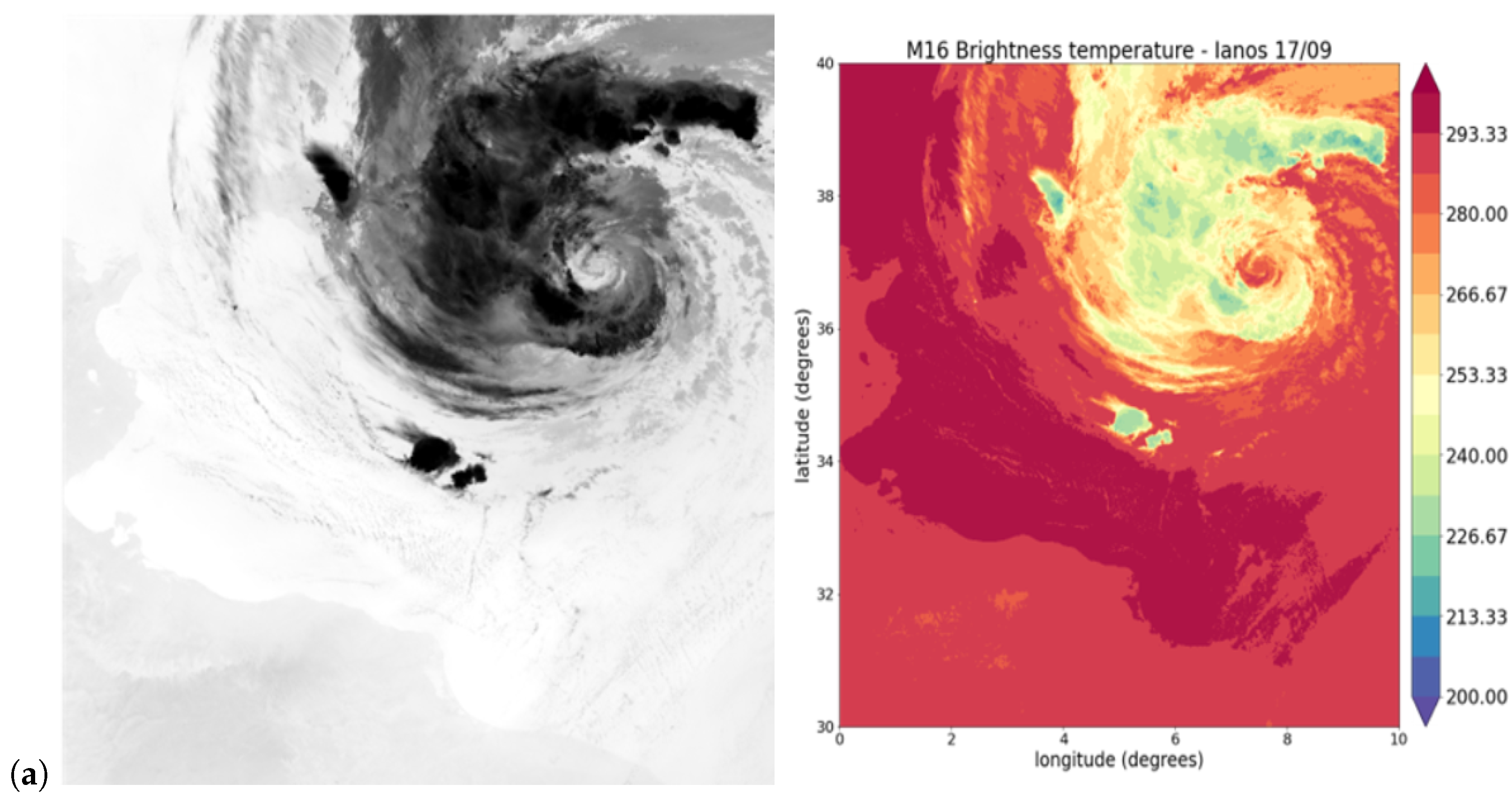
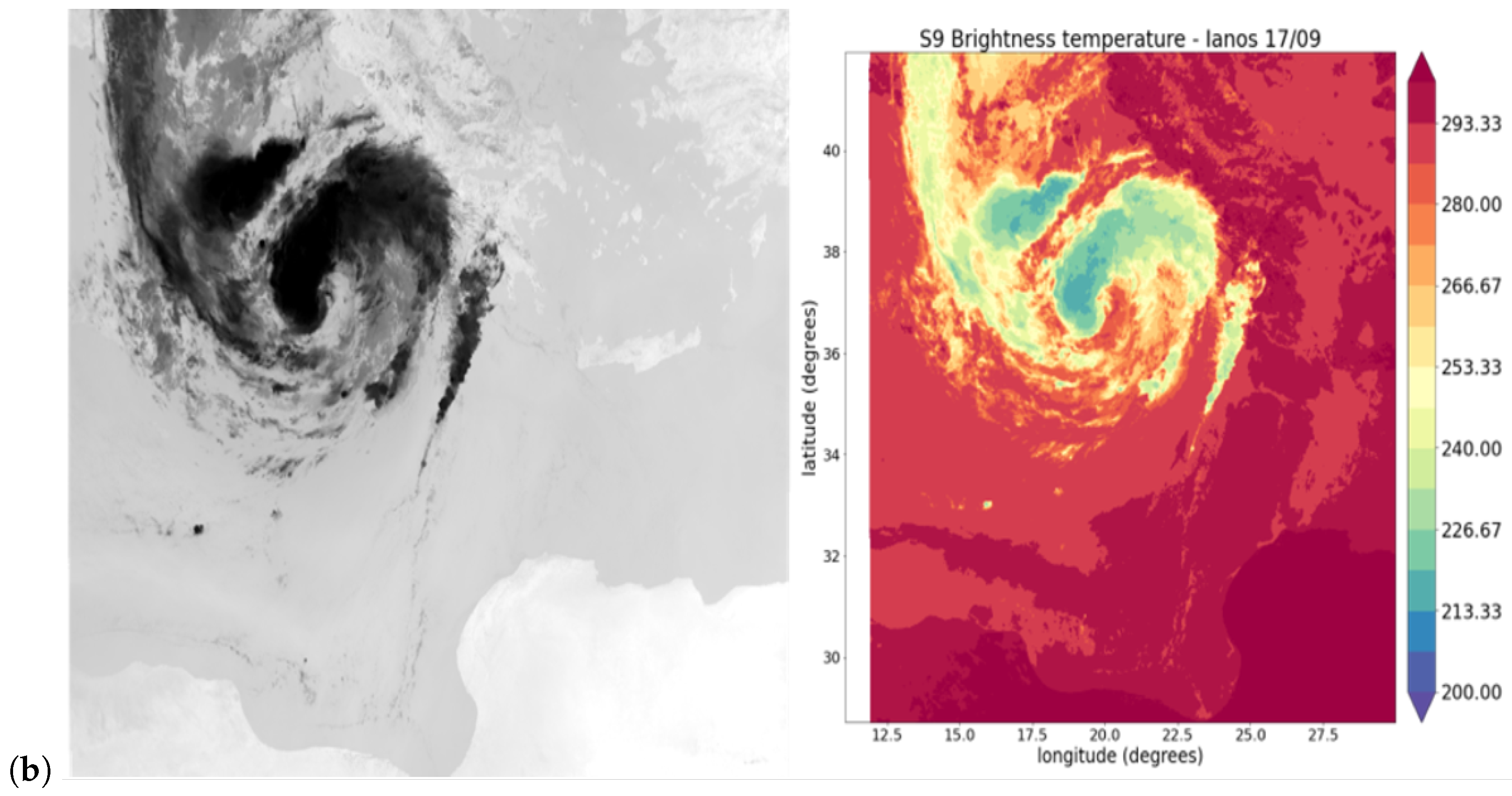
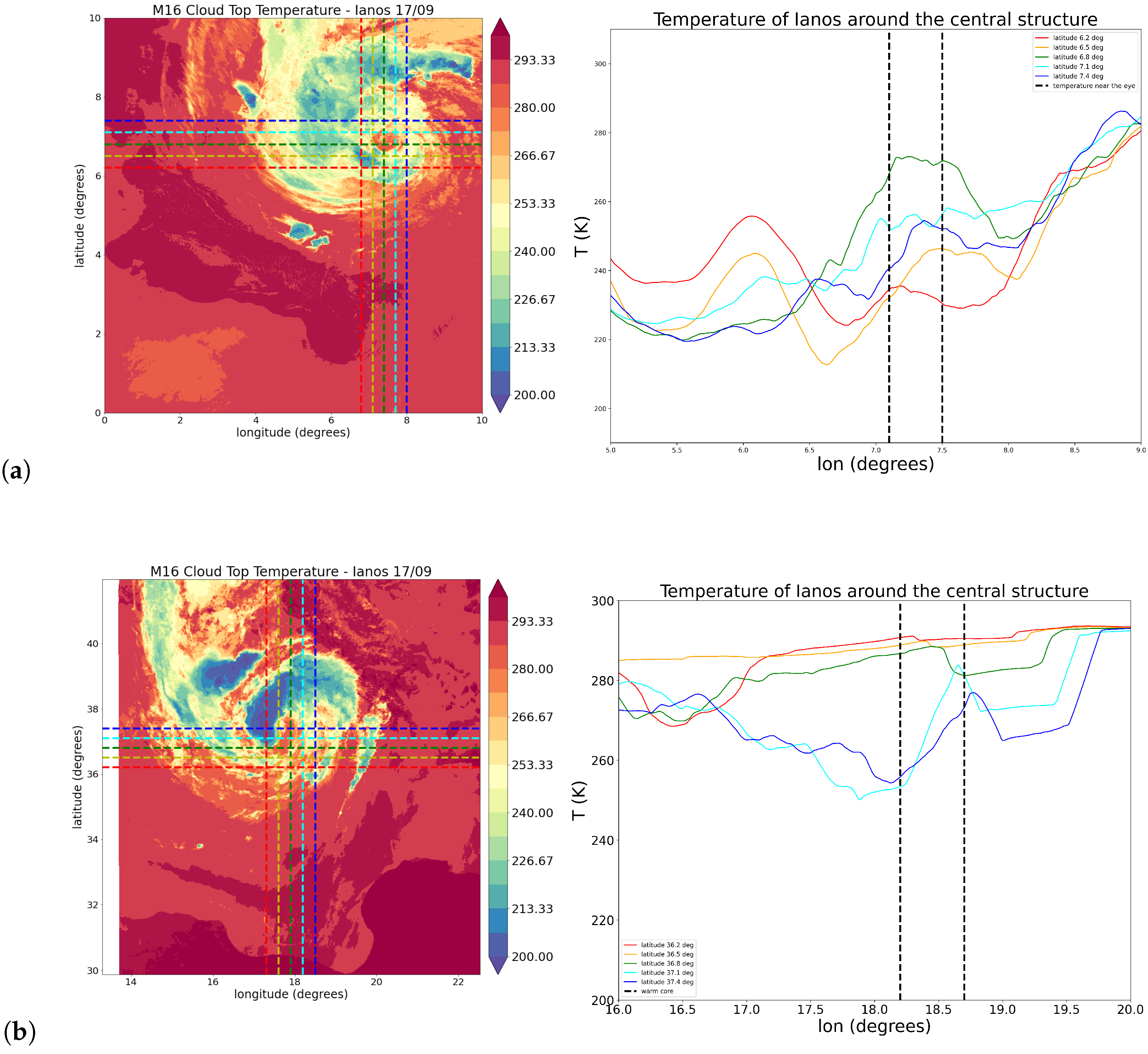
The evolution of Ianos and Apollo TLCs is monitored by exploiting brightness temperature for each sensing time. Starting from the radiation amount taken from the sensor, brightness temperature is used to extract other meaningful atmospheric fields, providing an improved assessment of the TLC cloud systems. Satellite observations are analyzed by deriving cloud top altitude and temperature, vertical temperature gradient, and atmospheric pressure field [23,24]. Altitude and temperature are obtained by considering drops in air temperature and the dew point in standard atmospheric conditions, while sea surface temperature is taken into account in the evaluation of the atmospheric instability through the vertical temperature gradient. The same standard conditions are leveraged to extract pressure from the images. Air temperature and sea surface temperature, in our procedure, involves the daily recorded data obtained as outputs from the BOLAM forecasting model [25,26]. From the same model, mean sea level pressure (MSLP) values are considered for comparison with values extracted for the pressure around the eye of the TLCs. The brightness temperature from two different spectral channels of VIIRS and SLSTR acquisition adds important information to describe the behavior of convection within the regions of the cyclonic structures, looking at the deep convection cloud pixels [27,28,29] and the ice percentage ones in the system.
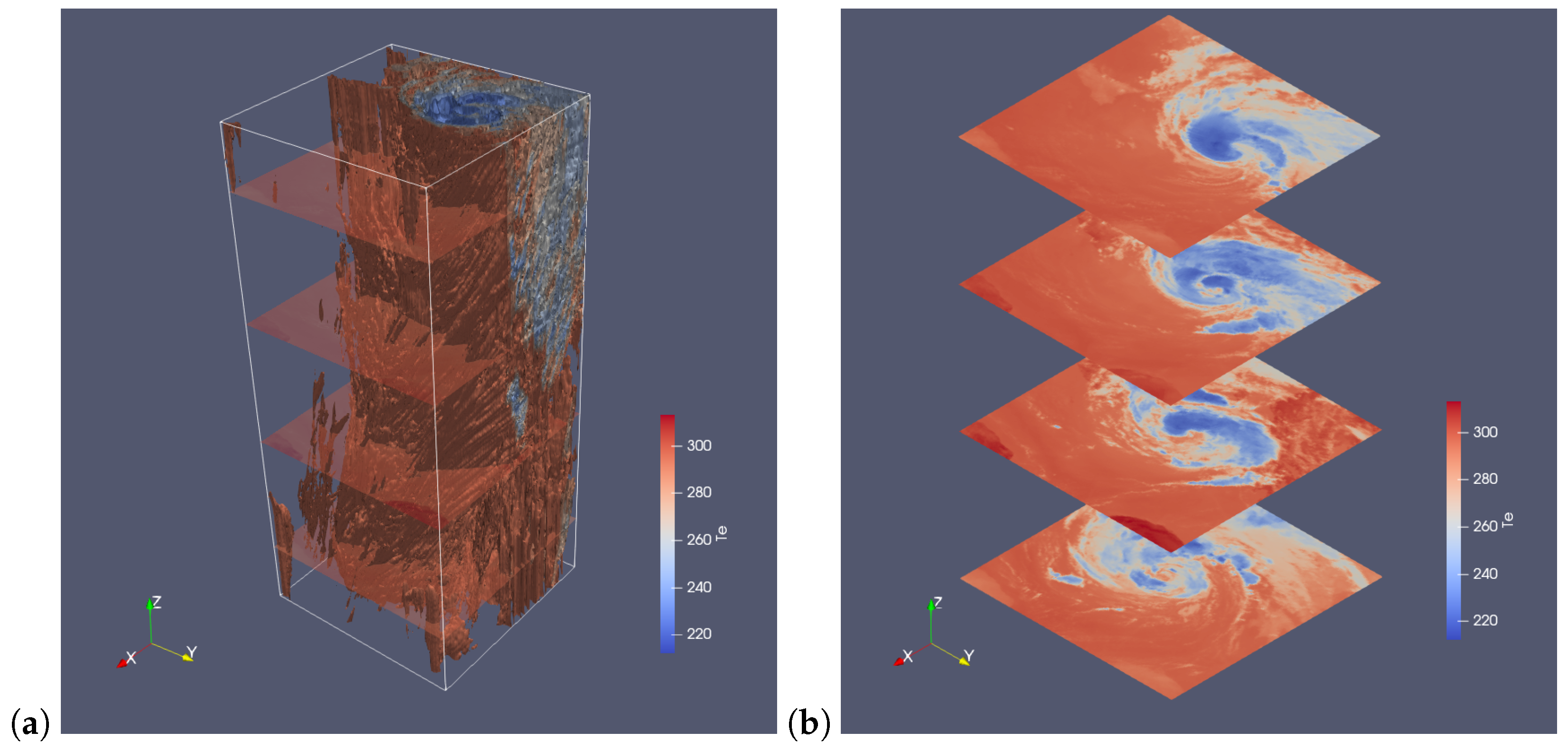
In the last part of the study, a 3D visualization is implemented by using ParaView software version 5.11.0 (https://www.paraview.org/ (accessed on 8 April 2024)) in order to investigate the evolution of Ianos. In this analysis, a database larger than the previous ones is exploited, acquiring the Ianos images by the spinning enhanced visible and infrared imager (SEVIRI) sensor, on the rapid scan high-rate service onboard Meteosat second generation-11 (MSG-11) satellite platform [30]. MSG-11 is a geostationary satellite platform and, if compared with LEO ones, it allows images and data with a lower spatial resolution (pixel size between 3 and 13 km) on a total globe coverage, with a very high temporal resolution (each image is obtained in a 5 min timestep in the rapid scan high-rate SEVIRI service). Moreover, 384 products are acquired, representing visualizations every 5 min one a one-day total period of Ianos’s evolution (on 17 September). In this database, the temperature field is contained in the pixels of the products, capturing all the timesteps of Ianos in the z-axis of the rearranged 3D view.
Ianos represents the most powerful cyclone observed in recent years in the Mediterranean basin [31]. It emerged from a cyclogenetic area connected to strong thunderstorms near the Gulf of Sidra, Libya, early on 15 September 2020. A rapid intensification occurred in the subsequent hours, reaching a very significant pressure minimum and a strong potential to acquire tropical features, powered by sea temperatures. Ianos gradually intensified over the Ionian Sea from late 16 September to early 17 September, acquiring the eye structure and Medicane features. The peak of intensity was reached near the Greek coasts in the first three hours of 18 September, when Ianos became equivalent to a second-category hurricane on the Saffir–Simpson scale. In the next two days, the structure started a weakening trend after making landfall in Greece, until it completely dissipated near the coast of eastern Libya.
Apollo, a little more than one year after Ianos, developed into a significantly strong Medicane with a wider track, encompassing two-thirds of the Mediterranean over a life period of about 10 days, between 25 October and 2 November 2021 [32]. Originating from a tropical disturbance in a thunderstorm area near the Balearic Islands, Apollo developed a low-pressure center in the first few days, intensifying and moving toward the Tyrrhenian Sea. The peak of intensity was reached on 29 October, after enduring strengthening off the coast of Sicily. Its convection slowed down for the first time on 30 October, and the dissipation trend ended a few days later, with residual strong winds pushing the system toward the Turkish coast.

2. Methods

The performances and capabilities of sensors onboard satellite platforms represent developing tools for observational approaches. With technological advancement, the potential of satellites is being fully exploited to monitor the increasing instability related to the effects of climate change on different global scenarios [33]. This study highlights a new perspective on diagnosing extreme events related to atmospheric mesoscale over the Mediterranean basin using a satellite remote sensing approach. As previously acknowledged for studying the diagnostics of a tropical cyclone at its maximum intensity category [23,24], a similar methodology is employed for comparing two Medicanes, aiming to seek atmospheric characterization from the medium-high resolution satellite data provided by two important LEO sensors. Their technical specifications for imagery acquisition are summarized in Table 1.
The choice of the satellites leads to a new analysis of the evolution of event dynamics, performed through the calculation of the atmospheric parameters of interest. For SLSTR, onboard the Sentinel-3A/B satellite missions, the descending sun-synchronous orbit crosses over the equator at 10:00 UTC, capturing the pixel with an oblique conical scanning in two different swaths of revisiting interval. On the other hand, VIIRS is characterized by an ascending sun-synchronous orbit, crossing over the equator around 13:25 UTC, with parallel lines pixel scanning.
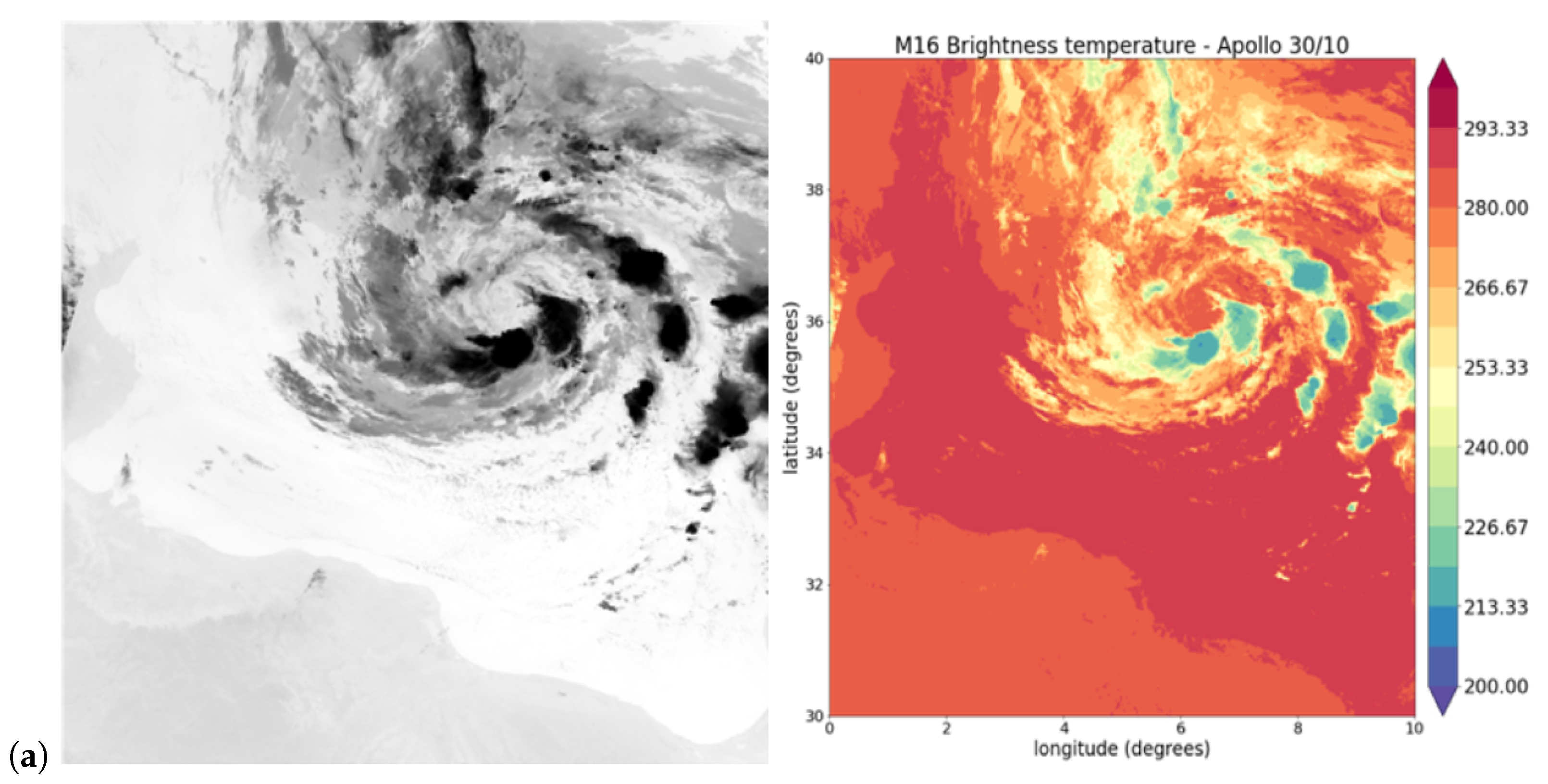
Imagery acquisition is specifically chosen to assess the two TLCs’ temporal evolution and their spatial displacement over Mediterranean latitudes with the best precision. Generally, according to Wien’s law, TIR spectral channels are the most appropriate to estimate the temperature of the Earth’s surface (LST—land surface temperature). At 27 °C (300 K), this parameter will have a wavelength peak emission at about 10 μ m, while wavelengths between 11 and 12 μ m and 15 μ m are more suitable for evaluating the cloud’s temperature and formation properties, up to 50 °C (220 K). Therefore, for this analysis, the TIR spectral channels of the two sensors are taken into account, which are identified with the resolution bands S8–S9 for SLSTR and M15–M16 for VIIRS. Central wavelengths for TIR1 bands (S8 and M15) are λ c = 10.76 μ m, while the ones for TIR2 bands (S9 and M16) are λ c = 12.01 μ m.
An initial check of the raw product marks the starting point of the analysis. In this pre-processing phase, the primary step involves optimizing the information in the pixels of each image. Different boundary conditions in the ( l o n , l a t ) grid visualization lead to the application of resizing and pixel resampling corrections. In particular, each image undergoes georeferencing [35], involving geographical correction to achieve uniform resized images through a nearest neighbor pixel resampling algorithm and a reprojection on the ellipsoid system UTM WGS-84.
After this first phase, the images are processed to compute the atmospheric parameters of the events. The grid of pixels in these newly resampled products contains data in brightness temperature, T b . Although this metric lacks direct physical significance, T b depends on the central wavelength (hence, the specific TIR spectral channel) and is proportional to the radiation amount recorded on the satellite sensor, L λ , at the moment of acquisition. For this reason, since the relationship is described by Planck’s law [36,37] (Equation (1)), T b denotes the thermal response of the total radiation recorded at the sensor, neglecting its reflection contribution along the object-satellite line of sight:
T b = h c ( k λ c ) 1 ln ( 2 h c 2 λ c 5 L λ + 1 ) .
where h = 6.626 × 10 34 J s is Planck’s constant, c = 3 × 10 8 m/s denotes the speed of light, and k = 1.38 × 10 23 J/K is Boltzmann’s constant.
T b data offer initial insights into the regions observed within the satellite imagery, depending on the wavelengths of both spectral channels. To enhance the observed scene, a temperature map is applied to each image, in which the total range of T b values is divided into 15 sub-ranges, assigning them different colors. This tool can help identify objects in the scene according to the range values, representing the first step of focusing on the cloud cluster characterizing the cyclone.
Following this initial step, the TIR2 resolution band of the two sensors is selected to derive the first two atmospheric parameters. We propose evaluating the scene by computing the altitude H from the top of the observed cloud system, and the associated temperature field T e f f . Their derivation is based on the coupling of two linear equations (Equation (2)), from which, values of H and T e f f are significant for the physical representation of the satellite view, particularly for the clouds associated with the cyclonic system:
T e f f = 0.00984 H + T a m b T e f f = 0.00182 H + T D
The calculation involves two constant numerical parameters, representing the conditions of air temperature drop (9.84 K per 1000 m of altitude, in K/m units) and dew point drop (1.82 K per 1000 m of altitude, in K/m units) [38]. These constants allow deriving a real temperature value, providing T a m b , given by the daily averaged output value of air temperature at 2 m above mean sea level (AMSL), acquired from the BOLAM forecasting model database. The overall calculation of H and T e f f must be completed by a generally known criterion used for assuming that the satellite-recorded T b values, under suitable instability conditions, can coincide with the dew, T D , at the altitudes of the condensation level [24]. With this procedure, by imposing T b = T D , system (2) is solved, and the quantities H and T e f f are obtained (Equation (3)).
H = ( T b T a m b ) ) / ( 0.00802 ) T e f f = 0.00984 [ ( T b T a m b ) ) / ( 0.00802 ) ] + T a m b
An evaluation of atmospheric instability conditions is carried out from the TLC computed values of H and T e f f . The investigation consists of computing the values of the vertical temperature gradient | T | by studying the relationship between the temperature’s positive variation in the layers of the cyclone and the altitude, expressed by Equation (4).
| T | = | T e f f T s s | H
In this equation, the quantity, T s s , represents the daily averaged sea surface temperature (higher than T e f f in all the scenes, except for the values associated with the sea surface area), obtained as outputs of the BOLAM forecasting model database, in order to obtain a local estimation of the temperature variation with the cloud stratification. Following this interpretation, the derived values can describe how the instability evolves with the daily Medicanes evolution if compared to the gradient limit values that—in an atmospheric general context—identify the degree of instability, as follows:
(1)
| T | > 0.01 K m−1 (absolute atmospheric instability), in which the numerical value is the dry adiabatic vertical gradient;
(2)
0.006 K m−1 < | T | < 0.01 K m−1 (conditional atmospheric instability), in which the vertical temperature gradient is included in the range’s moisture-to-dryness vertical gradients.
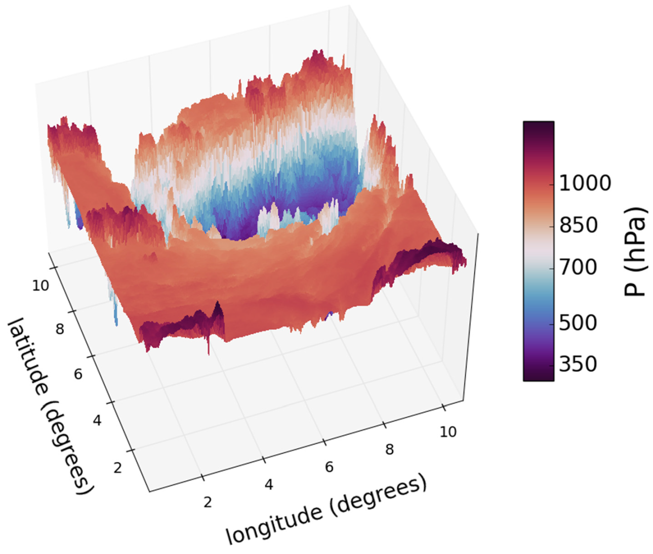
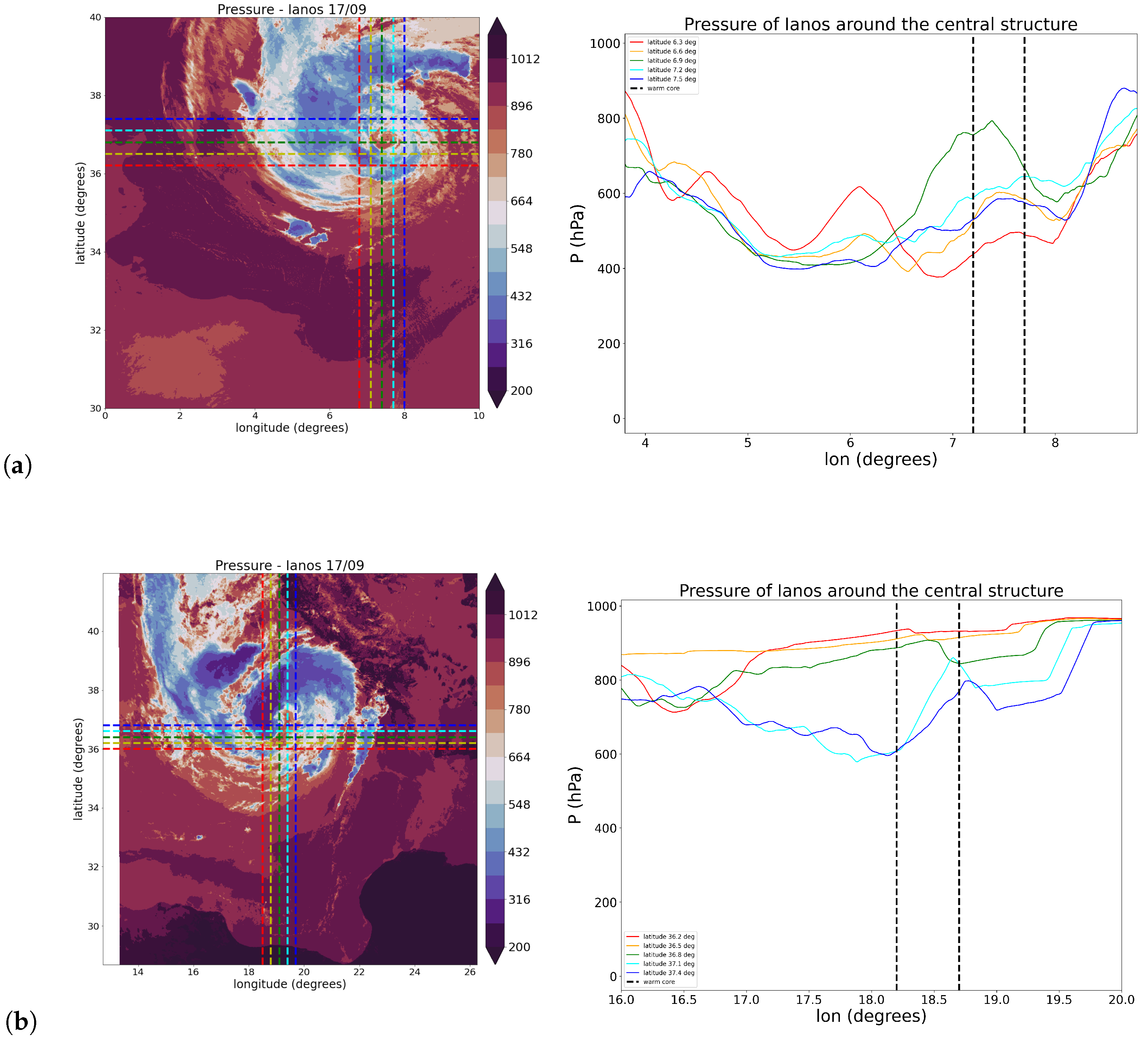
The next step entails calculating the atmospheric pressure field. In particular, considering the previously obtained altitude values alongside the standard atmospheric sea level pressure as P 0 = 1013.25 ± 1.00 hPa, the pressure field can be derived using the exponential law (Equation (5)).
P = P 0 e H / α
where
α = R D T ( H ) g
In Equation (6), α represents the scale height parameter, T the temperature, R D the specific gas constant in dry air, and g the gravitational acceleration. As the initial assessment to compute the pressure field, a constant value of the scale height equal to α = 8500 Km is selected, representing the typical air temperature under general standard conditions of the Earth’s atmosphere ( T = 290 K) [16,17]. This step is supplemented by examining the pressure field in the area surrounding the eye of the cyclone, on the peak intensity days of Ianos and Apollo, followed by a direct comparison with the MSLP output data recorded in the BOLAM databases.
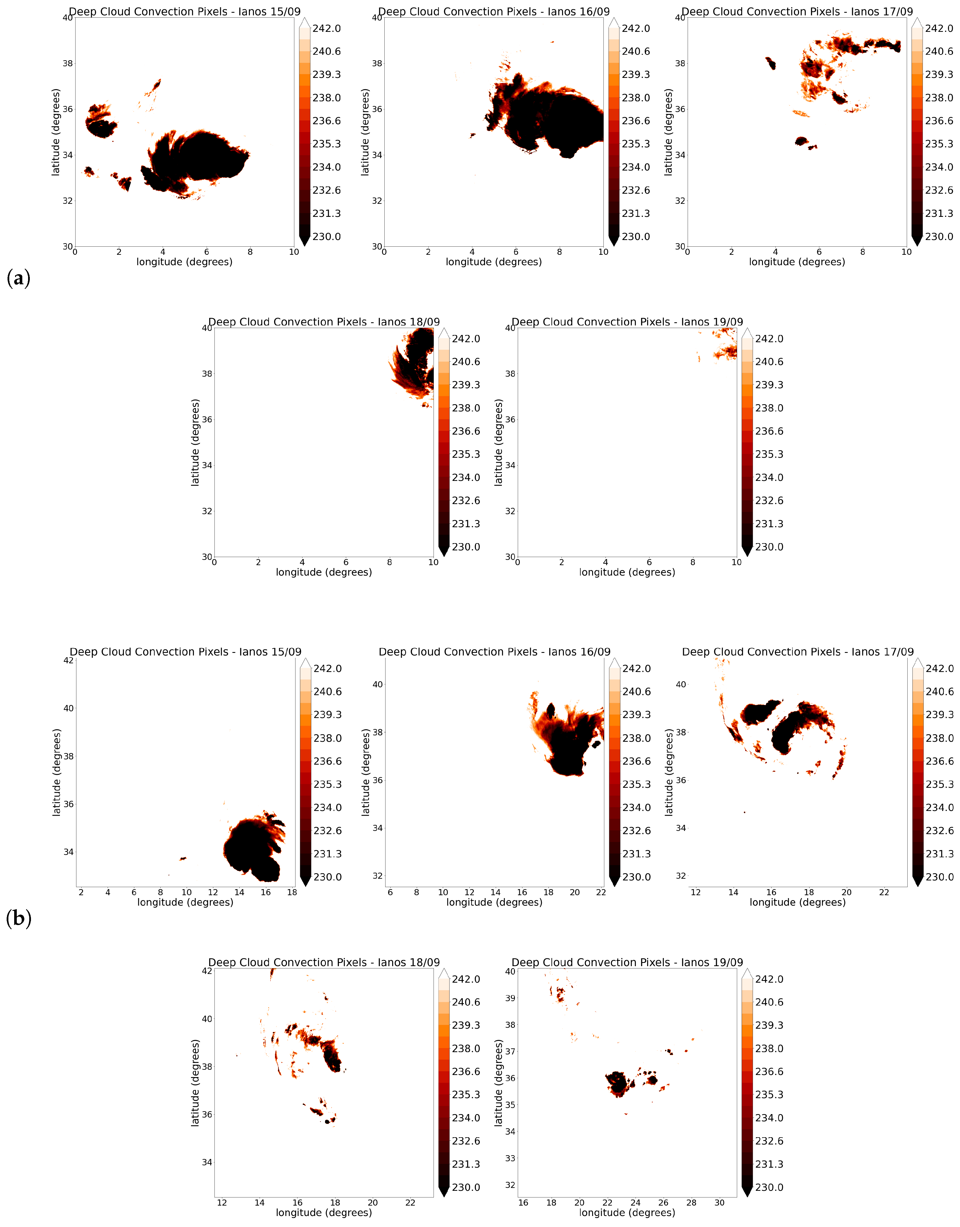
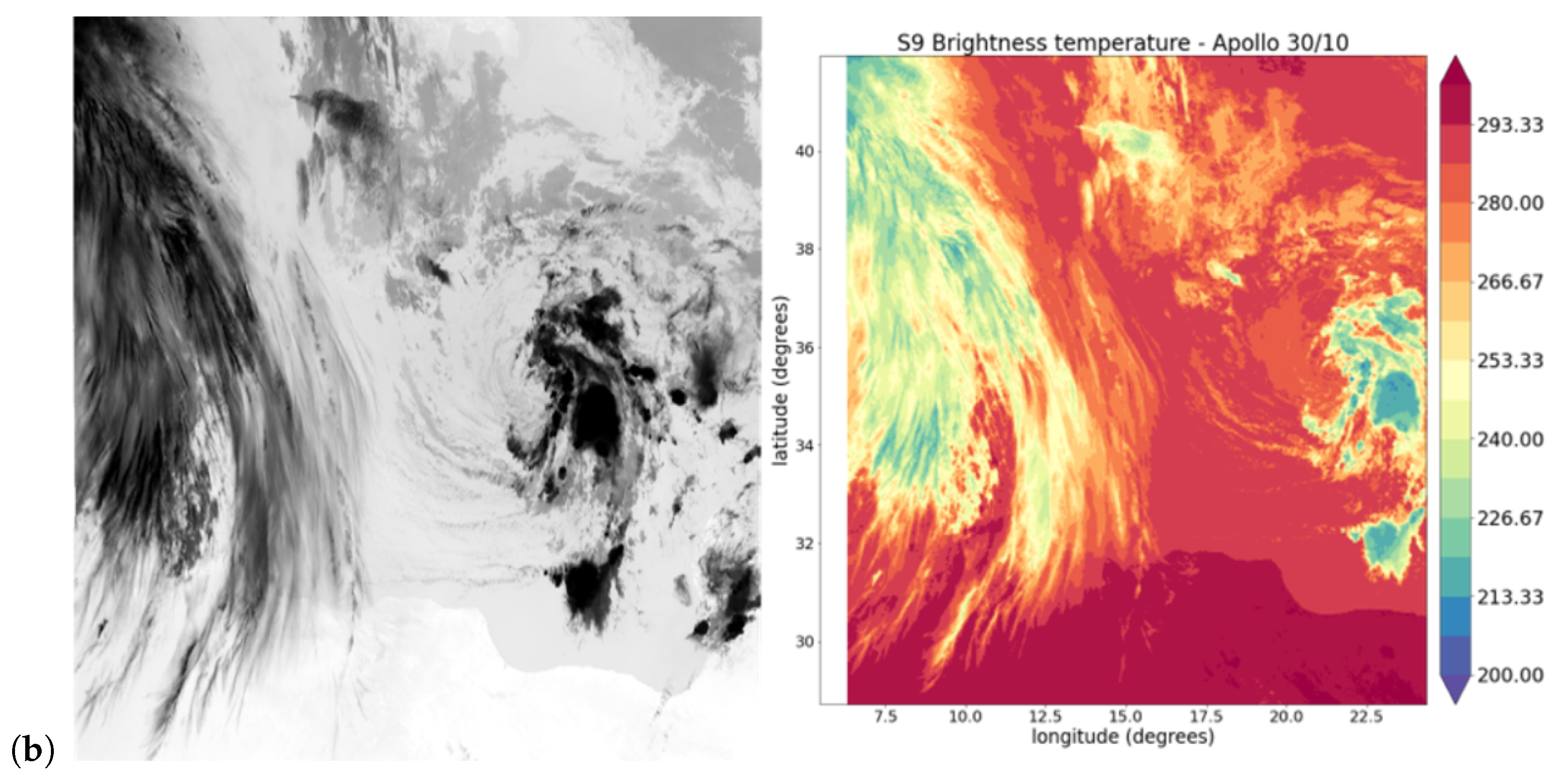
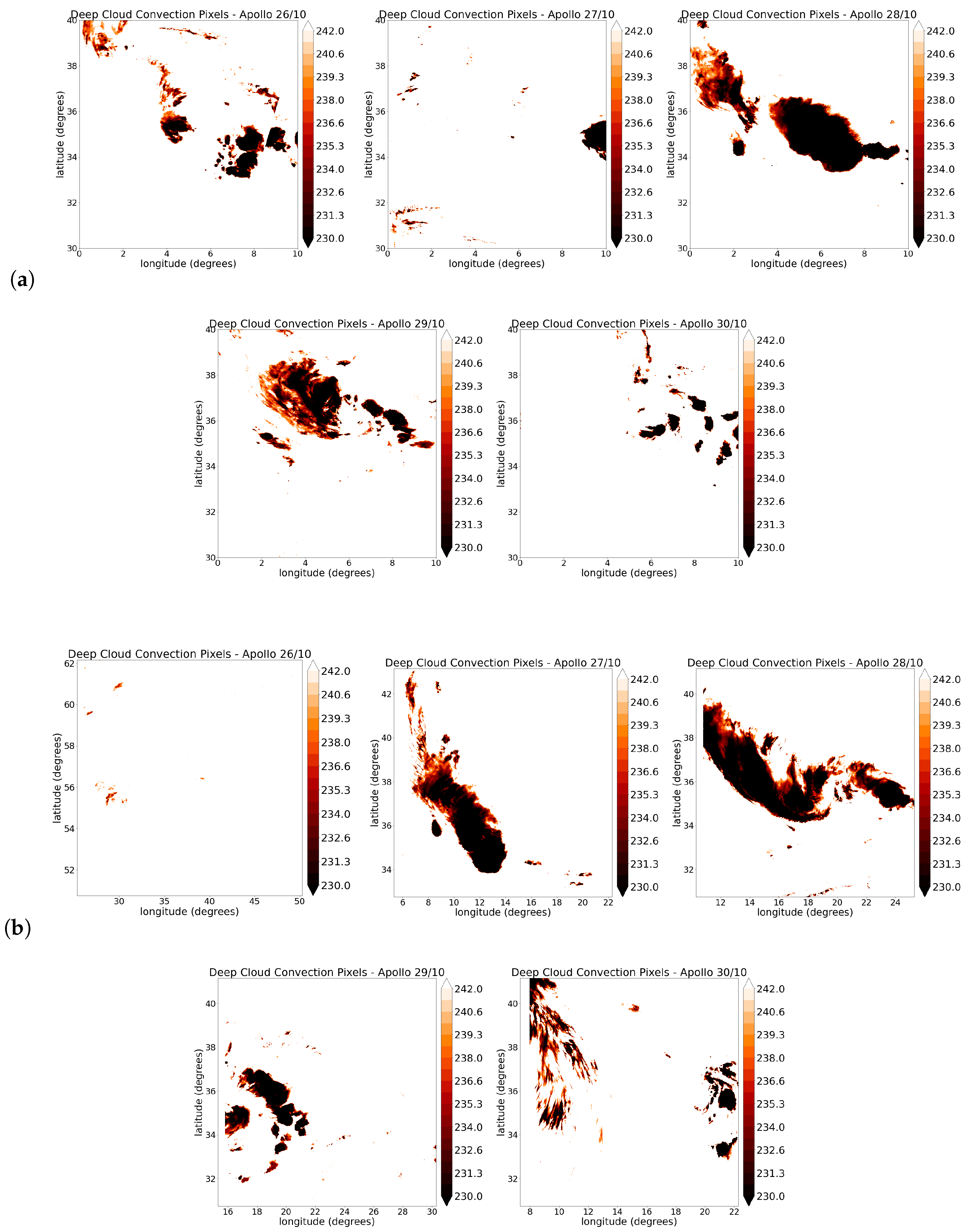
As mentioned above, several studies point out the important role of convection mechanisms in the process of cyclogenesis. One approach to identifying convection, as proposed by [27,28,29], involves the detection of pixels associated with deep convection clouds, in a direct way from the scene that highlights the different phases of the cyclone. Accordingly, we propose observing convection for the two Medicanes by exploiting the brightness temperature range, 230 K < T b < 240 K, of the georeferenced images displayed in the TIR1 spectral channel.
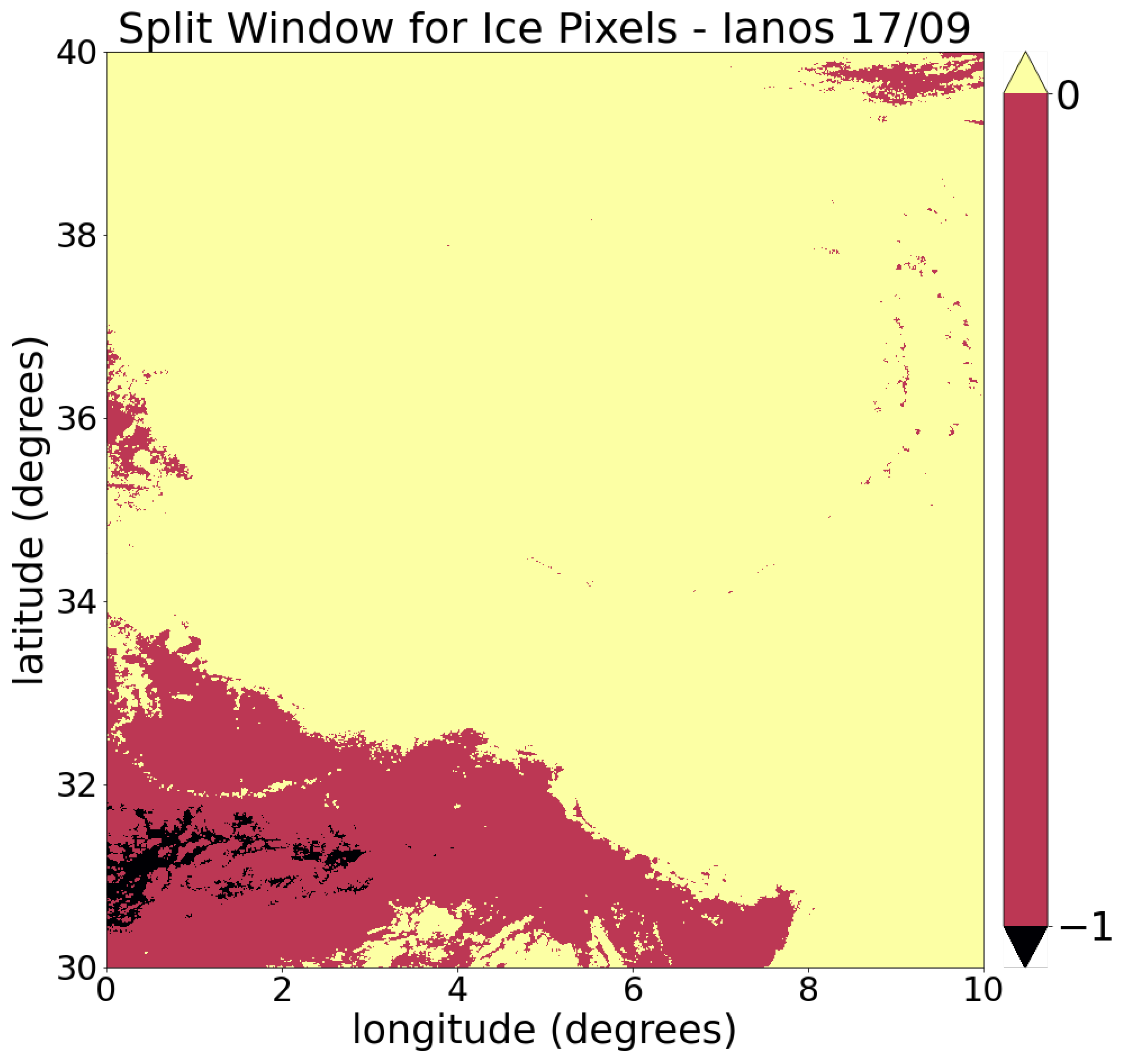
To validate the presence of strongly convective clouds in the structure of the Medicanes, the split window spectral method is applied [39], which is generally associated with cirrus cloud detection in the system, and is hereby proposed to search for the ice percentage pixels in the cloud layers of the cyclone:
Δ T = T b ( T I R 1 ) T b ( T I R 2 )
The method is based on the difference in brightness temperature values of both spectral channels of the TIR, as expressed in Equation (7). Each image is the result of subtracting the two TIR views of the same scene, where the values within the range of 1 K < Δ T < 0 K identify the pixels of ice in the clouds.
By exploiting some technical features of the ParaView software, it is possible to obtain a 3D visualization of the temporal evolution of Ianos, precisely by considering time as the third vertical dimension, together with the two horizontal dimensions provided by the longitude and latitude in the SEVIRI images. The database products are characterized by a 5-minute timestep over a one-day total period of the cyclone’s life, with a spatial pixel size of 4 km. Each image is the result of a pre-processing step that allows locating the cyclone in its impact area, representing the temperature field (extracted by solving Equation (3)) in the TIR spectral channel of SEVIRI (central wavelength λ c = 10.8 μ m).

3. Results

In this section, the previously explained analysis procedure is applied to the Ianos and Apollo TLCs in two different subsections, before arranging the final comparison of their atmospheric parameters of interest.

3.1. Ianos Analysis

Ianos scenes reprojected from VIIRS TIR products consist of a geographical grid equal to Δ R = N l o n × N l a t = 2400 × 2400 pixels, where N l o n and N l a t identify the longitude pixel number and latitude pixel number, respectively.
SLSTR products do not visualize the same scene at all sensing times, but each image consists of a reprojected view of Δ R = N l o n × N l a t = 1200 × 1200 pixels. The SLSTR spatial coordinates are provided by the raw data and reprojected on the same system. They vary, depending on the sensing daytime of the images and, thus, on the choices made to best visualize the evolution of the large-scale Ianos central structure over the different life days. The full dataset is presented in Table 2.
It is worth noting that images acquired in daylight sensing times (three from the SLSTR sensor) are affected by reflected radiance. The presence of this quantity changes very little in the visualization of images in TIR bands and may contribute to a slight overestimate of the temperatures. Hence, asterisks near the night hours are marked in the table. It should be noted that the VIIRS products are acquired and reprojected according to the pre-processing on the same 2D geographical grid for all the days of the evolution of Ianos, in order to obtain useful information on the cyclone’s impact area.
The pre-processing phase for Ianos products is presented in panels (a,b) of Figure 1, where the raw images are shown on the left, and the results of the same images, after the resampling and reprojection processes, are displayed on the right side of the figure as temperature maps of the quantity T b .
Using this first representation, it is possible to calculate the values of H and T e f f by taking into account the BOLAM recorded data of daily temperature at 2 m AMSL. The first column in Table 3 presents this parameter extracted for Ianos life days. Once the T e f f representative map is obtained, it is possible to identify information about the physics of the system from a direct comparison with the T b initial map, as shown in the panels of Figure 2. Very significant differences in the temperature values, particularly inside the rotating clouds around the warm core of Ianos (in that specific life day), are highlighted when comparing brightness temperatures (panels a,c) with cloud-top ones (panels b,d), for both satellite databases.
Starting with temperature, and aimed at providing a semi-qualitative assessment of the presence of strong atmospheric TLC instability, the vertical temperature gradient, | T | , is derived using Equation (4), and recorded T S S values contained in the second column of Table 3. In Figure 3, (a) and (b) panels, it is observed that, everywhere in the cloud regions associated with the cyclone, the gradient values identify absolute instability throughout Ianos life days ( | T | > 0.01 K m−1 for the cyclone in all the scenes). The white colors in the maps mark the areas on or near the surface (where H values tend to be zero and the temperature differences are very small). The black color represents a mask attributed to the radiometric effects over the Earth’s surface pixels from the SLSTR database. It is associated with values very close to | T | 0 K m−1, in which land surface temperature and cloud-top are mostly coincident.
Further comparisons for Ianos datasets are extracted from the temporal trend of the atmospheric pressure field, calculated with the exponential law in Equation (5). From the results, a detailed analysis of the pressure values is consistent with a non-flattened view of the scene, which provides significant information on the stratification of the cloud system in the different zones defining the Ianos central structure. Following the reference outputs of T a m b and T S S , an observation for detecting the temperature variation in the inner central part of the cyclones is shown in Figure 4. The comparison between VIIRS and SLSTR is shown for the two spatial trends of the cloud top temperature of Ianos as a function of longitude, by setting different latitude values around the central area. It provides a qualitative assessment of the warm core detection on the day of maximum intensification. The warm core presence, observed from the top of the cloud, on this day of Ianos evolution, is enhanced in Figure 5 by the pressure field spatial trends, with the focus on the values around the eyewall identification. A characterization of the maximum value of MSLP, extracted from VIIRS and SLSTR products, leads to an estimation of the pressure in the eye of the cyclone through daily comparison with the recorded MSLP data; values are presented in Table 4.
The last two significant investigations for Ianos include a specific study of the clouds of the system. By exploiting the images in both TIR spectral channels, identifying the convective and the ice clouds is possible. In particular, the use of the TIR1 spectral channel, displaying T b data, can help to trace the deep convection in the scene, as proposed by [27,28], in the brightness temperature range containing the values between 230 K and 240 K. In Figure 6, we report the daily evolution representation in which the deep cloud convection pixels (DCCPs) inside the Ianos organizing structure (panels a,b for VIIRS and SLSTR, respectively) are highlighted. Moreover, in Figure 7, an example of the VIIRS image for the Ianos ice percentage pixels is included after the application of the split window technique. In this visualization, the ice percentage is almost entirely absent, and the colored values in the bottom part of the view represent the temperature differences associated with the land area. The SLSTR example of this characterization is not shown because of the absence of appreciable variations compared with the VIIRS one.
To characterize and conclude the Ianos analysis, a 3D observation of the evolution of the cyclonic structure in time and space is shown in Figure 8. Panel (a) of this figure denotes the contour volume (obtained with the software ParaView), in which all the SEVIRI products of Ianos are inserted by considering a grid of Δ R = N l o n × N l a t = 350 × 350 pixels in the (x,y) plane, evolving in one day, with 5 min timesteps, over the z-axis. This contour volume is obtained with eight different sub-ranges of the total temperature range of the images, from T m i n = 212 K to T m a x = 292 K, with a width of Δ T = 10 K. In panel (b), four of all the products are shown as slices of the total volume (made opaque in the left panel), showing four specific timesteps of the Ianos intensification during the chosen life day. With this new observational perspective, a detailed study of the shape and direction of the different layers of the cyclone’s main cloud system was carried out. The main focus was on changes over very short timesteps and in the specific geographical area of its impact. This involved selecting both the moments of interest and the temperature values associated with different spatial zones, from the outermost cyclonic regions to the eyewall.

3.2. Apollo Analysis

The analysis of Apollo TLC was carried out over a period of five days between 26 and 30 October 2021, highlighting the formation and intensification of main moments. The list of exploited VIIRS and SLSTR images is shown in Table 5. The same pre-processing phase of resampling and reprojection is applied over the geographical ( l o n , l a t ) grid, as displayed in panels (a,b) in Figure 9.
All the procedures for extracting atmospheric parameters follow the same workflow used for Ianos. Values of H and T e f f are calculated by performing the temperature maps and using the daily average temperature at 2 m a.s.l. values recorded from BOLAM (reported in the first column of Table 6).
Detailed analyses of the cyclonic structure are shown in Figure 10, with the vertical temperature gradient assessment. Although it is once again possible to identify the presence of absolute instability for Apollo, its shape related to unstable clouds seems to be not well defined in some product views. Taking this into account, in the study of atmospheric pressure data from the images, we opted for assessing the pressure minimum in a larger area, tracing back to an area closest to the warm core of the system. The values of the low-pressure center extracted for all Apollo sensing times are reported in Table 7 and compared once again with the BOLAM MSLP recorded data.
Again, for Apollo, identifying deep convective clouds and ice clouds is performed according to the same techniques used for Ianos. The DCCP result representations for the cyclone are shown in Figure 11, where the contribution of convection helps to better understand the dynamics of the rotating air mass during cyclogenesis, despite the fact that the cyclonic structure is hardly distinguishable in some of its life days.

4. Discussion and Conclusions

Satellite remote sensing tools represent fundamental resources for scientific research on the characterization of a cyclonic system in Mediterranean latitudes, facilitating a detailed investigation of such complex meteorological events. Satellite-collected data facilitate the study of Mediterranean cyclone formation and development, particularly by observing clouds, air currents, and thermal variations with advanced space-based instruments.
Satellite payloads, providing information in TIR spectral bands, enable studying these kinds of events on different life days through the characterization of their cloud systems, with a focus on stratification and rotating air mass circulation. Atmospheric parameter derivation primarily relies on radiance-at-satellite responses, providing insights into upper cloud layer atmospheric conditions.
LEO platforms, such as Suomi NPP and Sentinel-3, in addition to the GEO MSG-11, yield data about the brightness temperature field in the TIR spectral channels, by observing large and intermediate scales of cyclones from the top of the cloud [23].
Daily T a m b and T S S data recorded by the BOLAM forecasting model allow for the assessment of the vertical thermal gradient, highlighting the central large local stratification in different regions, and its correlation with the instability degree for both Medicanes examined in this work.
BOLAM-recorded data are also useful in analyzing the atmospheric pressure field extracted from the images. A comparison with the daily MSLP shows consistency with the satellite-extracted pressure values, identifying the area of the cyclonic warm core in both cases. The derivation of pressure values in the eye area (or in the surrounding areas of the warm core) is consolidated by studying the daily spatial trend of the pressure, even if not all associated graphs are shown. However, it can be seen that the pressure field obtained from VIIRS data appears to be slightly closer than SLSTR, with respect to those recorded. For Apollo Medicane, estimates of MSLP that were obtained from BOLAM, VIIRS, and SLSTR can be compared with the results obtained by Menna et al. [40]. Comparing their Figure 2 (panels b,c), the values extrapolated from the plots, from 26 October to 30 October, yield results absolutely similar to ours reported in Table 7, particularly in the measure trends and the absolute values, with relative differences, ∼1 %.
As in the analysis for the case study of a tropical cyclone [24], the high-quality scanning technique operated by VIIRS, combined with daily nighttime acquisition at 00:00 UTC, enhances accuracy in the results by minimizing reflected radiance effects.
Additionally, the fusion of TIR spectral channels from multiple sensors can help to identify the image pixels associated with the clouds responsible for deep convection. By replicating the procedure previously used in [27,28,29], it can be seen that convection evolves in most cases within the clouds rotating around the central structure of the inner core. This helps provide a qualitative contribution to understand the dynamics of the two cyclones. Furthermore, using the split window technique, the absence of ice percentage pixels associated with the cloud systems on the TLCs’ life days is revealed. Future efforts will involve exploring new satellite data sources and potential combinations with operational PMW sounders to refine parameter extraction for mapping Medicanes from the inner part, as suggested in [20]. Further improvements in the efficiency of this type of study can be achieved by comparing and combining data from observations with data obtained from numerical simulations, reanalysis models, or the acquisition of ground-based measurements.
Our aim is to delve into high-quality data obtained from cutting-edge satellite platforms, encompassing their polar low orbits. Specifically, we consider measuring and understanding the impact of relative humidity and wind speeds within the cyclone system [41], with an important focus on the several phases of its life period. By incorporating these variables, our analysis would provide a more comprehensive perspective on the intricate dynamics. Nevertheless, this type of analysis applied to TLC evolution is also a key point for us, with significant ongoing investigations about the role of convection and moist static energy in the cyclogenesis processes [14,15], leading up to the formation of the warm inner core.
The integration of several satellite data sources contributes to a holistic approach, paving the way for more effective strategies in predicting, managing, and responding to extreme meteorological events.

Author Contributions

Conceptualization, V.C. and F.F.; methodology, G.C., L.P. and F.F.; software, G.C. and L.P.; validation, V.C., F.F. and F.L.; formal analysis, G.C. and L.P.; investigation, G.C.; resources, G.C. and F.F.; data curation, G.C. and F.F.; writing—original draft preparation, G.C. and L.P.; writing—review and editing, F.F. and F.L.; visualization, G.C.; supervision, L.P. and F.L.; project administration, F.F. and V.C. All authors have read and agreed to the published version of the manuscript.

Funding

G.C. is supported by the Italian “Ministero dell’Università e della Ricerca” (MUR) under the program PON “Ricerca e Innovazione” 2014–2020, Azione IV.5 — “Dottorati su tematiche green” tematica “Cambiamento climatico e accelerazione di eventi estremi nel bacino del Mediterraneo”.

Institutional Review Board Statement

Not applicable.

Informed Consent Statement

Not applicable.

Data Availability Statement

Data elaborated on in the present article were downloaded from the following site (accessed on 14 December 2023): https://view.eumetsat.int/productviewer?v=default, by selecting “Meteosat-11” for “Satellite”, “Rapid Scan High Rate SEVIRI IR10.8” for “Channels”; https://ladsweb.modaps.eosdis.nasa.gov (accessed on 14 December 2023), by selecting “VIIRS Suomi NPP”-“SLSTR ESA Copernicus Sentinel-3A”-“SLSTR ESA Copernicus Sentinel-3” for “Sensors”, -“VNP41A1”-“S3ASL1RBT”-“S3BSL1RBT” for “Products”.

Conflicts of Interest

The authors declare no conflicts of interest.

Abbreviations

The following abbreviations are used in this manuscript:
TLCtropical-like cyclone
LEOlow-Earth orbit
TIRthermal infrared
VIIRSvisible/infrared imager radiometer suite
SLSTRsea and land surface temperature radiometer
Suomi NPPSuomi National Polar-orbiting Partnership
SEVIRIspinning enhanced visible and infrared imager
PMWpassive microwave
LSTland surface temperature
MSLPmean sea level pressure
AMSLabove mean sea level

References

  1. Mazza, E.; Ulbrich, U.; Klein, R. The tropical transition of the October 1996 medicane in the western Mediterranean Sea: A warm seclusion event. Mon. Rea. Rev. 2017, 145, 2575–2595. [Google Scholar] [CrossRef]
  2. Fita, L.; Flaounas, E. Medicanes as subtropical cyclones: The December 2005 case from the perspective of surface pressure tendency diagnostics and atmospheric water budget. Quart. J. Roy. Meteor. Soc. 2018, 144, 1028–1044. [Google Scholar] [CrossRef]
  3. Emanuel, K.A. An air-sea interaction theory for tropical cyclones. PArt I: Steady-state maintenance. J. Atmos. Sci. 1986, 43, 585–604. [Google Scholar] [CrossRef]
  4. Lagouvardos, K.; Kotroni, V.; Nickovic, S.; Jovic, D.; Kallos, G.; Tremback, C.J. Observations and model simulations of a winter sub-synoptic vortex over the central Mediterranean. Meteor. Appl. 1999, 6, 371–383. [Google Scholar] [CrossRef]
  5. Miglietta, M.M. Mediterranean tropical-like cyclones (medicanes). Atmosph. 2019, 10, 206. [Google Scholar] [CrossRef]
  6. Miglietta, M.M.; Rotunno, R. Development mechanisms for Mediterranean tropical-like cyclones (medicanes). Quart. J. Roy. Meteor. Soc. 2019, 145, 1444–1460. [Google Scholar] [CrossRef]
  7. Davis, C.A.; Bosart, L.F. Baroclinically Induced Tropical Cyclogenesis. Mon. Weather Rev. 2003, 131, 2730–2747. [Google Scholar] [CrossRef]
  8. Moscatello, A.; Miglietta, M.M.; Rotunno, R. Numerical Analysis of a Mediterranean “Hurricane” over Southeastern Italy. Mon. Weather Rev. 2008, 136, 4373–4397. [Google Scholar] [CrossRef]
  9. McTaggart-Cowan, R.; Galarneau, T.J.; Bosart, L.F.; Milbr, J.A. Development and Tropical Transition of an Alpine Lee Cyclone. Part I: Case Analysis and Evaluation of Numerical Guidance. Mon. Weather Rev. 2010, 138, 2281–2307. [Google Scholar] [CrossRef]
  10. Fita, L.; Romero, R.; Ramis, C. Intercomparison of Intense Cyclogenesis Events over the Mediterranean Basin Based on Baroclinic and Diabatic Influences. Adv. Geosci. 2006, 7, 333–342. [Google Scholar] [CrossRef]
  11. Prat, A.C.; Federico, S.; Torcasio, R.C.; D’Adderio, L.P.; Dietrich, S.; Panegrossi, G. Evaluation of the Sensitivity of Medicane Ianos to Model Microphysics and Initial Conditions Using Satellite Measurements. Remote Sens. 2021, 13, 4984. [Google Scholar] [CrossRef]
  12. Miglietta, M.M.; Cerrai, D.; Laviola, S.; Cattani, E.; Levizzani, V. Potential Vorticity Patterns in Mediterranean “Hurricanes”. Geophys. Res. Lett. 2017, 44, 2537–2545. [Google Scholar] [CrossRef]
  13. Emanuel, K. Genesis and maintenance of “Mediterranean hurricanes”. Adv. Geosci. 2005, 2, 217–220. [Google Scholar] [CrossRef]
  14. Khairoutdinov, M.; Emanuel, K. Rotating radiative-convective equilibrium simulated by a cloud-resolving model. J. Adv. Model. Earth Syst. 2013, 5, 816–825. [Google Scholar] [CrossRef]
  15. Muller, C.J.; Bony, S. What favors convective aggregation and why? Geophys. Res. Lett. 2015, 42, 5626–5634. [Google Scholar] [CrossRef]
  16. Salby, M.L. Fundamental of Atmoshperic Physics; Academic Press: London, UK, 1996. [Google Scholar]
  17. Ahrens, C.D. Meteorology Today: An Introduction to Weather, Climate and the Environvment, 9th ed.; Brooks/Cole, CengageLearning: Boston, MA, USA, 2009. [Google Scholar]
  18. Wieczorek, A. Medicanes—The hurricanes of Mediterranean? Wetterdienst Thema Des Tages 2015, 1, 1. [Google Scholar]
  19. Hatzaki, M.; Flaounas, E.; Davolio, S.; Pantillon, F.; Patlakas, P.; Raveh-Rubin, S.; Hochman, A.; Kushta, J.; Khodayar, S.; Dafis, S.; et al. MedCyclones: Working Together toward Understanding Mediterranean Cyclones. Bull. Am. Meteorol. Soc. 2023, 104, E480–E487. [Google Scholar] [CrossRef]
  20. Panegrossi, G.; D’Adderio, L.P.; Dafis, S.; Rysman, J.-F.; Casella, D.; Dietrich, S.; Sanò, P. Warm Core and Deep Convection in Medicanes: A PAssive Microwave-Based Investigation. Remote Sens. 2023, 15, 2838. [Google Scholar] [CrossRef]
  21. Roman, M.O.; Wang, Z.; Sun, Q.; Kalb, V.; Miller, S.D.; Molthan, A.; Schultz, L.; Bell, J.; Stokes, E.C.; Pandey, B.; et al. NASA’s Black Marble nighttime lights product suite. Remote Sens. Environ. 2018, 210, 113–143. [Google Scholar] [CrossRef]
  22. Donlon, C.; Berruti, B.; Buongiorno, A.; Ferreira, M.-H.; Féménias, P.; Frerick, J.; Goryl, P.; Klein, U.; Laur, H.; Mavrocordatos, C.; et al. The Global Monitoring for Environment and Security (GMES) Sentinel-3 mission. Remote Sens. Environ. 2012, 120, 37–57. [Google Scholar] [CrossRef]
  23. Ciardullo, G.; Primavera, L.; Ferrucci, F.; Carbone, V.; Lepreti, F. Study of Turbulence Associated with the Faraji Cyclone. Climate 2022, 10, 21. [Google Scholar] [CrossRef]
  24. Ciardullo, G.; Primavera, L.; Ferrucci, F.; Lepreti, F.; Carbone, V. New Investigation of a Tropical Cyclone: Observational and turbulence analysis for the Faraji Hurricane. Remote Sens. 2023, 15, 1383. [Google Scholar] [CrossRef]
  25. Buzzi, A.; Fantini, M.; Malguzzi, P.; Nerozzi, F. Validation of a limited area model in cases of Mediterranean cyclogenesis: Surface fields and precipitation scores. Meteorol. Atmos. Phys. 1994, 53, 137–153. [Google Scholar] [CrossRef]
  26. Orlandi, E.; Fierli, F.; Davolio, S.; Buzzi, A.; Drofa, O. A nudging scheme to assimilate satellite birghtness temperature in meteorological model: Impact on representation of African mesoscale convective systems. Quart. J. R. Meteor. Soc. 2010, 136, 462–474. [Google Scholar] [CrossRef]
  27. Hong, G.; Heygster, G.; Rodriguez, C.A.M. Effect of cirrus clouds on the diurnal cycle of tropical deep convective clouds. J. Geophys. Res. 2006, 111, D06209. [Google Scholar] [CrossRef]
  28. Wu, Q.; Ruan, Z. Diurnal variations of the areas and temperatures in tropical cyclone clouds. Quart. J. R. Meteor. Soc. 2016, 142, 2788–2796. [Google Scholar] [CrossRef]
  29. Dafis, S.; Claud, C.; Kotroni, V.; Lagouvardos, K.; Rysman, J. Insights into the convective evolution of Mediterranean tropical-like cyclones. Quart J. R. Meteor. Soc. 2020, 146, 4147–4169. [Google Scholar] [CrossRef]
  30. Cao, C.; Xiong, X.; Wolfe, R.; DeLuccia, F.; Liu, Q.; Blonski, S.; Lin, G.; Nishihama, M.; Pogorzala, D.; Oudrari, H.; et al. Visible Infrared Imaging Radiometer Suite (VIIRS) Sensor Data Record (SDR) User’s Guide, version 1.2.; National Oceanic and Atmospheric Administration: Washington, DC, USA, 2013. [Google Scholar]
  31. Lagouvardos, K.; Karagiannidis, A.; Dafis, S.; Kalimeris, A.; Kotroni, V. Ianos—A Hurricane in the Mediterranean. Bull. Am. Meteorol. Soc. 2022, 103, 1621–1636. [Google Scholar] [CrossRef]
  32. Dafis, S.; Lagouvardos, K. The Mediterranean Cyclone “Nearchus” threatens Southern Italy and Malta. Meteo.gr. 2021. Available online: https://meteo.gr/ (accessed on 11 November 2023).
  33. Yang, J.; Gong, P.; Fu, R.; Zhang, M.; Liang, S.; Xu, B.; Shi, J.; Dickinson, R. The role of satellite remote sensing in climate change studies. Nature Clim. Chang. 2013, 3, 875–883. [Google Scholar] [CrossRef]
  34. Observing Systems Capability Analysis and Review Tool. Available online: https://space.oscar.wmo.int/ (accessed on 10 October 2023).
  35. Van Ha, P.; Thanh, N.T.N.; Hung, B.Q.; Klein, P.; Jourdan, A.; Laffly, D. Assessment of georeferencing methods on MODIS Terra/Aqua and VIIRS NPP satellite images in Vietnam. In Proceedings of the 10th International Conference on Knowledge and Systems Engineering (KSE), Ho Chi Minh City, Vietnam, 1–3 November 2018; pp. 282–287. [Google Scholar]
  36. Pili, P. Calibration of SEVIRI. In Proceedings of the 2000 EUMETSAT Meteorological Satellite Data Users Conference, EUMETSAT EUM, Bologna, Italy, 29 May–2 June 2000; Volume 29, pp. 33–39. [Google Scholar]
  37. Schmetz, J.; Pili, P.; Tjemkes, S.; Just, D.; Kerkmann, J.; Rota, S.; Ratier, A. SEVIRI Calibration. Bull. Am. Meteorol. Soc. 2002, 83, 977–992. [Google Scholar] [CrossRef]
  38. Bradbury, T. Meteorology and Flight, 3rd ed.; A and C Black: London, UK, 2000. [Google Scholar]
  39. Heidinger, A.K.; Pavolonis, M.J. Gazing at cirrus clouds for 25 years through a split window. Part I: Methodology. J. Appl. Meteorol. Climatol. 2009, 48, 1100–1116. [Google Scholar] [CrossRef]
  40. Menna, M.; Martellucci, R.; Reale, M.; Cossarini, G.; Salon, S.; Notarstefano, G.; Mauri, E.; Poulain, P.-M.; Gallo, A.; Solidoro, C. A case study of impacts of an extreme weather system on the Mediterranean Sea circulation features: Medicane Apollo (2021). Sci. Rep. 2023, 13, 3870. [Google Scholar] [CrossRef] [PubMed]
  41. Quartly, G.D.; Guymer, T.H. Realizing Envisat’s potential for rain cloud studies. Geophys. Res. Lett. 2007, 34, 9. [Google Scholar] [CrossRef]
Figure 1. Pre-processing phase of Ianos images: panel (a) represents the VIIRS product from 17 September, 00.00 UTC, in its raw version (left) and after the nearest neighbor resampling and temperature map application (right); panel (b) shows the same visualizations for the SLSTR product from 17 September, 08.51 UTC.
Atmosphere 15 00481 g001aAtmosphere 15 00481 g001b
Figure 2. Comparison between brightness temperature, T b , (a) and cloud-top temperature, T e f f , (b) maps of the Ianos cyclone from the VIIRS product of 17 September, 00.00 UTC, displayed in the M16 spectral channel. The same comparison between T b (c) and T e f f (d) is shown for the SLSTR product of the same day, in the S9 spectral channel.
Atmosphere 15 00481 g002
Figure 3. From left to right: temporally ordered scenes, from 15 September 2020 to 19 September 2020, of the vertical gradient’s daily evolution for Ianos, observed by VIIRS (a) and SLSTR (b). White zones are obtained from the values in the areas near the surface. Black zones represent an SLSTR mask attributed to the radiometric effects over the Earth’s surface pixels.
Atmosphere 15 00481 g003
Figure 4. Cloud-top temperature field representation, with a focus on the spatial trend identifying the central warm core of Ianos, from VIIRS (a) and SLSTR (b) products of 17 September. The colors of the lines in the left-panel plots correspond to the horizontal lines of the right-panel views.
Atmosphere 15 00481 g004
Figure 5. Atmospheric pressure field representation, with a focus on the pressure spatial trend around the central warm core of Ianos, from the VIIRS (a) and SLSTR (b) products of 17 September. The colors of the lines in the left-panel plots correspond to the horizontal lines of the right-panel views.
Atmosphere 15 00481 g005
Figure 6. From left to right: temporally ordered scenes, from 15 September 2020, to 19 September 2020, of the deep convection cloud pixel trace for Ianos, observed by VIIRS (a) and SLSTR (b).
Atmosphere 15 00481 g006
Figure 7. Examples of the ice percentage assessment in the cloud of Ianos from VIIRS images of 17 September. With the red color, only the portion of the image that indicates the North African land is highlighted, confirming the absence of ice values in the cloud pixels within their identification range.
Atmosphere 15 00481 g007
Figure 8. A 3D view of the Ianos one-day temporal evolution: 2D rapid scan high-rate SEVIRI images of the temperature field, setting the time as the z-axis, by considering a 5 min timestep. Panel (a) shows the total temporal column of the cyclone’s thermal evolution from 17 September, with a focus on four specific timesteps, representing hours UTC 3.00, 9.00, 15.00, and 21.00, highlighted in panel (b).
Atmosphere 15 00481 g008
Figure 9. Pre-processing phase of Apollo images: panel (a) represents the VIIRS product of 30 October, 00.00 UTC, in its raw version (left) and after the nearest neighbor resampling and temperature map application (right); panel (b) shows the same visualizations for the SLSTR product of 30 October, 09.14 UTC.
Atmosphere 15 00481 g009aAtmosphere 15 00481 g009b
Figure 10. From left to right: temporally ordered scenes, from 26 October 2021, to 30 October 2021, of the vertical gradient daily evolution for Apollo, observed by VIIRS (a) and SLSTR (b). Black and white colors on the maps give the same information as Figure 3.
Atmosphere 15 00481 g010
Figure 11. From left to right: temporally ordered scenes, from 26 October 2021, to 30 October 2021, of the deep convection cloud pixel trace for Apollo, observed by VIIRS (a) and SLSTR (b).
Atmosphere 15 00481 g011
Table 1. Imagery and sensor characteristics of the exploited LEO platforms in this work [34]. Fourth row: Numbers in brackets indicate the band numbers corresponding to the spatial resolution value.
SensorSLSTRVIIRS
Satellite platformSentinel-3Suomi NPP
Short Name of the Image TypeSL1RBTVNP46A1
Band Spatial Resolution0.5 Km (S1-S6); 1 Km (S7-S11);0.75 Km (M1-M16); 0.375 Km (I1-I5 and DNB);
Coverage/CycleGlobal/Twice per dayGlobal/Twice per day
Time ResolutionDailyDaily
Total Band Number1122
Table 2. Spaceborne imagery acquired from the two sensors for Ianos’s daily evolution. Asterisk marks indicate satellite sensing nighttime.
Type of ImageSensorBandsDate (d-m-y)Sensing Time (h UTC)
S3ASL1RBTSLSTRS8-S915-09-202021.01 *
S3ASL1RBTSLSTRS8-S916-09-202009.17
S3ASL1RBTSLSTRS8-S917-09-202008.51
S3ASL1RBTSLSTRS8-S918-09-202020.21 *
S3ASL1RBTSLSTRS8-S919-09-202008.38
VNP46A1VIIRSM15-M1615-09-202000.00 *
VNP46A1VIIRSM15-M1616-09-202000.00 *
VNP46A1VIIRSM15-M1617-09-202000.00 *
VNP46A1VIIRSM15-M1618-09-202000.00 *
VNP46A1VIIRSM15-M1619-09-202000.00 *
Table 3. BOLAM forecasting model recorded data for the daily average temperature at 2 m AMSL and sea surface temperature during the Ianos life days.
DayTemperature at 2 m AMSL T amb (K)Sea Surface Temperature T SS (K)
15-09-2020298.16 ± 1.00299.86 ± 1.00
16-09-2020297.16 ± 1.00299.56 ± 1.00
17-09-2020297.21 ± 1.00299.16 ± 1.00
18-09-2020297.36 ± 1.00299.26 ± 1.00
19-09-2020297.96 ± 1.00299.46 ± 1.00
Table 4. Atmospheric pressure values around the Ianos eye extracted from VIIRS and SLSTR products for all sensing times. Comparison with BOLAM recorded data of daily mean sea level pressure (second column).
DayBOLAM Mean Sea Level Pressure (hPa)Warm Core Pressure from VIIRS (hPa)Warm Core Pressure from SLSTR (hPa)
15-09-20201010.00 ± 1.00957.64 ± 53.44920.67 ± 75.44
16-09-20201003.00 ± 1.00939.92 ± 52.34889.71 ± 76.56
17-09-2020991.00 ± 1.00924.25 ± 52.36862.85 ± 77.36
18-09-2020994.00 ± 1.00947.96 ± 53.76908.10 ± 76.01
19-09-20201005.00 ± 1.00961.58 ± 52.94938.84 ± 75.98
Table 5. Spaceborne imagery acquired from the two sensors for Apollo’s daily evolution. Asterisk marks indicate nighttime satellite sensing time.
Type of ImageSensorBandsDate (d-m-y)Sensing Time (h UTC)
S3ASL1RBTSLSTRS8-S926-10-202108.10
S3ASL1RBTSLSTRS8-S927-10-202120.48 *
S3ASL1RBTSLSTRS8-S928-10-202109.05
S3ASL1RBTSLSTRS8-S929-10-202108.38
S3ASL1RBTSLSTRS8-S930-10-202109.14
VNP46A1VIIRSM15-M1626-10-202100.00 *
VNP46A1VIIRSM15-M1627-10-202100.00 *
VNP46A1VIIRSM15-M1628-10-202100.00 *
VNP46A1VIIRSM15-M1629-10-202100.00 *
VNP46A1VIIRSM15-M1630-10-202100.00 *
Table 6. BOLAM forecasting model recorded data for the daily average temperature at 2 m AMSL and sea surface temperature during Apollo’s life days.
DayTemperature at 2 m AMSL T amb (K)Sea Surface Temperature T SS (K)
26-10-2021295.16 ± 1.00297.16 ± 1.00
27-10-2021295.56 ± 1.00297.56 ± 1.00
28-10-2021296.16 ± 1.00298.16 ± 1.00
29-10-2021296.56 ± 1.00299.16 ± 1.00
30-10-2021297.96 ± 1.00299.16 ± 1.00
Table 7. Atmospheric pressure values around the Apollo eye extracted from VIIRS and SLSTR products for all sensing times. Comparison with BOLAM’s recorded data of daily MSLP (second column).
DayBOLAM Mean Sea Level Pressure (hPa)Warm Core Pressure from VIIRS (hPa)Warm Core Pressure from SLSTR (hPa)
26-10-20211007.00 ± 1.001008.15 ± 27.05986.94 ± 47.40
27-10-20211002.00 ± 1.00992.11 ± 29.011001.54 ± 47.99
28-10-20211005.00 ± 1.00997.91 ± 28.271001.22 ± 46.08
29-10-2021999.00 ± 1.00963.18 ± 25.43965.27 ± 47.11
30-10-2021997.00 ± 1.00967.08 ± 28.22971.51 ± 53.64
Disclaimer/Publisher’s Note: The statements, opinions and data contained in all publications are solely those of the individual author(s) and contributor(s) and not of MDPI and/or the editor(s). MDPI and/or the editor(s) disclaim responsibility for any injury to people or property resulting from any ideas, methods, instructions or products referred to in the content.

