Climatic Challenges in the Growth Cycle of Winter Wheat in the Huang-Huai-Hai Plain: New Perspectives on High-Temperature–Drought and Low-Temperature–Drought Compound Events

Abstract

Global climate change increasingly impacts agroecosystems, particularly through high-temperature–drought and low-temperature–drought compound events. This study uses ground meteorological and remote sensing data and employs geostatistics, random forest models, and copula methods to analyze the spatial and temporal distribution of these events and their impact on winter wheat in the Huang-Huai-Hai Plain from 1982 to 2020. High-temperature–drought events increased in frequency and expanded from north to south, with about 40% of observation stations recording such events from 2001 to 2020. In contrast, low-temperature–drought events decreased in frequency, affecting up to 80% of stations, but with lower frequency than high-temperature–drought events. Sensitivity analyses show winter wheat is most responsive to maximum and minimum temperature changes, with significant correlations to drought and temperature extremes. Copula analysis indicates temperature extremes and drought severity are crucial in determining compound event probability and return periods. High-temperature–drought events are likely under high temperatures and mild drought, while low-temperature–drought events are more common under low temperatures and mild drought. These findings highlight the need for effective agricultural adaptation strategies to mitigate future climate change impacts.

1. Introduction

Severe drought and high-temperature events have increased in many land regions around the globe over recent decades against the backdrop of a warming climate [1,2,3,4]. Notably, some drought events accompany concurrent high-temperature events [5,6,7], referred to as compound events [8], which may have more significant impacts on ecosystems and human societies than individual events [9,10,11]. Compound heat–drought extremes are among the most typical of compound extreme events [12,13], and they are regarded as some of the most critical climate hazards globally due to their profound impacts on crops and human life [14]. Studies have shown that compound heat–drought extremes are on an increasing trend in the context of global warming [15] and are projected to intensify further in the future [16]. Unusually severe droughts or heat extremes may become the norm and regular events in many regions over the coming decades [17], leading to more compounded events with more significant catastrophic impacts on society and the environment. Therefore, accurately assessing the variability of compound dry–heat events is essential for deepening our understanding of these events and mitigating their impacts. Higher temperatures lead to increased evapotranspiration, which exacerbates the severity of droughts. When the ground surface is dry, it heats the atmosphere by increasing sensible heat transfer from the Earth’s surface. Studies have shown that regional drought severity and the magnitude, frequency, intensity, and spatial extent of high-temperature heat waves are on the increase [16]. These extreme weather events can have significant impacts individually; however, their simultaneous occurrence is more devastating [18]. The frequency and severity of combined drought and heatwave events have shown a substantial increase in several regions of the globe, including the USA [15,18], Europe [19], India [20], Australia, and China [21]. The gradual intensification of these combined extreme events is one of the biggest challenges faced in the fight against climate change [22]. It can lead to many natural and socio-economic impacts, such as heat-related deaths [23], severe forest fires, air pollution, agricultural losses, and water and energy shortages [24]. Simultaneous droughts and high-temperature heat waves are among wheat’s most damaging stressors and can seriously impact food security. Researchers now recognize that univariate analyses of single climatic events typically underestimate the combined effects of climatic extremes at different spatial and temporal scales [25].

Various definitions of drought events and heatwave timing have led to a lack of uniformity for combined heat–drought events [26,27]. Experts usually define drought events by a variety of metrics, such as the Standardised Precipitation Index (SPI) [28,29], Standardised Precipitation Evapotranspiration Index (SPEI) [30,31], and Palmer Drought Severity Index (PDSI) [32], and high-temperature heatwave events are mainly defined by relative and absolute thresholds and duration. Studies on compound temperature–drought events mostly use a combination of the above definitions of drought and high-temperature heatwave events [33,34,35,36]. Some studies directly characterize compound high-temperature heatwave–drought events by corresponding metrics, including the Dry-Hot Magnitude Index (DHMI) [37], Standardised Compound Event Indicator [38], Standardised Dry-Heat Index [39], etc. These studies indicate that temperature is the primary driver compared to precipitation; the severity of compound high-temperature heatwave–drought events in most regions of China has increased significantly, especially in the northern and southwestern areas of China.

Meanwhile, scholars have also paid attention to the changes in the characteristics (frequency, intensity, severity, etc.) of compound high-temperature heatwave–drought events and their potential linkages with atmospheric circulation patterns [40], and have investigated the influence of various atmospheric circulations on the compound high-temperature heatwave–drought events in China by using compound analyses, correlation analyses, and logistic regression [41,42]. Compound extreme events usually consist of a series of interdependent processes on different spatial and temporal scales [24], e.g., droughts and high-temperature heatwaves are usually triggered by similar atmospheric circulation anomalies; however, regional- and local-scale land–atmosphere feedbacks drive the evolution of compound drought–high-temperature heatwave events and exacerbate these two extreme climate events [43]. Despite the historically low probability of multiple extreme events occurring simultaneously or consecutively, climate change systematically alters the relationships between the drivers of natural hazards, increasing the likelihood of their concurrent and consecutive occurrence and their severity and magnitude [44]. For example, warmer background temperatures due to anthropogenic emissions trigger the initiation and intensification of earlier Earth–atmosphere feedback loops and extend their spatial impacts across North America [45], which can exacerbate compound drought–heatwave extremes and expand their spatial extent.

The multifaceted nature of compound drought and heat events makes integrating information from multiple variables or attributes necessary to depict these events accurately. Traditional methods for assessing compound drought and heat events, even when considering various stressors, still focus on univariate statistics [46,47] and concentrate more on changes in frequency, which is often achieved by defining the concurrency of drought and heat extremes based on different thresholds [48]. While this approach can detect changes in the occurrence of compound events, it cannot distinguish between the severity of multiple compound events. It may underestimate the risks and impacts of compound events. Therefore, joint indicators for multiple extremes or events play an essential role in this problem. In recent years, different definitions of compound events have been proposed, with extreme impacts only a part of them. Studies at this stage favor the characterization of dry–heat compound extreme events based on different methods, including empirical methods [49,50], indicator methods [51,52], linear regression [53], Markov chain models, and copula analysis [47]. Researchers have developed several joint metrics of climate extremes to assess different attributes, such as severity and spatial extent, considering the multivariate factors associated with extremes [54,55,56]. For example, the Climate Extreme Value Index (CEI) integrates several extreme values by taking a linear average of the areas covered by different extreme value indicators [57]. It has commonly been used to assess changes in spatial extent. Joint probabilities of multivariate random variables have also been used to determine the severity of extreme events.

In contrast to the high incidence of heatwave–drought compound events in recent years [58,59], other simultaneous extreme events, such as extreme low temperature and drought compound events, also require in-depth study due to their significantly higher severity than individual extreme events. Extremely low temperatures can have severe ecological and economic impacts and cause mortality [60,61,62,63]. If extreme low-temperature events occur during droughts, they are no less damaging than high-temperature heatwave–drought events; for example, in the winter of 2017–2018, Beijing experienced a robust cold wave event during a prolonged drought, which had severe impacts on the local ecosystem and socio-economy. Therefore, there is a need to scientifically study the concurrent events of drought and extreme low temperatures. Researchers have constructed metrics to analyze independent extreme events such as heat waves, droughts [64,65], and cold events [66] to compare the severity of different events.

Regarding the Huang-Huai-Hai Plain (3H Plain) region, previous studies have explored the effects of climate change on crop growth and found the following: each unit increase in the number of days with high temperatures (>34 °C) over the reproductive period of wheat leads to a reduction in wheat yields of between 0.17% and 0.34% [67]; high temperatures after tasseling stress had a significant negative impact on winter wheat yield, with a yield sensitivity of −0.01 to high-temperature stress [68]; wheat yields in the 3H Plain declined by about 1.5% to 2.1% per unit of increase in the spring frost index [69]; drought had a severe impact on winter wheat yield simulation in the central North China Plain [70]; and drought damaged the summer crops, but had a positive impact [71]. These previous studies have mainly analyzed single climatic extremes, and the relative importance of different climatic extremes on crop growth is unknown. However, compound extreme climate events will likely have more severe impacts on winter wheat than any extreme climate event. Meanwhile, existing studies mainly focus on the effects of high-temperature heat waves on crops. In contrast, few studies have been conducted on the simultaneous occurrence of cold and drought. This combination of events may have more severe impacts on agroecosystems and human societies in the North China Plain than a single climatic extreme event. This study aims to advance the understanding of such events by examining the combination of temperature extremes and droughts in China. Therefore, this paper focuses on the impacts of extreme-high-temperature–drought combination events and extreme-low-temperature–drought combination events on the growth conditions of winter wheat in the 3H Plain based on the characteristics of the growth period of winter wheat.

2. Data and Methods

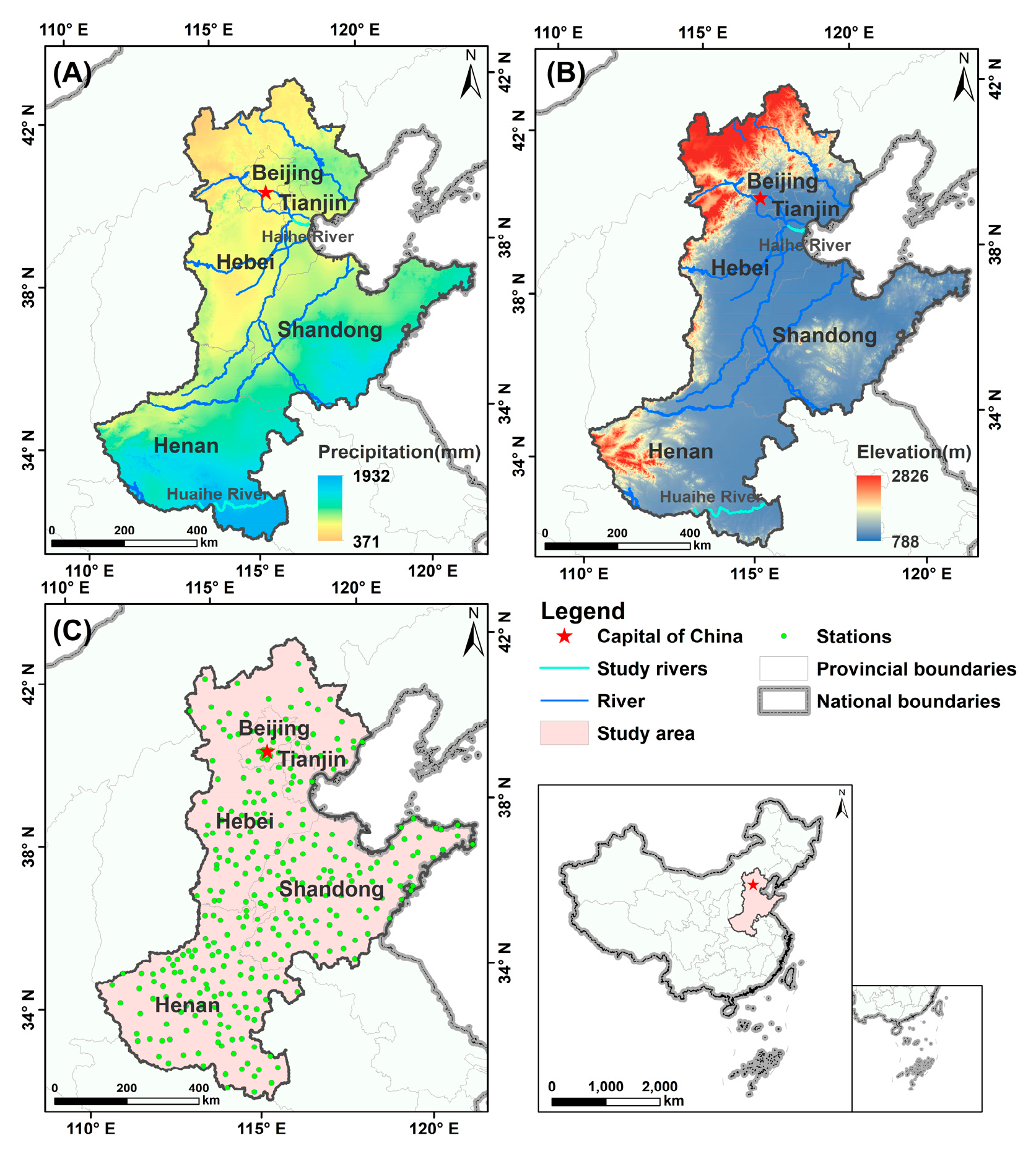
2.1. Overview of the Study Area

Located in central–eastern China, the 3H Plain is bounded in the north by the Yanshan Mountains, in the west by the Taihang Mountains, in the east by the Bohai Sea and the Yellow Sea, and in the south by the Huai River. Including some or all of the Beijing, Tianjin, Hebei, Shandong, and Henan regions, it is an alluvial plain formed by the intermittent flooding of the Yellow River, Huaihe River, and Haihe River (see Figure 1). The 3H Plain is one of China’s essential grain bases, producing summer maize and winter wheat. The region has a typical temperate monsoon climate, with an average annual temperature of 8–15 °C and an average yearly precipitation of 734.9 mm, mainly concentrated from July to September. The annual rainfall is 500–900 mm, decreasing from southeast to northwest due to the influence of the southeast monsoon. Only 20–30% of this precipitation can be used for agricultural production, which is far from meeting the demand for food production. Therefore, a significant amount of supplemental irrigation is still needed annually to ensure food production.

As one of the main winter wheat production areas in China, the Huang-Huai-Hai Plain accounts for approximately 75% of the country’s total winter wheat output [72]. The average yield potential for winter wheat in this region ranged between 5000 and 8000 kg/ha from 1981 to 2008, while the most recent attainable potential yield was 12,611 kg/ha between 2018 and 2019 [73]. In terms of wheat cultivation, Henan Province and Shandong Province have the largest planting areas and highest yields, accounting for 68% of the wheat planting area and 59% of the wheat yield in the Huang-Huai-Hai Plain. Beijing and Tianjin have very small wheat planting areas and yields.

2.2. Data Introduction

2.2.1. Normalized Vegetation Index (NDVI)

The NDVI data used in this study come from two data sources: MODIS L1B remote sensing data and NOAA/AVHRR data, which are described below.

(1)

MODIS Remote Sensing Data

Moderate-Resolution Imaging Spectroradiometer (MODIS) is one of the primary sensors carried on the TERRA and AUQA satellites of the Earth Observing System (EOS) program implemented by NASA. The MODIS sensor has a total of 36 discrete spectral bands ranging from visible to thermal infrared, and MODIS data provide information on land, cloud, ocean, plant, temperature, and climate characteristics, among others, simultaneously for long-term observations of the land surface, biosphere, solid Earth, atmosphere, and oceans. Compared with traditional NOAA/AVHRR, SPOT, and TM data, the data are vastly improved in terms temporal resolution, spectral resolution, update frequency (update time is two days), and broad spectral range (0.4–14.4 um), and are more timely in detecting the ground surface, and thus have been widely used in the monitoring of climate change, natural disasters, the study of land-use change, etc. MODIS data products are divided into calibration data and data products that monitor the land surface, biosphere, solid Earth, atmosphere, and oceans. The data products in the data are mainly divided into four categories—correction, land, sea, and atmospheric data products—and are usually divided by MODIS data processing level (divided into level 0, level 1, level 2, level 3, level 4, and level 5). Levels 0–5 comprise the original data, with a layer-by-layer method of processing and correction used to obtain different products.

(2)

GIMMS NDVI Data Processing

The GIMMS NDVI 3g.v1 dataset (GIMMS NDVI 3g.v1, available https://iridl.ldeo.columbia.edu/SOURCES/.NASA/.ARC/.ECOCAST/.GIMMS/.NDVI3g/.v1p0/, accessed on 15 April 2024) eliminates the effects of volcanic eruption, solar altitude angle, and sensor sensitivity changes over time, making the GIMMS dataset better than other NDVI datasets. GIMMS data are the most extended time series NDVI data available, have a good correlation with other high-resolution datasets, and are widely used around the world.

In terms of data preprocessing to ensure homogeneity and reliability, a variety of specialized techniques were employed. For the AVHRR set, these included actions such as radiometric fine-tuning, cloud detection and subsequent removal, adjustments for atmospheric interference, addressing satellite drift, and applying BRDF (Bidirectional Reflectance Distribution Function) computations. In the context of the MOD09GA dataset, a series of preparatory steps were undertaken, including, but not limited to, quality verification, image stitching, data subsetting, and alterations in data formatting and projection. Such practices were indispensable for procuring a unified and reliable NDVI dataset ripe for further analytical exploration.

To aggregate the daily observations into ten-day and monthly data, we utilized the maximum-value composite (MVC) methodology. This approach was crucial in mitigating the influence of clouds and other forms of noise within the daily images, thereby enhancing the fidelity of the vegetation behavior over the duration of the study.

2.2.2. Meteorological Data

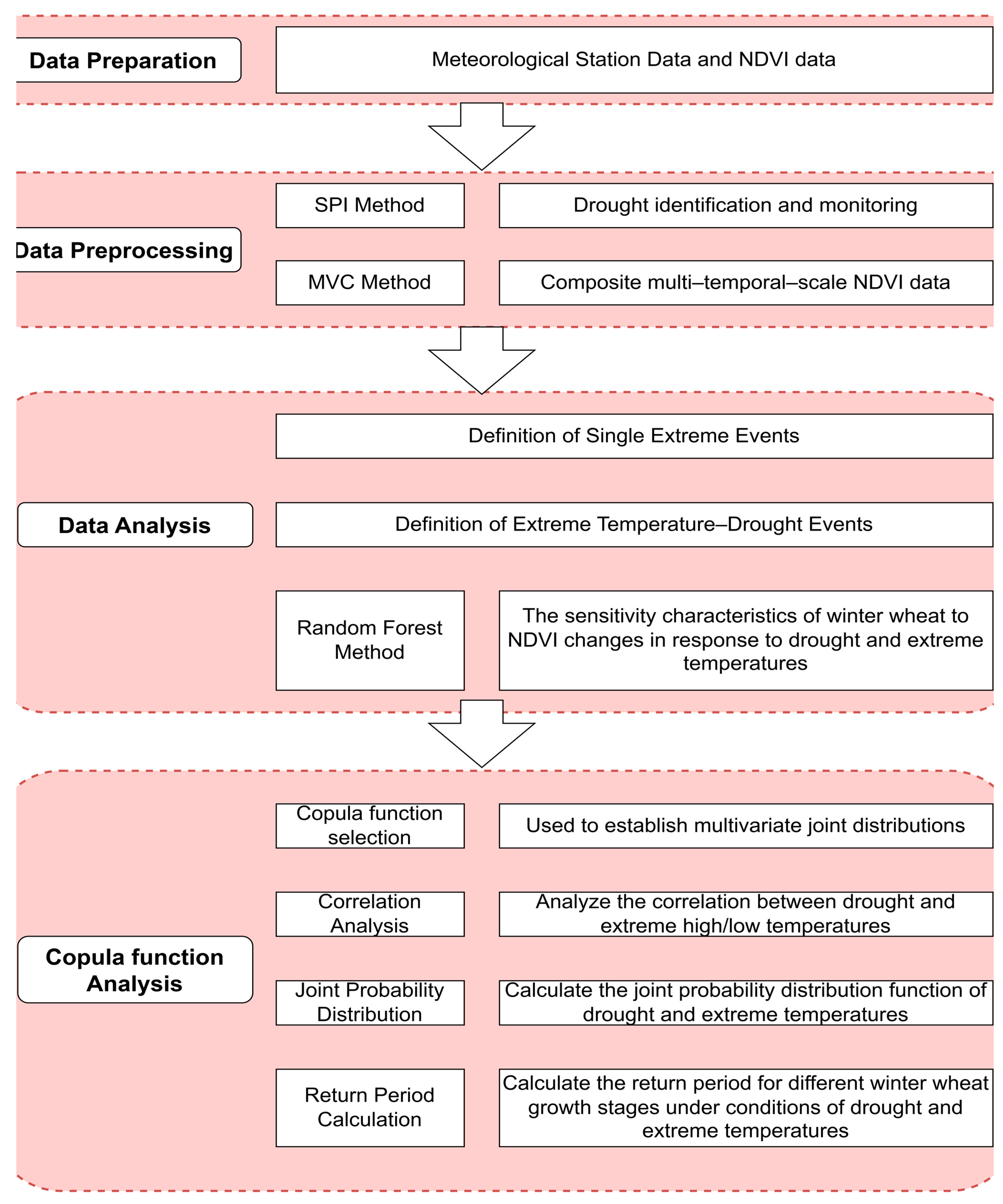
Meteorological data were day-by-day meteorological station data from 1982 to 2021, and were obtained from the China Meteorological Administration (CMA). Firstly, we carried out quality control of the data and selected stations that met the research requirements based on the time length, spatial coverage, and data integrity of the observed data, and a total of 309 station data were selected in the study area. The data elements for each observation station included daily maximum temperature, minimum temperature, average temperature, and precipitation. The Huang-Huai-Hai Plain receives an annual precipitation of 500 to 900 mm, with no more than 30% of the annual precipitation occurring during the winter wheat-growing season. Due to the evapotranspiration during the winter wheat-growing season exceeding the amount of precipitation, the water required for winter wheat mainly relies on groundwater irrigation. Additionally, the Huang-Huai-Hai Plain is one of the most drought-affected regions in China, causing severe negative impacts on winter wheat production [74].

The time ranges of the winter wheat-growing season, the pre-wintering period, and the post-wintering period were classified according to the agricultural zoning of the 3H Plain and the growth pattern of winter wheat, i.e., the growing season of winter wheat is from October to June of the following year, the pre-wintering period is from October to February of the following year, and the post-wintering period is from March to June of the following year.

2.3. Methods

This study employs various methods, including the SPI, the maximum-value composite (MVC) method, copula function, the definition of single extreme events, the definition of extreme temperature–drought events, and random forest, to analyze the spatiotemporal dynamic evolution characteristics of composite drought events during the winter wheat-growing season in the Huang-Huai-Hai Plain, as well as the response of winter wheat to these composite drought events. An introduction to these methods can be found in

Table 1. Methodology overview.

Stage	Method	Reason for Using this Method
Data Processing	SPI Method	The Standardized Precipitation Index (SPI) was chosen as the indicator for drought identification and monitoring, based on the climatic characteristics of the region and data availability. Its flexible time scales allow it to accommodate various research needs, and its simple calculation makes it well suited for the 3H Plain.
	MVC Method	The maximum-value composite (MVC) method was used to generate annual, seasonal, and monthly NDVI values, eliminating the effects of clouds and solar zenith angle, and thereby improving image quality.
	Copula Method	The copula function model was used to create a multidimensional joint distribution. By utilizing marginal distributions and correlation structures, commonly used copula functions were selected for correlation modeling.
	Random Forest Method	The random forest method was used to analyze the sensitivity changes of vegetation (NDVI) to drought and extreme temperatures across multiple time scales, providing high classification accuracy and processing efficiency.
Data Analysis	Definition of Single Extreme Events	Based on research advancements both domestically and internationally, and considering the drought and climatic characteristics of the 3H Plain, single extreme events were defined.
	Definition of Extreme Temperature–Drought Events	Composite events were identified based on the conditions of high temperature and drought or low temperature and drought, and their impacts on winter wheat growth were interpreted.

and Figure 2.

2.3.1. Standardized Precipitation Index (SPI)

The Standardized Precipitation Index (SPI) was selected as the index for identifying and monitoring drought in this study, considering the climatic characteristics of the study area, the scientific validity and authoritative nature of the index, the accessibility of the data required for calculation, and the complexity of the calculation.

Climatic characteristics: The 3H Plain region features a warm–temperate monsoon climate, with annual precipitation ranging from 500 to 1000 mm. Precipitation plays a crucial role in the region’s water resources and agricultural production. The SPI, primarily based on rainfall, can accurately reflect the drought conditions in the 3H Plain region and depict the region’s drought characteristics—something unattainable by other comprehensive drought indices.

Scientific nature of the index: The SPI is flexible in terms of time scales, allowing for the selection of various durations—such as 1, 3, 6, or 12 months—to meet diverse research needs. On the other hand, the PDSI, SC-PDSI, and SPEI time scales are more difficult to deal with. It is difficult to change the calculation time scale conveniently and flexibly, for example, changing the SPI to monitor droughts at different time scales, and the selection of time scales will be limited by data elements and calculation methods. In addition, the PDSI and SC-PDSI methods do not fully consider precipitation in their calculations and focus more on soil moisture and evapotranspiration, which are the essential meteorological factors affecting drought in many areas, limiting their ability to portray drought, while the SPEI accurately does so. However, it takes into account precipitation, but also needs to take into account temperature and potential evapotranspiration, which makes the calculation more complicated.

Authority of the index: The SPI, recommended by the World Meteorological Organization as the international standard for drought monitoring, is widely recognized for its scientific validity and authority. In comparison, the SPI is far more standardized than other indices.

Accessibility of calculation data: The calculation of the SPI is simple and only requires long-term, high-quality precipitation observation data. The 3H Plain is rich in precipitation data and has an extended historical dataset that fully meets the calculation needs of the SPI, which is another advantage of the application of the SPI in this region. The calculation of other drought indices often requires the integration of several meteorological factors, such as temperature, wind speed, relative humidity, evaporation, etc., and requires sufficient and high-quality related observation datasets, which are not easy to obtain in many regions, limiting application in areas with a lack of data.

Computational complexity: The SPI is simple to compute with low data requirements. In contrast, the PDSI and SC-PDSI methods, calibrated for the U.S. Midwest’s Great Plains, require complex regional adaptations, increasing their application difficulty. The SPEI also faces challenges with parameter selection and corrections.

In summary, the SPI is based on precipitation elements, simple calculations, flexible time scales, and robust science, which makes it very suitable to be used for the 3H Plain and other regions where precipitation is more concentrated and vital, as it can better reflect the drought change situation at different time scales in the area. The standardized precipitation index (SPI) is suitable for the study of drought at different time scales, and its foremost step is first to count the precipitation in the studied period, obtain the plant probability distribution, and then carry out typical standardization to obtain the standardized precipitation index. The calculation steps are as follows [75]:

• For some random independent precipitation data x, the mean precipitation and standard deviation for the time period need to be obtained first:

$$\overline{x}=\frac{\sum x}{N} S=\sqrt{\frac{\sum {(x-\overline{x})}^2}{N}}$$

(1)

where N is the number of samples of that precipitation.

2.

Calculate the given precipitation skewness based on the mean precipitation and standard deviation for that time period:

$$Skew=\frac{N}{(N-1)(N-2)}\sum {\left(\frac{x-\overline{x}}{S}\right)}^3$$

(2)

3.

The precipitation data information is then transformed into lognormal values to calculate the gamma distribution statistic U, shape parameter β, and scale parameter α:

$$U=\overline{x_{ln}}-\frac{\sum \mathrm{l}\mathrm{n}\left(x\right)}{N}$$

(3)

$$\beta =\frac{1+\sqrt{1+4U/3}}{4U}$$

(4)

$$\alpha =\frac{\overline{x}}{\beta }$$

(5)

4.

Based on the resulting shape and scale parameters, the cumulative probability of this precipitation data can be calculated and the cumulative probability is

$$G\left(x\right)=\frac{{\int }_0^x{x}^{\alpha -1}{e}^{\frac{-x}{\beta }}dx}{{\beta }^{\alpha }\mathsf{\Gamma }\left(\alpha \right)}$$

(6)

5.

Since the gamma function is not defined when x is 0, and the rainfall in the region at a given time may again be 0 mm, the cumulative probability becomes

$$H\left(x\right)=q+(1-q)G\left(x\right)$$

(7)

where q may be 0; so, the standardized precipitation index is

$$SPI=S\frac{t-\left(c_{2}t+c_1\right)t+c_0}{\left[\left(d_{3}t+d_2\right)+d_1\right]t+1.0}$$

(8)

where $t=\sqrt{ln\frac{1}{{G\left(x\right)}^2}}$; x is the amount of precipitation during the time period, mm; G(x) is the cumulative probability corresponding to x; and S is the positive or negative coefficient of the probability density. S = 1 when G(x) > 0.5; S = −1 when G(x) ≤ 0.5; $c_0$ = 2.515517, $c_1$ = 0.802853, $c_2$ = 0.010328, $d_1$ = 1.432788, $d_2$ = 0.189269, $d_3$ = 0.001308.

In this study, drought classifications were made using the cumulative frequency distribution of labelled precipitation, and the SPI was classified into five drought classes based on the International Meteorological Drought Classification Standard (IMDCS), with reference to

Table 2. SPI drought classification.

Drought Index	Drought Level
	No Drought	Light Drought	Moderate Drought	Severe Drought	Extreme Drought
SPI (dimensionless)	$(-0.5,+\mathrm{\infty }]$	$(-1.0,-0.5]$	$(-1.5,-1.0]$	$(-2.0,-1.5]$	$(-\mathrm{\infty },-2.0]$

.

In this study, the Standardized Precipitation Index (SPI) was used to classify drought levels and assess their impact on winter wheat growth. The SPI classifications range from no drought to extreme drought, each with distinct impacts on winter wheat:

• No drought (SPI > −0.5): Winter wheat growth is unaffected and normal yields can be expected.
• Light drought (−1.0 < SPI ≤ −0.5): Winter wheat experiences minor stress, which may slow growth rates but generally does not lead to significant yield losses.
• Moderate drought (−1.5 < SPI ≤ −1.0): Winter wheat faces moderate stress, with noticeable reductions in growth and potential yield losses.
• Severe drought (−2.0 < SPI ≤ −1.5): Winter wheat undergoes severe stress, resulting in significant reductions in growth and substantial yield losses.
• Extreme drought (SPI ≤ −2.0): Winter wheat experiences extreme stress, with a high risk of crop failure due to severe water deficits.

2.3.2. Maximum-Value Composite Method

To obtain the NDVI composites on annual, seasonal, and monthly scales, researchers used the internationally accepted max-value composite (MVC) method to generate NDVI values for the corresponding periods on annual, seasonal, and monthly scales. A composite (MVC) is used to generate an NDVI value for the corresponding period. This process can eliminate the effects of clouds, atmosphere, and solar altitude, and improve the image quality. In this study, based on the daily data of the NDVI, the maximum-value composite method was used to obtain the monthly maximum NDVI [76], and the calculation formula is as follows:

$${NDVI}_i=Max\left({NDVI}_{ij}\right)$$

(9)

where ${NDVI}_i$ is the NDVI value for month i, and ${NDVI}_{ij}$ is the NDVI value for day j of month i.

2.3.3. Copula Function

Sklar introduced copula functions [77], which can model multidimensional joint distributions through marginal distribution and correlation frameworks [78]. Multiple copula functions can be used to build multidimensional joint distributions of climate factors and drought. In this study, five types of copula function clusters were selected [79,80,81,82,83]: (1) Clayton, (2) Frank, (3) Gaussian, (4) Gumbel, and (5) t. Due to the excellent performance of these five copula function clusters, they were the first choice for correlation modeling.

Parameter Estimation

Non-parametric methods were used in the study to estimate the parameters of the copula functions, as specified in the form of various copula function references.

The relationship between $\theta$ and $\tau$ (Kendall correlation coefficient) is demonstrated in the above

Table 3. Copula function clusters and their mathematical descriptions.

Copula Function Name	Mathematical Description
Clayton	$\max {(u^{-\theta }+v^{-\theta }-1.0)}^{-1/\theta }$
Frank	$-\frac{1}{\theta }\ln [1+\frac{(\exp \left(-\theta u\right)-1)(\exp \left(-v\theta \right)-1)}{\exp \left(-\theta \right)-1}]$
Gaussian	${\int }_{-\infty }^{{\varphi }^{-1}\left(u\right)}{\int }_{-\infty }^{{\varphi }^{-1}\left(v\right)}\frac{1}{2\pi \sqrt{1-{\theta }^2}}\exp \left(\frac{2\theta xy-x^2-y^2}{2(1-{\theta }^2)}\right)dxd{y}^b$
Gumbel	$\exp (-{[{(-\ln (u\left)\right)}^{\theta }+{(-\ln (v\left)\right)}^{\theta }]}^{\frac{1}{\theta }})$
t	${\int }_{-\infty }^{t_{{\theta }_2}^{-1}(u)}{\int }_{-\infty }^{t_{{\theta }_2}^{-1}(v)}\frac{r\left(\right({\theta }_2+2)/2)}{r({\theta }_2/2)\pi {\theta }_2\sqrt{1-{\theta }_1^2}}\exp \left(\frac{2\theta xy-x^2-y^2}{2\left(1-{\theta }^2\right)}\right)dxd{y}^b$

. Accordingly, $\tau$ is calculated and the corresponding joint distribution parameters are obtained. The formula is given below:

$$\tau =1-\frac{1}{\theta }$$

(10)

Validation and Evaluation

In order to quantitatively assess the fitting error and select the appropriate copula function, the Akaike information criterion (AIC) and the Bayesian information criterion (BIC) [83] were used as the criteria for selecting the copula function clusters.

$$AIC=-2l\left(\widehat{\theta }|y\right)+2k$$

(11)

$$BIC=-2l\left(\widehat{\theta }|y\right)+Kln\left(n\right)$$

(12)

Correlation Analysis and Marginal Distribution Function

This study aims to determine whether there is a correlation between drought and extremely high and low temperatures, establish a joint distribution function, and analyze the correlation between drought and climate factors using Kendall, Pearson, and Spearman rank correlation coefficients, respectively. The paper uses MCMC (Markov chain Monte Carlo) simulations to estimate the parameters of the copula function, study the dependence structure relationship between the variables, and to screen the optimal marginal distribution function for each variable.

Joint Probability Distribution

To investigate the joint probability of drought and extreme high and extreme low temperatures, respectively, the marginal distribution functions of the three are first calculated, and the parameters of the corresponding functions are determined. The fitting results of the functions are evaluated using a QQ plot (Quantile–Quantile plot). The two-dimensional copula function is constructed based on the univariate edge function, and the optimal type of copula function is selected among the copula function clusters based on the three goodness-of-fit evaluation metrics, namely, AIC, BIC, and RMSE.

Return Period Calculation

The reproduction period is when a random variable appears in a more extended period [84]. Calculating the return period under drought and extreme temperature conditions for different winter wheat fertility periods provides more detailed information for an in-depth investigation of how extreme temperature and drought affect winter wheat. Univariate return intervals or return periods may lead to the overestimation or underestimation of the risk rate of an event.

Therefore, this study calculates the bivariate joint and conditional return periods [85,86]. The joint return period is defined as $X\ge x \mathrm{a}\mathrm{n}\mathrm{d} Y\ge y$, and the conditional return period is defined as $X\ge x \mathrm{o}\mathrm{r} Y\ge y$.

$$T_{joint}=\frac{E\left(L\right)}{P(X\ge x,Y\ge y)}=\frac{E\left(L\right)}{1-F_X\left(x\right)-F_Y\left(y\right)+C(F_X\left(x\right),F_Y(y\left)\right)}$$

(13)

$$T_{conditional}=\frac{E\left(L\right)}{P(X\ge x or Y\ge y)}=\frac{E\left(L\right)}{1-C(F_X\left(x\right),F_Y(y\left)\right)}$$

(14)

where T_joint denotes the joint return period; T_conditional denotes the conditional return period; and E(L) is the expected value of the time interval between the start of the consecutive events. The relationship between the univariate, bivariate and correlated return periods can be found in the corresponding source [87].

2.3.4. Random Forest

In recent decades, in the context of global warming, the Huang-Huai-Hai Basin has experienced a significant increase in temperature. Consequently, the sensitivity of vegetation growth to drought and extreme temperatures may exhibit variation. To examine the changes in the sensitivity of vegetation (NDVI) to drought and extreme temperatures, the study employs the random forest method to analyze the multi-temporal-scale variation in vegetation (NDVI) in response to drought and extreme temperatures. The algorithm of the random forest is as follows [88]:

(1)

Using the bootstrap method with replacement, randomly select n groups of sample data from the initial training set to construct decision trees.

(2)

Among the multiple attribute features of the training samples, select the optimal feature for splitting each time. Each tree continues this splitting process until all training samples under that node belong to the same category.

(3)

To fully utilize the classification ability of each tree, allow each tree to grow to its maximum extent without any pruning.

(4)

Combine the generated multiple classification trees to form a random forest, and use voting to determine the final classification result.

To quantify the effectiveness of the classification, use the ensemble of the classification trees ($h_1\left(x\right)$,$h_2\left(x\right)$, ...,${ h}_k\left(x\right)$) and the training set obtained according to the distribution of random vectors X and Y. Define the margin maximization function as

$$mg\left(X,Y\right)=\alpha {\nu }_{k}I\left(h_k\left(X\right)=Y\right)-\genfrac{}{}{0pt}{}{max}{j\ne Y}\alpha {\nu }_{k}I\left(h_k\left(X\right)=j\right)$$

(15)

In the equation, I(g) is the indicator function and $\alpha {\nu }_k$ is the average number of votes for the obtained category. The margin maximization function calculates the extent to which $\alpha {\nu }_k$ in I(g) surpasses the voting results of all other categories. The larger the value of the margin function, the better the classification effect. Due to the strong rule of the law of large numbers followed by classification trees, the normalized error decreases with the increase in the number of classification trees. However, when the number of classification trees is too large, the effect of reducing the normalized error becomes less significant, while the computational load and processing time increase. The random forest algorithm demonstrates high classification accuracy and processing efficiency for large datasets and exhibits strong adaptability to various types of sample data. It is highly capable of handling both discrete and continuous data, and the data do not need to be normalized. During the growth process of random forest classification trees, the algorithm continuously selects the optimal attributes for splitting and performs pruning on the classification trees to further reduce computation.

2.3.5. Definition of Extreme Temperature–Drought Compound Events

Considering the drought and climatic characteristics of the Huang-Huai-Hai Plain, this study identifies extreme-high-temperature–drought and extreme-low-temperature–drought compound events on a monthly scale using meteorological station observations. Therefore, the definitions of extreme temperature–drought compound events in this study are as follows:

(1) 

Definition of High Temperature–Drought Compound Events:

• High-Temperature Event Standard: A high-temperature event is defined as when the maximum temperature is not lower than the 90th percentile threshold of historical maximum temperatures. This means that when the maximum temperature for a given month exceeds or equals the highest 10% of historical maximum temperatures for that month, a high-temperature event is considered to have occurred.
• Drought Event Standard: The drought event standard uses the Standardized Precipitation Index (SPI). A drought event is considered to have occurred when the SPI value indicates mild drought or worse. Mild drought conditions typically correspond to SPI values less than −0.5.
• High-Temperature–Drought Compound Event: When both the high-temperature event and drought event standards are met simultaneously, i.e., the maximum temperature reaches or exceeds the 90th percentile threshold and the SPI value is less than −0.5, a high-temperature–drought compound event is considered to have occurred.

(2) 

Definition of Low-Temperature–Drought Compound Events:

• Low-Temperature Event Standard: A low-temperature event is defined as when the minimum temperature is not higher than the 10th percentile threshold of historical minimum temperatures. This means that when the minimum temperature for a given month is below or equals the lowest 10% of historical minimum temperatures for that month, a low-temperature event is considered to have occurred.
• Drought Event Standard: Similar to the high-temperature–drought compound event, the drought event standard uses the Standardized Precipitation Index (SPI). A drought event is considered to have occurred when the SPI value indicates mild drought or worse. Mild drought conditions typically correspond to SPI values less than −0.5.
• Low-Temperature–Drought Compound Event: When both the low-temperature event and drought event standards are met simultaneously, i.e., the minimum temperature reaches or falls below the 10th percentile threshold and the SPI value is less than −0.5, a low-temperature–drought compound event is considered to have occurred.

3. Results

3.1. Response of Winter Wheat to Combined High-Temperature–Drought Events

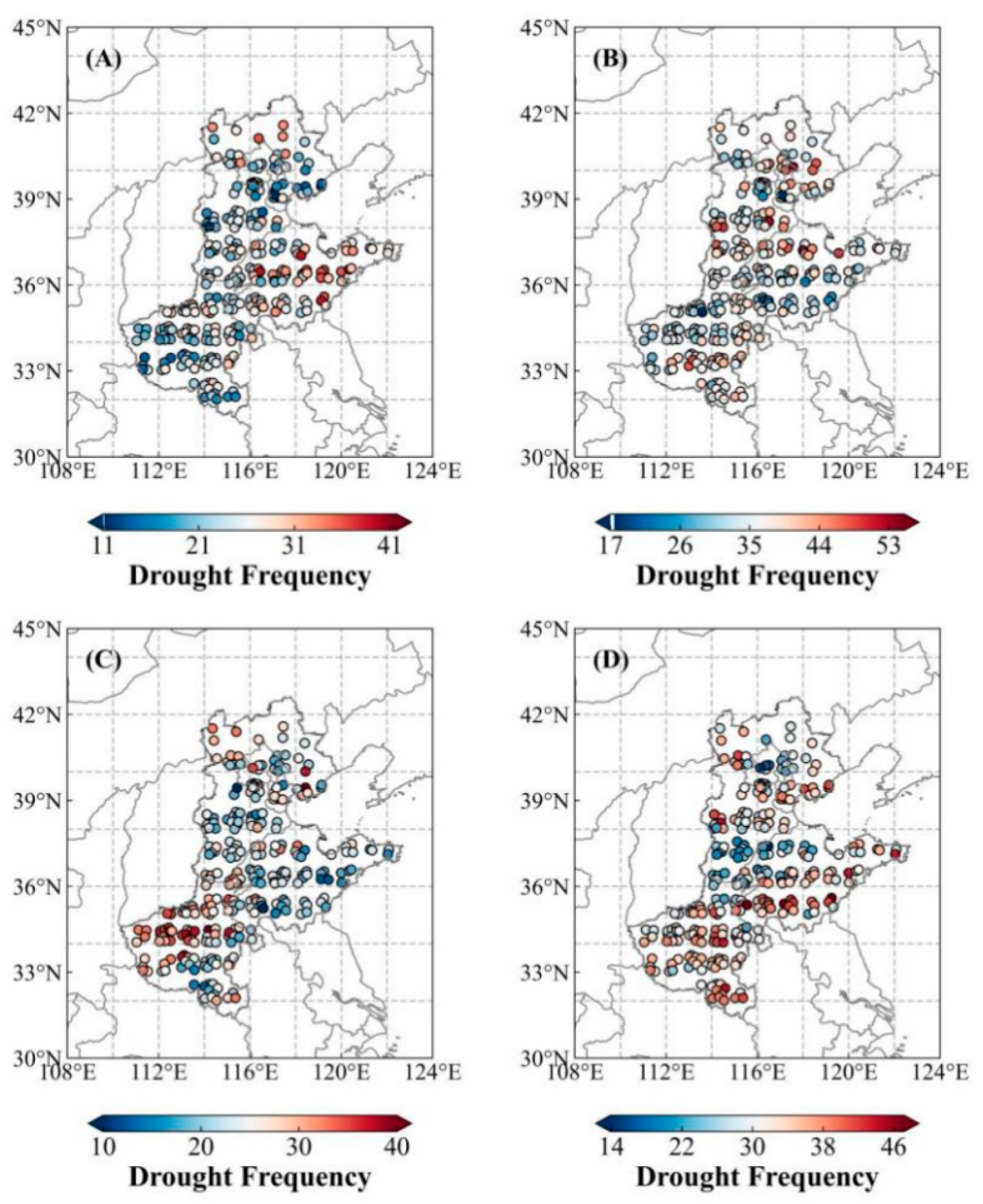
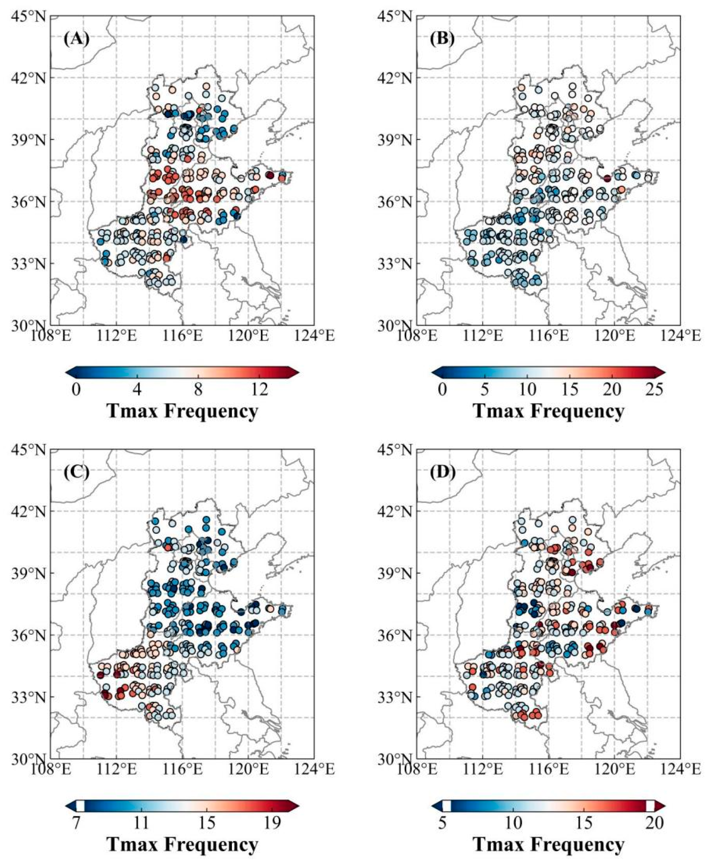
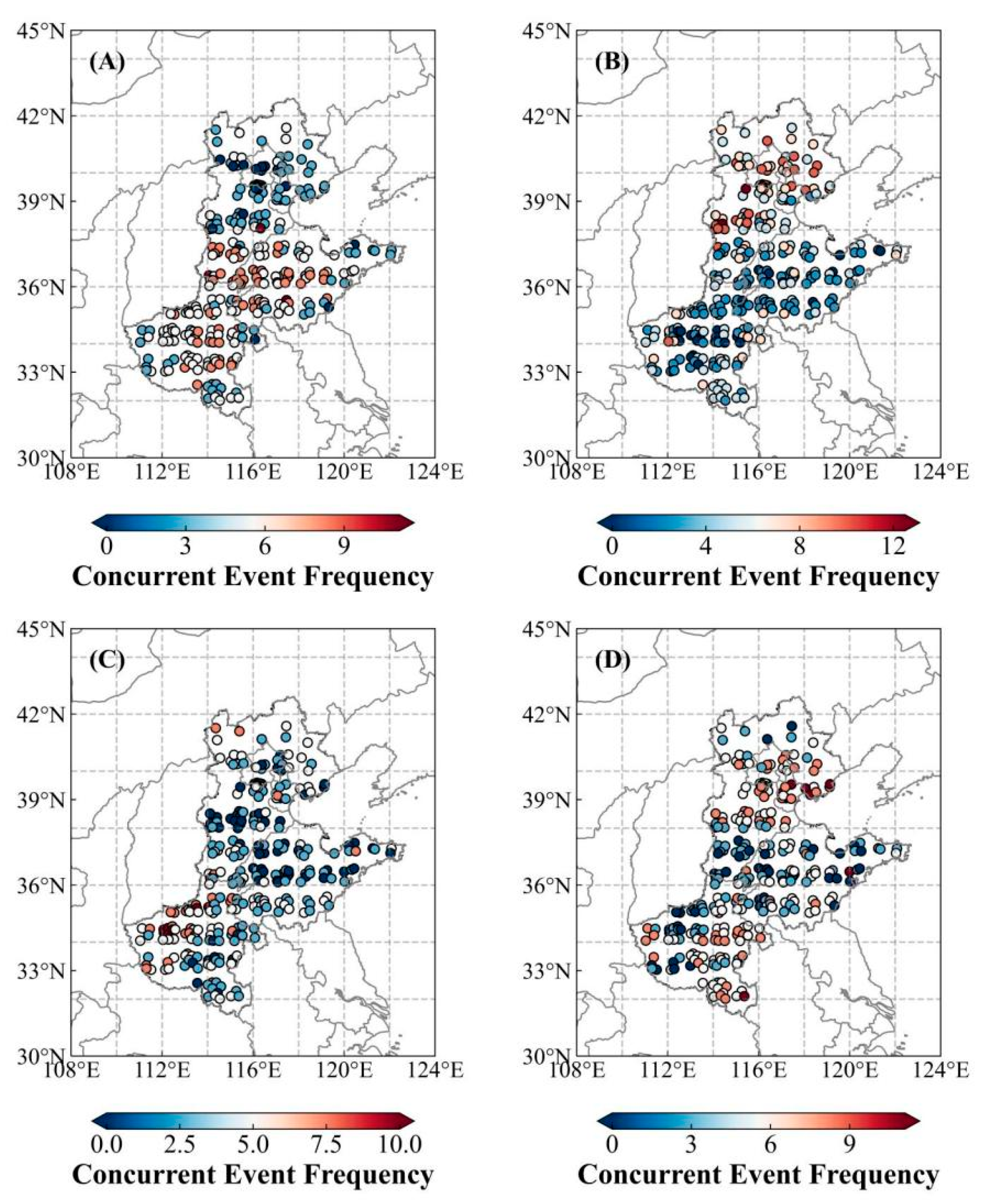
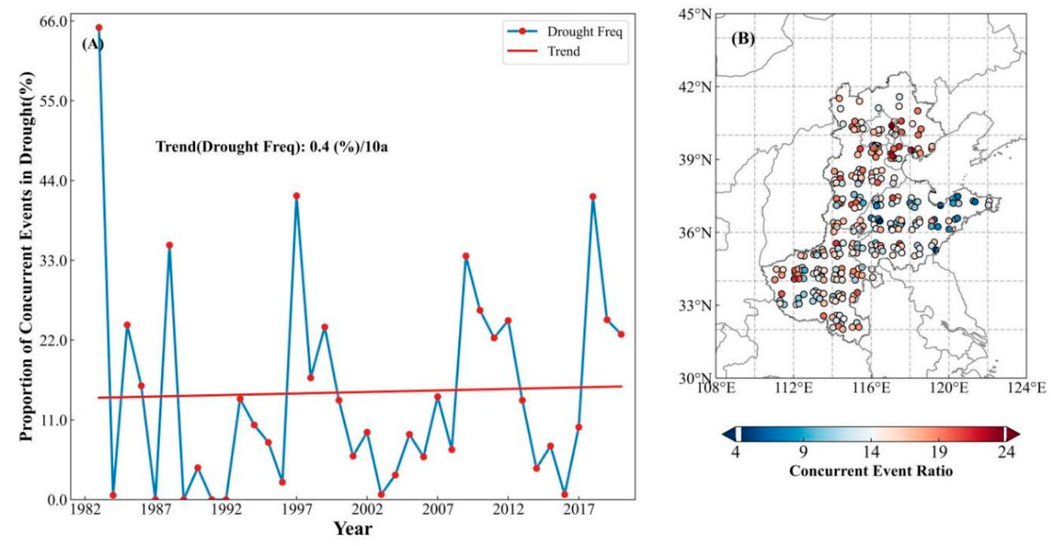
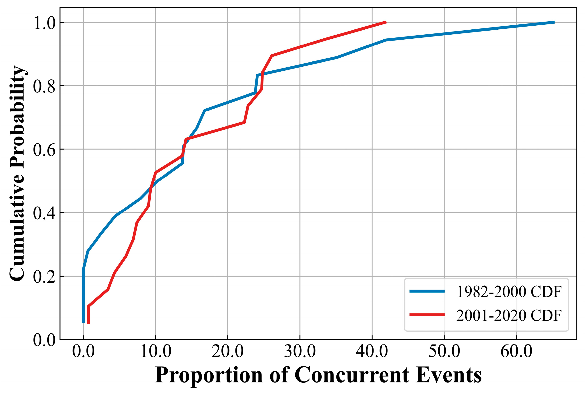
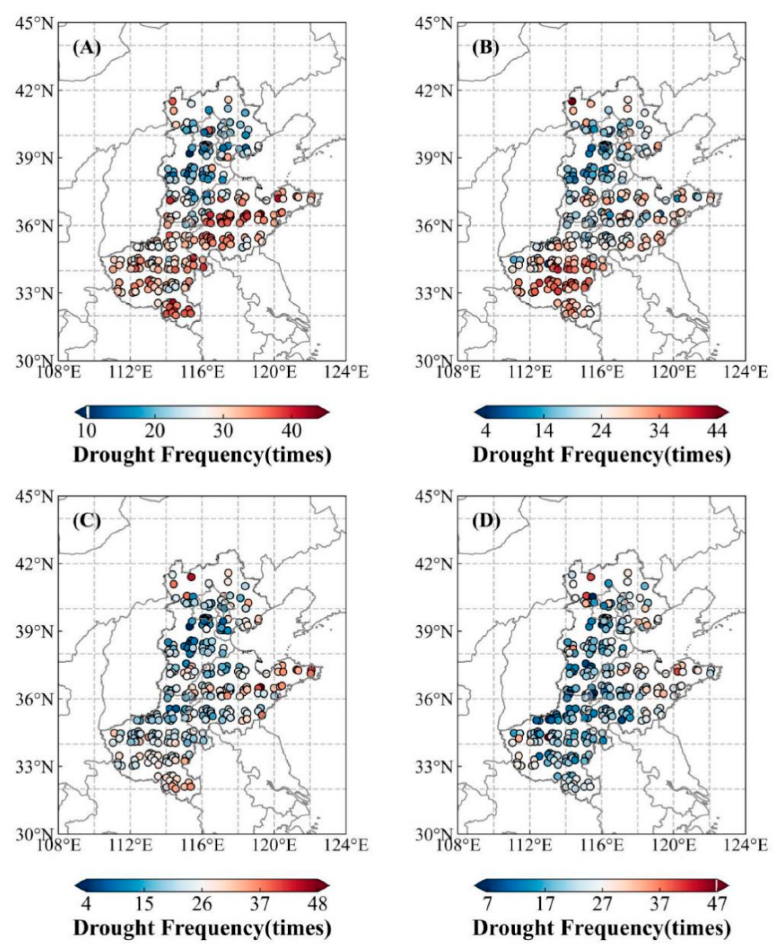
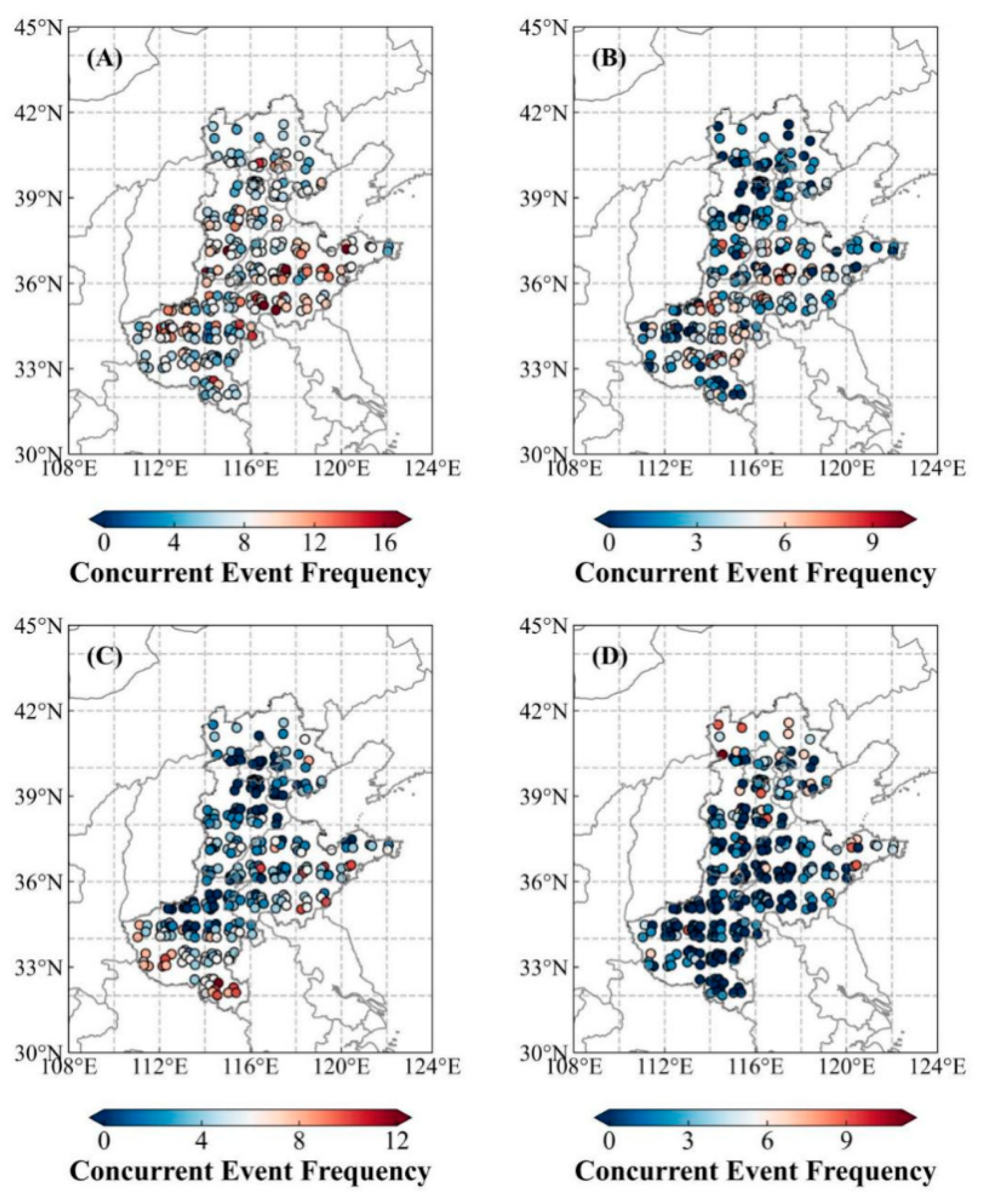
3.1.1. Spatiotemporal Distribution Characteristics of High-Temperature–Drought Compound Events

Figure 3 shows the spatial distribution of drought frequency per decade in the 3H Plain from 1982 to 2020. From 1982 to 1991, the drought frequency in eastern and central Shandong was as high as 40%; some stations in northern Hebei and Henan reached 30%; and Tianjin, Beijing, and central Hebei had the lowest frequencies, at only 10%. The rest of the region had a drought frequency of about 20%. From 1992 to 2001, the probability of droughts reached its highest at 50% in northern Shandong, southern Hebei, Tianjin, and Beijing; the probability was 45% in southern Henan. The lowest frequency, only 20%, occurred in southeastern Shandong and northern Henan; the rest of the regions averaged around 35%. From 2002 to 2011, the frequency of droughts was the highest at 40% in north Henan and eastern Hebei; the second highest frequency, 30%, was observed in northern Hebei, northern Shandong, Beijing, and parts of central and southern Henan. The lowest frequency, at only 10%, was found in southeastern Shandong and central Hebei. From 2012 to 2020, the frequency of drought in southeast Shandong reached its highest at 46%, while for most of Henan, central and southern Shandong, Tianjin, and northern Hebei, frequencies were generally above 35%; the lowest frequencies, at only 15%, were observed in Beijing and southern Hebei. The comprehensive drought frequency maps across these four periods demonstrate that the proportion of regions experiencing droughts in the Huang-Huai-Hai Plain has gradually expanded over the past 39 years, exhibiting a pattern of expansion from north to south. Drought frequencies have significantly increased, especially in Henan and Shandong.

From 1982 to 1991 (Figure 4A), in the 3H Plain, the high-temperature frequency in southern Hebei and western and eastern Shandong reached as high as 10%; in northern Hebei and some stations in central Henan, the second highest frequency was observed at 8%. Beijing experienced the lowest frequency at only 1%, and the rest of the region had a frequency of about 5%. From 1992 to 2001 (Figure 4B), eastern Shandong and eastern and southern Hebei recorded the highest frequency at 15%, followed by northern Hebei and western Shandong at 12%, with Henan having the lowest at 5%. From 2002 to 2011 (Figure 4C), west Henan saw the highest frequency at 20%, followed by selected sites in northern Hebei and northern and southern Henan at 17%; Shandong and most of Hebei had lower frequencies at only 10%. Between 2012 and 2020 (Figure 4D), eastern Shandong, Tianjin, Beijing, western Hebei, and northern and southern Henan recorded the highest frequencies, reaching 20%, followed by north and central Hebei and northern Shandong at 15%; southern Hebei had the lowest, at only 5%. Accordingly, over the past 39 years, the frequency of high temperatures in the Huang-Huai-Hai Plain has shown an overall increasing trend and expanded from north to south. The center of the drought-affected region has shifted from Hebei to Shandong and Henan.

From Figure 5, it can be seen that from 1982 to 1991, the frequency of high-temperature–drought events in central Henan, central and western Shandong, and southern Hebei was as high as 9%; Beijing, Tianjin, and central Hebei had the lowest frequency at 1%, and the rest of the regions experienced a high-temperature–drought frequency of about 5%. From 1992 to 2001, the frequency of high-temperature–drought in central Hebei was the highest at 10%, followed by northern Hebei at 8%, while most of Henan and Shandong had lower frequencies, at around 2%. From 2002 to 2011, north Henan recorded the highest frequency at 10%, whereas southern Hebei, Beijing, northern Shandong, and central Henan had the lowest frequencies, at only 1%. From 2012 to 2020, Tianjin and southern Henan experienced the highest frequency at 10%, followed by central Hebei and central and south parts of Beijing and Henan at 7%; the lowest frequency of 1% was observed in southern Hebei, western and eastern Shandong, and west Henan. Overall, the trend of high temperature–drought has been one of migration from north to south, with disaster areas expanding outward.

Figure 6 shows that in the 3H Plain, the proportion of high-temperature–drought compound events relative to total drought events has gradually increased over the last 40 years (1982–2020), with a growth rate of 0.4% per decade. The proportion of high-temperature–drought compound events also shows significant interannual fluctuations. The proportion peaked at 66% in 1982, followed by 44% in 1997 and 2018. No compound events occurred in 1983, 1987, 1989, 1991, 1992, 2003, or 2016. Additionally, the proportion decreased between 1997 and 2003, and 2009 and 2016, and increased from 2003 to 2009 and 2017 to 2019. Spatially, the Beijing and Tianjin regions recorded up to 20% of the compound events, followed by areas in Hebei and Henan, with up to 18% at most sites. Western and eastern Shandong had the lowest proportion, at only 5%; overall, the region demonstrated a decreasing trend from north to south.

Figure 7 shows that from 1982 to 2020, the Huang-Huai-Hai Plain experienced a 3-month lag between drought and winter wheat according to the Normalized Difference Vegetation Index (NDVI). Most areas of the study region exhibited a negative correlation, with the highest correlation coefficient, −0.5, occurring in northern and southern Hebei and western and northern Shandong. Additionally, most areas in Henan show a negative correlation with a coefficient of −0.3. At a 2-month lag, south and north Hebei and a small part of central Shandong exhibit a positive correlation, with a coefficient of 0.2, while the remaining regions show negative correlations. Regarding the relationship between high temperature and the NDVI, a 3-month lag shows that most of Henan, western Shandong, and southern Hebei have the highest positive correlation, with a coefficient of 0.5.

Conversely, western Henan, eastern Shandong, Tianjin, Beijing, and eastern Hebei demonstrate a negative correlation, with a coefficient of −0.2. With a 2-month lag, southern Henan, western Shandong, and southern Hebei exhibit the highest positive correlation, with a coefficient of 0.5. Conversely, northern Hebei, eastern Shandong, Tianjin, Beijing, and western Henan show a negative correlation, with a coefficient of −0.2. With a 1-month lag, central and southern Henan, west Shandong, and southern Hebei exhibit the highest positive correlation with a coefficient of 0.5. In contrast, northern and central Hebei, Tianjin, Beijing, eastern Shandong, and western Henan show a negative correlation, with a coefficient of −0.2. When considering a 1-month lag for high temperature and the NDVI, the correlation coefficient is −0.2. The regions with the highest positive correlation between high temperature and NDVI are southern and central Henan, Beijing, and northern Hebei, with a coefficient of 0.4. In contrast, east and central Shandong have the highest negative correlation, with a coefficient of −0.3. Overall, for the high-temperature–drought compound events over the past 39 years, the NDVI has shown a negative correlation with drought and a positive correlation with maximum temperature across most of the Huang-Huai-Hai Plain.

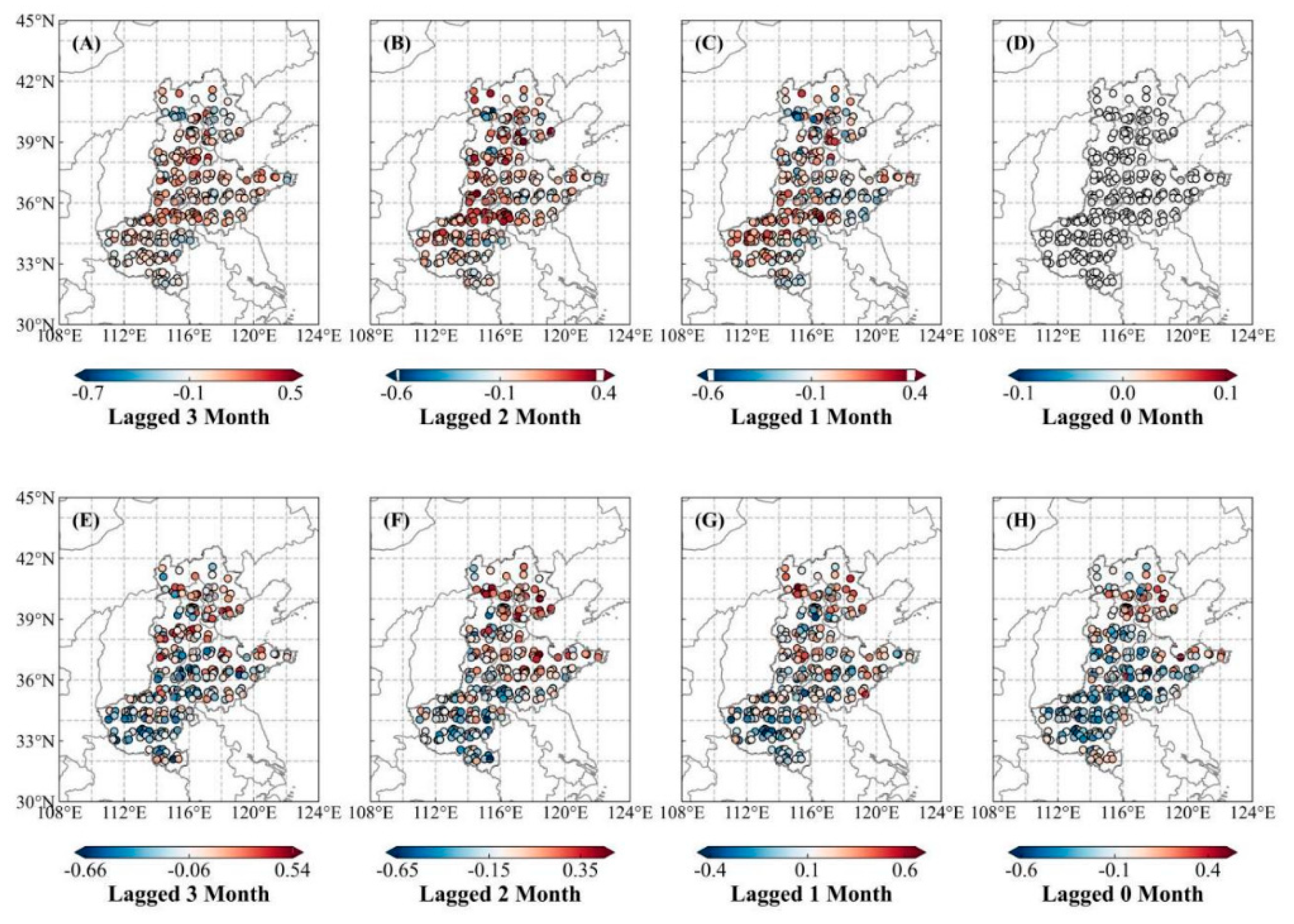
3.1.2. Sensitivity of Winter Wheat to High-Temperature–Drought Compound Events

Figure 8 shows that 40% of the sites experienced high-temperature–drought compound events during the period from 2001 to 2020. For the past 20 years, the shape of the ECDF is a steeply sloped curve, indicating that the data may follow a skewed distribution, and the sites within this interval are more densely clustered, suggesting that the occurrence of compound drought events is relatively concentrated. In contrast, during the period from 1982 to 2000, approximately 60% of the sites experienced high-temperature–drought compound events. When the proportion of sites experiencing compound events is less than 25%, the ECDF curve is relatively steep, indicating that 20% of the sites are relatively concentrated; when the proportion of sites is between 30% and 60%, the curve is relatively flat, indicating that the occurrence of compound drought events is more dispersed.

Figure 9 shows the sensitivity characteristics of winter wheat to variations in high-temperature–drought compound events using the random forest method, we conducted an attribution analysis and obtained Figure 8. According to the sensitivity identification of climate factors for winter wheat in the Huang-Huai-Hai Plain from 1982 to 2020, it is evident that, in high-temperature–drought compound events, winter wheat exhibits the highest sensitivity to maximum temperature, reaching 19%; followed by minimum temperature at 17%; then precipitation at 16%; and the lowest sensitivity to the drought index (SPI), at only 14%. Overall, winter wheat shows a higher sensitivity to temperature-related climate factors compared to precipitation, particularly to maximum temperature.

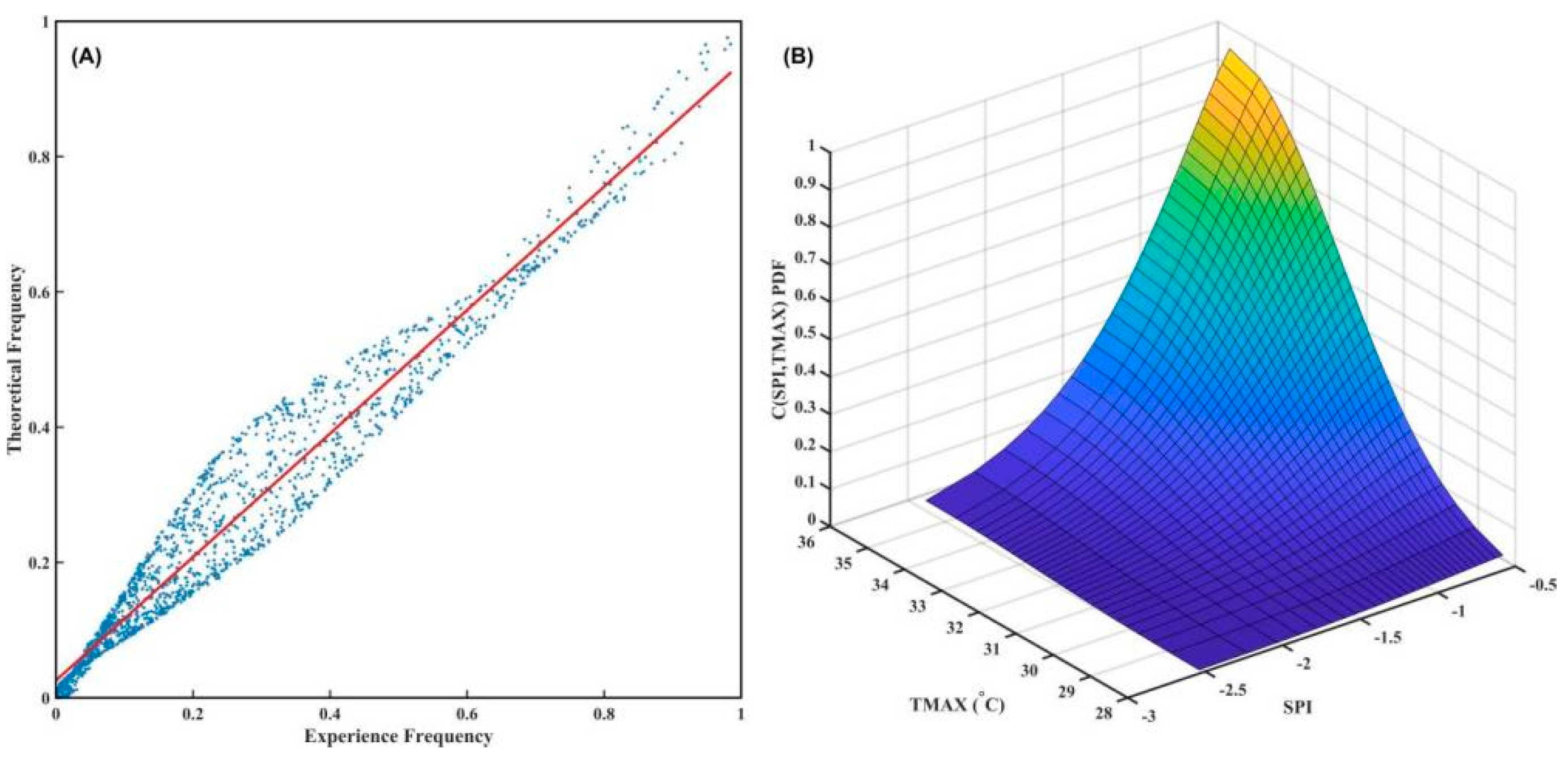
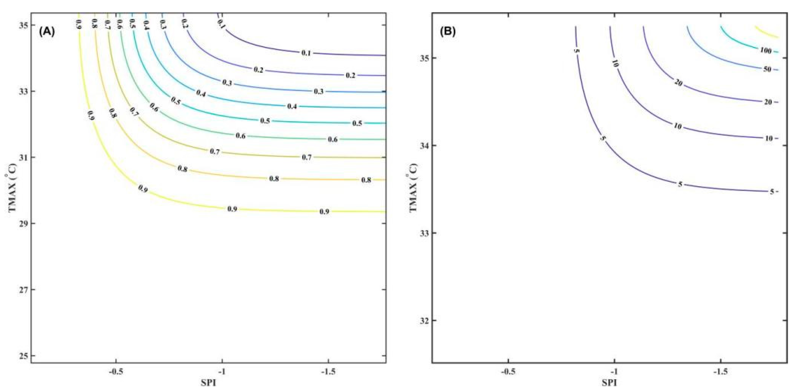
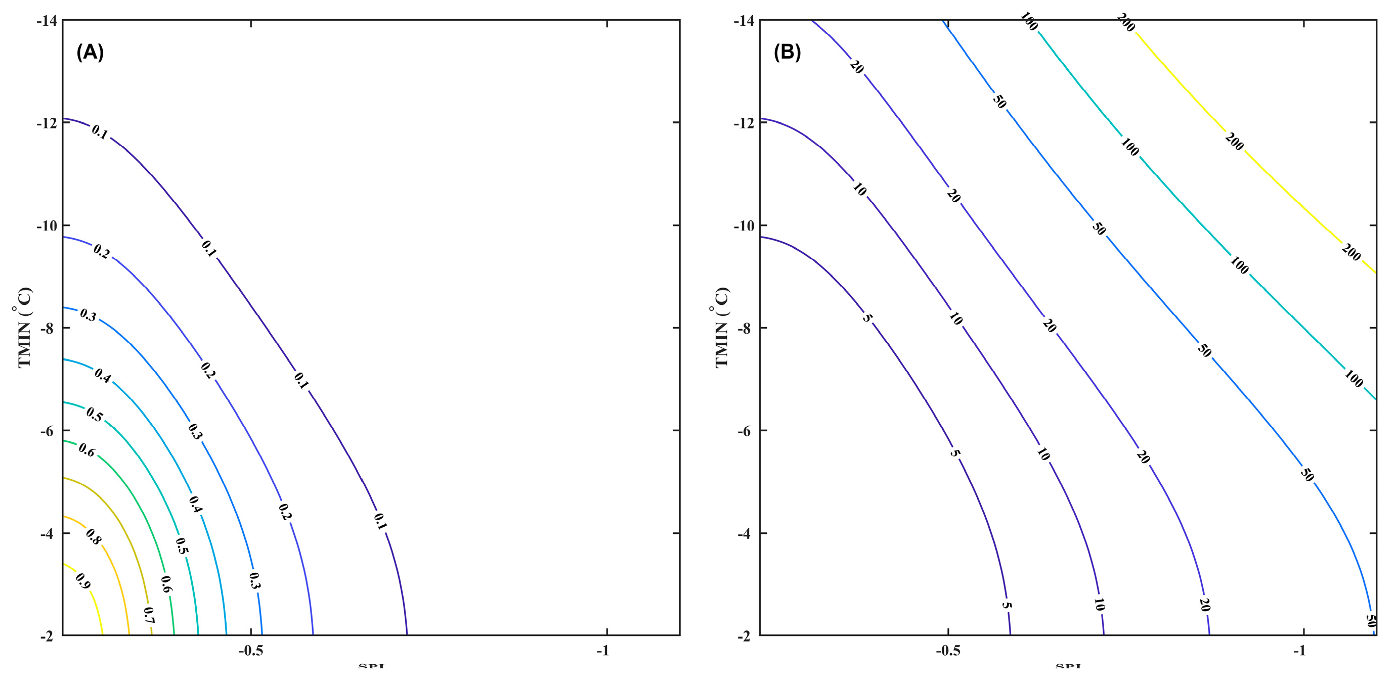
3.1.3. Copula Analysis of High-Temperature–Drought Compound Events

Due to the correlation between high-temperature events and drought events, relying solely on univariate return periods for results may lead to deviations from the actual situation. Therefore, it is necessary to describe the bivariate distribution of these two types of climate hazard events. In this section, the correlation between droughts and extreme high temperatures is examined, and their correlation is measured using the Pearson rank correlation coefficient, Kendall rank correlation coefficient, and Spearman rank correlation coefficient. The results of these calculations are presented in

Table 4. Kendall/Spearman/Pearson rank correlation coefficients for drought (SPI) and extreme heat (TMAX) in the 3H Plain, 1982–2020.

Factors Name	Kendall		Spearman		Pearson
	r	p Value	r	p Value	r	p Value
3H Plain_SPI_TMAX	0.301	0.053	0.400	0.056	0.383	0.082

.

Table 4 shows a positive correlation between drought (SPI) and extreme high temperature (TMAX) in the 3H Plain region, passing the 10% significance level. Given the analysis results, modeling the bivariate distribution of TMAX and SPI with a copula function is feasible.

Table 5. Criteria for cluster selection of copula function for drought–extreme heat in the 3H Plain.

Cop_Family	AIC	BIC	RMSE
Gaussian	14.67	20.19	0.202
t	16.67	27.71	0.199
Clayton	14.63	20.15	0.180
Frank	14.67	20.19	0.198
Gumbel	14.70	20.22	0.223

indicates that in the 3H Plain region, the Clayton copula function is optimal for modeling the TMAX-SPI relationship based on the AIC, BIC, and RMSE evaluation criteria. The values for these evaluation indices are lower for the Clayton copula than for the other four copula functions, suggesting that the Clayton copula offers the best fit and is most suitable for describing the joint distribution of extremely high temperature and SPI. Consequently, the Clayton copula function was selected to establish a two-dimensional joint probability distribution model for extremely high temperatures and drought in the 3H Plain.

Figure 10 depicts the probability distribution function for high-temperature–drought compound events in the 3H Plain from 1982 to 2020. Figure 10A shows that the scatter points, representing actual and theoretical frequencies, closely align with the fitted line. This alignment indicates that the overall trends of the scatter points and the fitted line are completely consistent, effectively capturing the joint distribution characteristics of the SPI and TMAX. Consequently, this demonstrates that the copula model employed accurately reflects the joint behavior of these two variables. Additionally, the model accurately captures the marginal distributions of both the SPI and TMAX. Figure 10B shows that the probability of heat–drought compound events increases with higher maximum temperatures. Similarly, the likelihood of these events also increases as the SPI rises (indicating a decrease in drought intensity). The probability of the compound event changes minimally when temperatures range from 28 to 30 °C and when the SPI is between −2 and −2.5.

Figure 11A illustrates the joint probability distribution between drought and extreme high temperatures in the 3H Plain. This figure allows us to determine the joint probability of extremely high temperatures and drought at any given point, clearly reflecting their correlation across various values. Notable features include the asymmetric and skewed dependence structure in the monthly data, where extremely high temperatures have minimal impact on drought at lower values and significant effects at higher values. The contour plots enable the derivation of the interval distribution for extreme temperatures and drought with joint probabilities ranging from 0.1 to 0.9. The contour plots also reveal an increase in joint probability when either the extremely high temperature is fixed and the drought severity is lower, or the drought severity is fixed and the maximum temperature is lower. Joint probabilities for maximum temperature and SPI vary significantly across different intervals on the same contour. The figure indicates low joint probabilities for very high temperatures with very low or very high SPI scenarios and high joint probabilities for very high temperatures paired with very high SPI values. Heat–drought compound events are more likely to occur under high temperatures and mild droughts.

Figure 11B presents the two-dimensional contour plots of the joint return periods for extremely high temperatures and the SPI in the 3H Plain. Researchers can use the joint return period plot to calculate the return period corresponding to extremely high temperatures or SPI equal to or greater than a specific value. The plots depict combinations of extremely high temperature and SPI equal to or greater than a particular value for return periods of 2, 5, 10, 25, 50, and 100 years. A smaller combined return period corresponds to a more extensive range of values for extremely high temperature and SPI, indicating that when the extremely high temperature is specific, the SPI is more likely to have a shorter return period. High-temperature–drought compound events are more prone to occur during overlapping high temperatures and mild drought periods.

Figure 12A displays a contour plot of the joint probability of exceeding extremely high temperatures and the SPI in the 3H Plain. The figure indicates that with a constant drought level, the joint probability of exceeding the high-temperature–drought compound event decreases as the maximum temperature increases. Conversely, with a continuous maximum temperature, the joint probability of exceeding the compound event decreases as the SPI decreases (indicative of increasing drought intensity). This joint exceedance probability graph enables the determination of the likelihood of any given value of maximum temperature and SPI. The figure shows various combinations of maximum temperature and SPI simultaneously greater than or equal to certain thresholds, with joint exceedance probabilities ranging from 0.1 to 0.9. The graph illustrates that smaller values of maximum high temperature and SPI correlate with higher joint exceedance probabilities and vice versa. This observation suggests that the likelihood of both extreme temperature and the SPI surpassing lower thresholds together is greater than their likelihood of surpassing higher thresholds.

Figure 12B illustrates the co-occurrence return periods for extreme high temperatures and drought in the 3H Plain. When the drought level is fixed, the joint exceedance recurrence period of the compound event increases with the maximum temperature. Similarly, when the extremely high temperature is fixed, the joint exceedance recurrence period increases as the SPI decreases (indicating a strengthening of drought intensity). The recurrence period is also longer when the temperature increases and the drought intensity is weaker. The same exceeding recurrence period plot reveals the recurrence period for which extremely high temperature and SPI are both greater than or equal to a specific value. The figure depicts these combinations for recurrence periods of 2, 5, 10, 25, 50, and 100 years. For cases with extremely high temperature and SPI-fixed values, their co-occurrence return periods are significantly longer than the joint return period. For a given return period, more considerable return periods correspond to higher values of extreme temperature and SPI, and can exceed 100 years when extreme temperature and drought levels are sufficiently high.

3.2. Response of Winter Wheat to Combined Low-Temperature–Drought Events

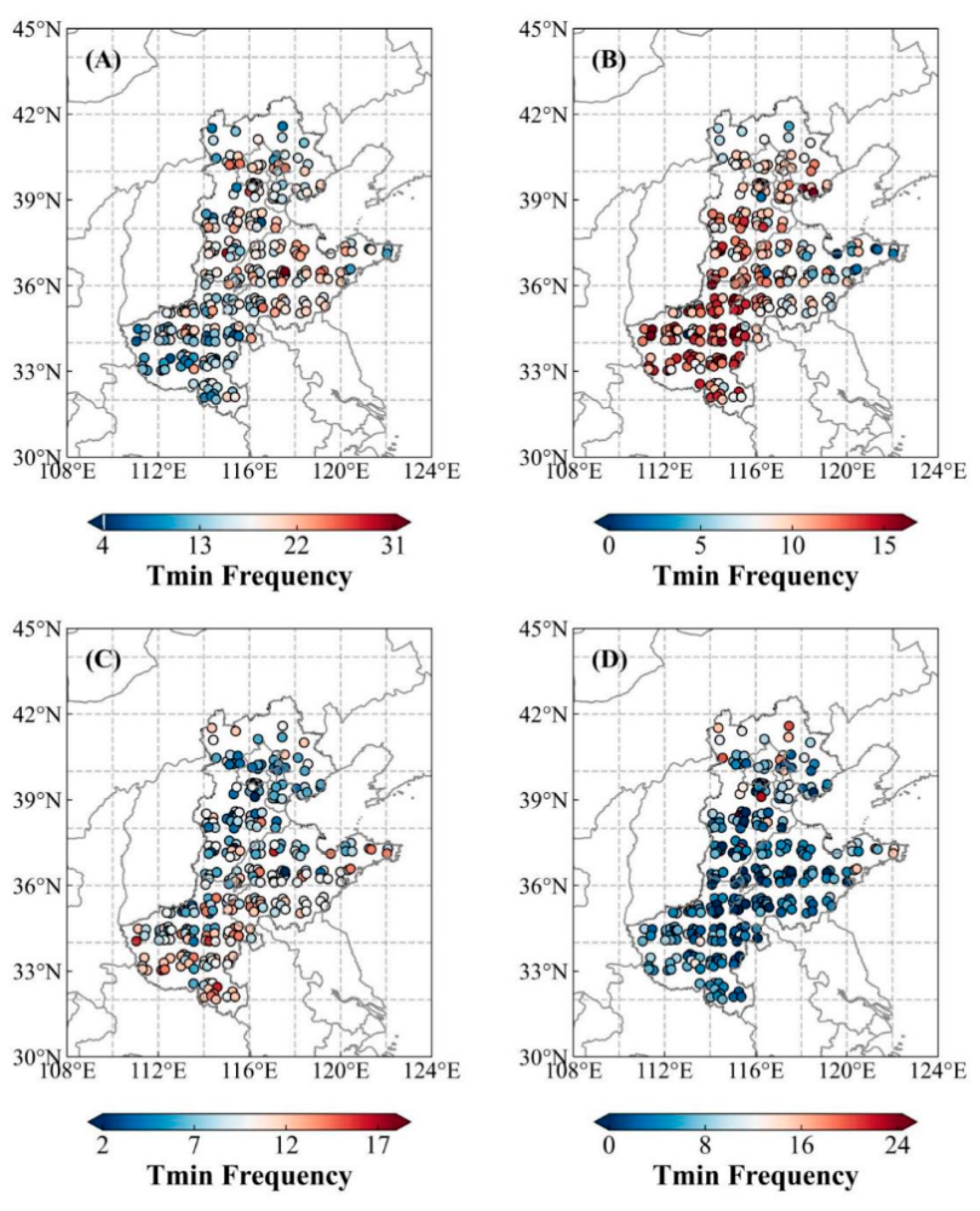
3.2.1. Spatiotemporal Distribution Characteristics of Low-Temperature–Drought Compound Events

Figure 13 depicts the spatial distribution of drought frequency per decade for winter wheat in the 3H Plain from 1982 to 2020. From 1982 to 1991, the regional drought frequency ratio gradually increased from north to south, reaching 40% in western and eastern Shandong and southern Henan. The second highest frequency, 30%, occurred in central and northern Henan and a few areas of Hebei north, while the lowest frequency was 12% in Beijing and central Hebei. From 1992 to 2001, central Henan recorded the highest frequency at 40%. This was followed by 30% in southern Henan, parts of northern Henan, southeastern and northern Shandong, and north Hebei, with the lowest frequency of 10% in Beijing and central Hebei. From 2002 to 2011, eastern Shandong and northern Hebei experienced drought frequencies up to 40%. Southern Henan and central Shandong followed with 30%; the lowest frequencies, at 7%, were in Beijing, Tianjin, and central Hebei. From 2012 to 2020, eastern Shandong and northern Hebei had the highest drought frequency at 37%, while southern Hebei, western Shandong, and north Henan had the lowest, at only 10%. In summary, it has been observed that low-temperature–drought events in the Huang-Huai-Hai Plain have exhibited a regional decreasing trend over the past 39 years.

Figure 14 shows the spatial distribution of the frequency of low temperatures per decade for winter wheat in the Huang-Huai-Hai Plain from 1982 to 2020. From 1982 to 1991, the highest frequency was in central Shandong, at 30%; the second highest was in northern and southern Shandong and central Hebei, at 22%, and the lowest was in central and south Henan, at 7%. From 1992 to 2001, the frequency reached as high as 15% in most of Henan, southern Hebei, and along the border with the Bohai Sea; it was second highest in south Hebei and western Shandong, at 12%, and the lowest in eastern Shandong, at 2%. This period’s minimum temperature events covered most of the Huang-Huai-Hai Plain. From 2002 to 2011, the highest frequency was in southern and western Henan, at 13%; Beijing, central Hebei, and central Shandong had the lowest, at only 4%. From 2012 to 2020, northern Hebei and eastern Shandong had the highest frequency, at 16%, while the other regions had about 5%. Overall, there has been a decreasing trend in the frequency of low-temperature events in the Huang-Huai-Hai Plain over the past 39 years.

Figure 15 depicts the spatial distribution of low-temperature–drought frequency for winter wheat in the 3H Plain for each decade from 1982 to 2020. From 1982 to 1991, the frequency of low-temperature–drought events in central and southern Shandong reached 15%, the highest recorded; Western Henan and southern Hebei followed with 10%, while central Henan recorded the lowest at only 3%. The remaining areas experienced a frequency of approximately 6%. From 1992 to 2001, eastern and northern Henan, along with western Shandong, recorded a low-temperature–drought frequency of 8%; the lowest frequencies, at only 1%, were in Beijing, central and northern Hebei, western and southern Henan, and eastern Shandong. From 2002 to 2011, the highest frequency of low temperature–drought, at 9%, occurred in south and west Henan and southeastern Shandong; the lowest frequencies, at 1%, were found in northern Henan, central and north Hebei, and Beijing and Tianjin. From 2012 to 2020, northern Hebei and eastern Shandong experienced the highest low temperature–drought frequency at 8%; the lowest, at only 1%, was in the entire province of Henan, western Shandong, and southern Hebei. Over the past 39 years, the frequency of low-temperature–drought events has decreased, and the frequency of low-temperature–drought compound events is significantly lower than that of high-temperature–drought events.

According to Figure 16, the proportion of low-temperature–drought compound events to drought events in the 3H Plain significantly decreased from 1982 to 2020, with a reduction rate of 3% per decade, and the interannual fluctuation in this proportion was substantial. In particular, 1983 saw the highest proportion at 85%, followed by 2011 with 80%. No compound events occurred in 1989, 1999, 2001, 2002, 2006, or 2015. On a spatial scale, compound events in central Hebei and western Shandong accounted for the highest proportions, at 22%. Southern Hebei and central Shandong followed at 20%, while central Henan recorded the lowest, at only 8%. Overall, the proportion of low-temperature–drought compound events compared to drought events is significantly lower than that for high temperature–drought, displaying a distribution pattern with lower frequencies in the south and higher frequencies in the north.

Figure 17 illustrates the spatial evolution of low-temperature–drought compound events in the Huang-Huai-Hai Plain from 1982 to 2020. With a 3-month lag, southern Hebei, northern Henan, and western Shandong have the highest positive correlation coefficients at 0.3, while north Hebei has the highest negative correlation at −0.4. With a 2-month lag, northern Henan, Tianjin, and southern Hebei have the highest positive correlation coefficients at 0.4, while a few stations north of Hebei record the highest negative correlation at −0.4. With a 3-month lag, the highest positive correlation between low temperature and the NDVI was 0.5 in western and southern Hebei, while the highest negative correlation was −0.4 in south Henan, west Shandong, and southern Hebei. With a 2-month lag, northern Hebei, Beijing, Tianjin, and northern Shandong had the highest positive correlation at 0.3, while central and south Henan recorded the highest negative correlation at −0.4. With a 1-month lag, Hebei North had the highest positive correlation at 0.5, while Tianjin, Beijing, and southern Henan had the highest negative correlation at −0.3. The highest positive correlation coefficient of −0.3 was found in northern Hebei, Beijing, and Tianjin, and the highest negative correlation coefficient of −0.4 was found in western Shandong and north Henan for the exact monthly correlation between low temperature and the NDVI. Overall, in low-temperature–drought compound events, the NDVI showed a positive correlation with drought and a negative correlation with minimum temperature across most of the 3H Plain.

3.2.2. Sensitivity of Winter Wheat to Low-Temperature–Drought Compound Events

Figure 18 shows the Empirical Cumulative Distribution Function (ECDF) of low-temperature–drought compound events for winter wheat in the typical regions of the Huang-Huai-Hai Plain from 1982 to 2020. As shown in the figure, 80% of the sites experienced low-temperature–drought compound events during the period from 2001 to 2020. For the past 20 years, the ECDF is characterized by a steeply sloped curve, indicating that the data may follow a skewed distribution, and the sites within this interval are more densely clustered, suggesting that the occurrence of compound drought events is relatively concentrated. For the period from 1982 to 2000, the occurrence and distribution patterns of low-temperature–drought compound events were similar to those in the 2001–2020 period. When the proportion of sites experiencing compound events is less than 40%, the ECDF curve is relatively steep, indicating that 40% of the sites are relatively concentrated; when the proportion of sites is between 40% and 80%, the curve is relatively flat, indicating that the occurrence of compound drought events is more dispersed.

Figure 19 shows the sensitivity characteristics of winter wheat in relation to variations in low-temperature–drought compound events using the random forest method, we conducted an attribution analysis and obtained Figure 19. According to the sensitivity identification of climate factors for winter wheat in the Huang-Huai-Hai Plain from 1982 to 2020, it is evident that, in low-temperature–drought compound events, winter wheat shows comparable sensitivity to maximum temperature, minimum temperature, precipitation, and the drought index (SPI), each around 13%. Overall, in both high-temperature–drought and low-temperature–drought compound events, winter wheat exhibits higher sensitivity to extreme temperatures compared to precipitation and the SPI, with a greater sensitivity to high temperatures.

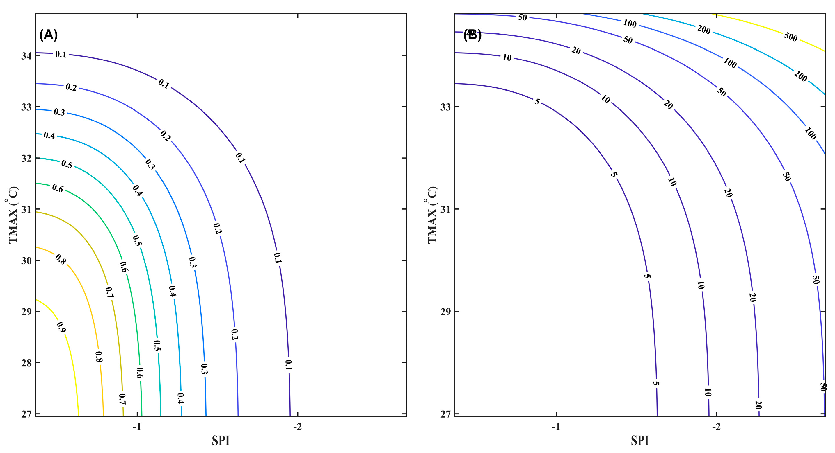
3.2.3. Copula Analysis of Low-Temperature–Drought Compound Events

Table 6. Kendall/Spearman/Pearson rank correlation coefficients for drought (SPI) and extreme low temperature (TMIN) in the 3H Plain, 1982–2020.

Factors Name	Kendall		Spearman		Pearson
	r	p Value	r	p Value	r	p Value
3H Plain _SPI_TMIN	0.148	0.0008	0.172	0.0007	0.149	0.0217

shows that the correlation between drought (SPI) and extreme low temperature (TMIN) in the 3H Plain is positively correlated, passing the 5% significance test. Given the analysis results, modeling the binary distribution of TMIN and the SPI using a copula approach is feasible.

According to

Table 7. Cluster selection criteria of copula function for drought–extreme low temperature in the 3H Plain.

Cop_Family	AIC	BIC	RMSE
Gaussian	18.56	24.26	0.192
t	20.56	31.96	0.194
Clayton	17.96	23.66	0.412
Frank	18.77	24.46	0.175
Gumbel	17.96	23.66	0.412

, for the TMIN-SPI copula function selection for the 3H Plain, the Frank copula approach is identified as optimal across three evaluation metrics—AIC, BIC, and RMSE—showing values for these metrics that are lower than those for the other four copula types. This indicates that the Frank copula type provides the best fit and is most suitable for describing extremely low temperature and SPI joint distribution characteristics. Therefore, this paper selects the Frank copula function to establish a two-dimensional joint probability distribution model for extremely low temperatures and drought in the 3H Plain.

Figure 20 displays the probability distribution function for low-temperature–drought compound events in the 3H Plain from 1982 to 2020. Figure 20A illustrates that the scatter points, representing actual and theoretical frequencies, closely align with the fitted line, demonstrating that their overall trends are consistent, effectively capturing the joint distribution characteristics of the SPI and TMIN. This confirms that the copula model can accurately represent these variables’ joint behaviors. Additionally, it accurately captures the marginal distributions of the SPI and TMIN. From Figure 20B, the probability of low-temperature–drought compound events increases with rising minimum temperatures, and similarly rises as SPI increases (indicating decreasing drought intensity), with more minor fluctuations in event probability when temperatures range from −2 to −6 °C and the SPI ranges from −2 to −1.5.

Figure 21A illustrates the joint probability distribution relationship between drought and extremely low temperature in the 3H Plain. The figure enables the determination of the joint probability of extremely low temperature and drought at any point. This function reflects the correlation between extremely low temperatures and drought across various value ranges. Notably, the figure displays an asymmetric and skewed dependence structure on a monthly scale, with extremely low temperatures exerting minimal impact on drought at low values and significant impact at very high values. One can derive the interval distribution for extreme heat and drought using contour plots with joint probabilities ranging from 0.1 to 0.9. The contour plots show that the joint probability is higher when extremely low temperature is fixed and drought severity is lower, or when drought severity is fixed and the minimum temperature is lower. Significant differences exist in the joint probability of minimum temperature and the SPI across different intervals on the same contour. The figure reveals that scenarios where minimum temperature pairs with both minimum and maximum SPI values exhibit low joint probabilities, except when both are at maximum values, where the probability is high. Additionally, low-temperature–drought compound events are more likely during low-temperature and mild drought periods.

Figure 21B shows the two-dimensional contours of the joint reproduction period of extremely low temperature–SPI in the 3H Plain. The reproduction period corresponding to extremely low temperatures or SPI greater than or equal to a specific value can be calculated using the joint reproduction period plot. The plots reflect combinations of extremely low temperature or SPI greater than or equal to a particular value when the return periods are 2, 5, 10, 25, 50, and 100 years, respectively. The smaller the joint return period, the more extensive the range of values of extreme low temperature and SPI, suggesting that the SPI is more likely to have a smaller return period when extreme low temperature is specific. Low-temperature–drought compound events are more likely to occur during overlapping low-temperature and mild drought periods.

Figure 22A shows the contour plot of the joint probability of exceeding extremely low temperature–SPI in the 3H Plain. According to the figure, when the drought level is fixed, as the minimum temperature decreases, the joint probability of exceeding the low-temperature–drought compound event decreases; similarly, when the minimum temperature is held constant, as the SPI decreases (indicating an increase in drought intensity), the joint probability of exceeding the compound event follows suit. The joint exceedance probability can be obtained from the joint exceedance probability graph when the minimum temperature and the SPI are arbitrary values. The figure displays combinations where the minimum temperature and SPI are simultaneously greater than or equal to specific values, with joint exceedance probabilities ranging from 0.1 to 0.9. The smaller the values of extremely low temperature and the SPI are, the smaller the joint exceeding likelihood is, and vice versa. This comparison implies that smaller values of extremely low temperature and the SPI are more likely to exceed larger ones.

Figure 22B illustrates the co-occurring recurrence periods for extremely low temperatures and drought in the 3H Plain. As can be seen from the figure, when the drought level is fixed, the compound event joint beyond the reproduction period grows as the minimum temperature decreases. In contrast, when the extremely low temperature is fixed, the compound event joint beyond the reproduction period grows as the SPI decreases (drought intensity strengthens). At the same time, the reproduction period is longer when the temperature is lower, and the drought intensity is weaker. The reproduction period for which extremely low temperature and the SPI are greater than or equal to a specific value can be seen from the same exceeding reproduction period plot. The figure shows combinations of extremely low temperature and the SPI at the same time greater than or equal to a specific value for return periods of 2, 5, 10, 25, 50, and 100 years. For cases with extremely low temperature and SPI-fixed values, their coeval return periods are significantly larger than the joint return period. For the synoptic return period, the larger the given return period, the smaller the values of extreme low temperature and SPI, and even the synoptic return period exceeds 100 years when the values of extreme low temperature and drought level are large enough.

4. Discussion

4.1. Impact of High-Temperature–Drought Compound Events

From 1982 to 2020, high-temperature–drought compound events in the 3H Plain demonstrated a north-to-south expansion trend, influenced by climate change, environmental conditions, and human activities [88]. Global warming increases high-temperature events, while regional climate changes make areas more drought-prone [89]. These events significantly impact winter wheat growth, with higher maximum temperatures increasing their probability and potential to limit growth and affect grain yields [90]. Sensitivity analyses reveal that winter wheat is most sensitive to maximum temperature, followed by minimum temperature, precipitation, and the SPI. This indicates that temperature changes more significantly affect growth during heat–drought events than precipitation [91]. These findings highlight the need for disaster prevention and response strategies under high temperatures and mild drought conditions.

Winter wheat is more sensitive to maximum air temperature than to precipitation and the SPI during heat–drought events, likely due to increased evaporation reducing soil moisture [92]. The NDVI is negatively correlated with drought and positively correlated with maximum air temperature, indicating that reduced soil moisture under high temperatures and drought can stunt growth, decreasing NDVI values [93,94]. Conversely, high temperatures can accelerate growth, increasing NDVI values, making the NDVI an effective indicator for monitoring and predicting drought conditions and crop growth in the 3H Plain [95].

4.2. Impact of Low-Temperature–Drought Compound Events

From 1982 to 2020, the frequency of low-temperature–drought compound events in the 3H Plain decreased, significantly more so than high-temperature–drought events. This is likely due to global warming reducing winter low-temperature events and increasing drought susceptibility in northern regions [96]. The impact on winter wheat, especially when minimum temperature and SPI are fixed, should still be considered. The co-occurrence return period for these events is significantly longer than the joint return period, suggesting a higher likelihood of co-occurrence and potentially longer durations than high-temperature–drought events. Longer return periods correspond to lower minimum temperature and SPI values, indicating a decreased likelihood of simultaneous low temperature and drought over time. Winter wheat shows a specific sensitivity pattern to elements of low-temperature–drought compound events. Sensitivity to maximum air temperature exceeds that to minimum air temperature, precipitation, and the SPI, suggesting susceptibility to higher temperatures under low temperatures and drought. Winter wheat is positively correlated with drought and negatively correlated with minimum temperature across most regions [97]. This suggests that, under drought, lower minimum air temperatures adversely affect vegetation growth [98]. As minimum temperatures rise, winter wheat’s sensitivity to low-temperature–drought compound events increases, potentially limiting its growth and impacting grain yields.

Climate change significantly affects low-temperature–drought events. Rising temperatures in recent decades may reduce low-temperature events. Global warming might alter precipitation patterns, impacting drought events’ frequency and duration [99,100]. Located near the Yellow and Bohai Sea, the 3H Plain may experience climate effects due to changes in sea surface temperatures. Anomalies in sea surface temperatures can alter atmospheric circulation, influencing low-temperature and drought events. Atmospheric circulation patterns significantly influence cold-temperature–drought events [101,102]. Low-temperature events are more probable with cold air influxes. Shifts in atmospheric circulation could modify precipitation patterns, affecting drought. Land-use changes could influence low-temperature–drought events [103]. Large-scale agricultural irrigation could alter local temperature and precipitation patterns, impacting low-temperature and drought frequency. Human activities significantly contribute to the occurrence and impacts of low-temperature–drought events [104]. Agricultural practices, water management, and land use may directly or indirectly influence regional climates and drought conditions. The increasing use and demand for natural resources, driven by population growth and economic development, may impact the frequency and severity of cold–drought events.

4.3. Overall Impact of Climate Change on Winter Wheat Growth

The trend of climate change in the 3H Plain coincides with the trend of global warming. Global warming increases surface temperatures, leading to higher maximum air temperatures in the 3H Plain, increasing high-temperature events’ frequency and intensity. Warming might change precipitation patterns, potentially leading to more frequent drought events [105]. These effects interact, increasing heat–drought compound events. Furthermore, changes in maximum and minimum temperatures significantly impact crops. Winter wheat in the 3H Plain is most sensitive to maximum air temperature, indicating the serious impacts of climate warming on growth and yield. Winter wheat negatively correlates with drought and positively correlates with maximum air temperature, suggesting that rising temperatures could affect vegetation growth and increase drought risk.

Under global warming, high-temperature weather frequency increases, driving more compound extreme-heat and drought events. Weather systems greatly influence high temperatures; conditions favoring high temperatures often disfavor precipitation, closely correlating high temperatures and drought [13]. Even with stable drought frequency, rising high temperatures will increase compound extreme heat and drought events [16], consistent with this study’s conclusions.

4.4. Agricultural Adaptation Strategies

Policies, technologies, and socio-economic conditions can influence the ability to cope with high temperatures and droughts in the 3H Plain. Recent compound drought events in the 3H Plain have posed severe challenges to water resources, causing groundwater decline and water scarcity, and affecting ecosystems and social stability. Recommendations for addressing drought resistance and disaster reduction in the 3H Plain include the following:

(1)

Develop water-saving projects and advanced irrigation technologies like drip and sprinkler irrigation. Promote drought-resistant crop varieties.

(2)

Conserve water in industrial and residential areas by optimizing processes and increasing public awareness.

(3)

Improve water conservancy projects, including reservoirs, irrigation channels, and rainwater collection systems. Enhance drought resistance management and scientific research.

(4)

Rationally allocate water resources, consider inter-basin transfers, and prioritize domestic and agricultural water use in scarce areas.

(5)

Maintain soil moisture by using mulch, such as straw or plastic film, to cover the soil surface and reduce evaporation. Deep tillage can also help maintain soil moisture by increasing soil porosity and enhancing the soil’s water retention capacity.

(6)

Plant drought-resistant crops; optimize planting schedules by adjusting planting and harvesting times based on climatic conditions to avoid crop growth during drought periods, thereby reducing water demand.

To address climate change challenges and achieve climate-smart agriculture, applying climate-resistant wheat varieties is essential. Extreme climatic events, such as high temperatures and droughts, significantly impact winter wheat growth and yield [106]. Promoting climate-resistant varieties enhances agricultural stability and sustainability, ensuring high yield and quality under extreme conditions and thus securing food supply. Selection methods combine traditional breeding and modern biotechnology. Hybrid breeding and gene editing can identify and accelerate the development of resistant varieties. Multi-environment trials under different climatic conditions help evaluate and identify the most adaptable varieties.

Integrating climate and crop growth data with machine learning can predict promising climate-resistant wheat varieties. Agricultural extension services can promote these varieties to farmers and provide planting guidance. Supporting farmers in cultivating these varieties enhances resistance to extreme climatic events and improves agricultural resilience, achieving sustainable development. These research directions provide crucial scientific and technical support for future climate change challenges.

Future research will focus on the following aspects:

(1)

Improving time series analysis models: Future research will integrate deep learning models like CNN, RNN, and LSTM to better capture spatiotemporal changes in climate data and improve the accuracy of climate event analysis. Ensemble learning methods will enhance model robustness and stability, providing reliable tools for analyzing historical climate events and supporting agricultural adaptation strategies.

(2)

Expanding research areas and time frames: Future research will expand the study area to a national or global scope and extend the time frame to include more years of data. Integrating the latest meteorological and remote sensing data will improve the accuracy and comprehensiveness of the research, helping to identify long-term climate change trends and their impacts on agricultural production.

(3)

Comprehensive multi-factor analysis: Future research will include other climatic factors such as precipitation, wind speed, and humidity to assess their combined effects on winter wheat growth. Multivariate time series models will analyze the interactions among these factors, enabling more accurate predictions of winter wheat growth under varying climatic conditions.

5. Conclusions

In this paper, the sensitivity of winter wheat to extreme temperature–drought compound events is investigated by analyzing the spatial and temporal distribution characteristics of high- and low-temperature–drought compound events. These compound events’ probability distribution and occurrence patterns across different recurrence periods are analyzed using copula analysis to explore winter wheat’s response to high- and low-temperature–drought compound events. The main conclusions are as follows:

(1)

Temporal and spatial distribution characteristics of high-temperature–drought compound events.

From 1982 to 2020, the spatial distribution of high-temperature and drought events in the 3H Plain displayed an expanding trend, particularly noted by the southward expansion of drought-affected areas. During this period, the frequency of high-temperature events also showed an overall increasing trend, further indicating the apparent impact of climate change. From 2001 to 2020, about 40% of the observation stations experienced high-temperature–drought compound events, and the occurrence areas of these compound events were relatively concentrated. During 1982–2000, about 60% of the stations experienced such compound events, showing changes in the frequency and distribution area of compound events in different periods.

(2)

Sensitivity of winter wheat to high-temperature–drought compound events.

In high-temperature–drought compound events, winter wheat’s sensitivity to climatic elements is ranked as follows: maximum temperature > minimum temperature > precipitation > SPI. This highlights maximum temperature as the critical factor influencing growth. The NDVI was negatively correlated with drought and positively correlated with maximum air temperature in most areas. This finding highlights the crucial role of maximum air temperature on winter wheat growth and climate change’s impact on agroecosystems.

(3)

Recurrence period of combined heat–drought events.

The copula analysis of high-temperature–drought compound events indicated that maximum air temperature and SPI increase the likelihood of these compound events occurring. In addition, the changes in the probability of compound events were more stable when the temperature was 28–30 °C and when the SPI was from −2 to −2.5, indicating that the effects of compound events were more pronounced under these conditions. High-temperature–drought compound events were more likely to occur under high-temperature and mild drought conditions. This is further confirmed by the analysis of the joint exceedance probability and return period, pointing to an increased chance of occurrence of such compound events at certain temperatures and drought levels.

(4)

Temporal and spatial distribution characteristics of low-temperature–drought compound events.

Between 1982 and 2020, there was a general decline in the frequency of low-temperature events in the 3H Plain. At the same time, the frequency of low-temperature–drought compound events also showed a decreasing trend, which was significantly lower than the frequency of high-temperature–drought compound events. The proportion of low-temperature–drought compound events relative to total drought events was small, with a geographic pattern of lower occurrence in the south and higher occurrence in the north. During the period of 2001–2020, about 80% of the stations recorded low-temperature–drought compound events, and the regions in which the events occurred were relatively concentrated, whereas, during the period of 1982–2000, the proportion ranged from 40% to 80%. The areas in which the events occurred were more dispersed.

(5)

Sensitivity of winter wheat to low-temperature–drought compound events.

In low-temperature–drought compound events, the sensitivity of winter wheat to meteorological elements was ranked as follows: maximum temperature > minimum temperature > precipitation > SPI. In addition, the NDVI was positively correlated with drought and negatively correlated with minimum temperature in most areas, indicating that the growth of winter wheat was significantly affected by low-temperature conditions.

(6)

Recurrence period of low-temperature–drought compound events.

The copula analysis results for the low-temperature–drought compound events revealed that an increase in minimum air temperature and the SPI heightened the probability of these compound events. Especially when the minimum temperature is −2 to −6 °C and the SPI is −2 to −1.5, the change in the likelihood of occurrence of the compound event is more stable. Low-temperature–drought compound events were more likely to occur under low-temperature and mild drought conditions. For fixed values of minimum temperature and SPI, the synoptic return period of compound events is significantly larger than the joint return period, and the longer the return period, the smaller the values of minimum temperature and SPI, reflecting the relationship between the probability of occurrence of this type of compound event and the return period.

This study reveals that, from 1982 to 2020, high-temperature–drought events in the Huang-Huai-Hai Plain increased in frequency and intensity, reducing wheat yields by 15–20%. Low-temperature drought events, although less frequent, still caused a 10–15% yield reduction. The drought index during the winter wheat-growing season has risen, increasing the impact of drought on yield loss. Copula analysis effectively assesses and predicts these events, highlighting the need for adaptation and mitigation strategies to protect agricultural production from climate change. This research provides a scientific basis for understanding climate change impacts on agroecosystems and guides the development of adaptive responses.

References

1. Manning, C.; Widmann, M.; Bevacqua, E.; Van Loon, A.F.; Maraun, D.; Vrac, M. Increased probability of compound long-duration dry and hot events in Europe during summer (1950–2013). Environ. Res. Lett. 2019, 14, 094006. [Google Scholar] [CrossRef]
2. Cook, B.I.; Mankin, J.S.; Anchukaitis, K.J. Climate Change and Drought: From Past to Future. Curr. Clim. Chang. Rep. 2018, 4, 164–179. [Google Scholar] [CrossRef]
3. Bektaş, Y.; Sakarya, A. The Relationship between the Built Environment and Climate Change: The Case of Turkish Provinces. Sustainability 2023, 15, 1659. [Google Scholar] [CrossRef]
4. Alonso, L.; Renard, F. A Comparative Study of the Physiological and Socio-Economic Vulnerabilities to Heat Waves of the Population of the Metropolis of Lyon (France) in a Climate Change Context. Int. J. Environ. Res. Public Health 2020, 17, 1004. [Google Scholar] [CrossRef] [PubMed]
5. Yu, R.; Zhai, P. More frequent and widespread persistent compound drought and heat event observed in China. Sci. Rep. 2020, 10, 14576. [Google Scholar] [CrossRef] [PubMed]
6. Potopová, V.; Lhotka, O.; Možný, M.; Musiolková, M. Vulnerability of hop-yields due to compound drought and heat events over European key-hop regions. Int. J. Climatol. 2021, 41, E2136–E2158. [Google Scholar] [CrossRef]
7. Han, H.; Jian, H.; Liu, M.; Lei, S.; Yao, S.; Yan, F. Impacts of drought and heat events on vegetative growth in a typical humid zone of the middle and lower reaches of the Yangtze River, China. J. Hydrol. 2023, 620, 129452. [Google Scholar] [CrossRef]
8. Ye, L.; Shi, K.; Xin, Z.; Wang, C.; Zhang, C. Compound Droughts and Heat Waves in China. Sustainability 2019, 11, 3270. [Google Scholar] [CrossRef]
9. Martius, O.; Pfahl, S.; Chevalier, C. A global quantification of compound precipitation and wind extremes. Geophys. Res. Lett. 2016, 43, 7709–7717. [Google Scholar] [CrossRef]
10. Abdin, A.F.; Fang, Y.P.; Zio, E. A modeling and optimization framework for power systems design with operational flexibility and resilience against extreme heat waves and drought events. Renew. Sustain. Energy Rev. 2019, 112, 706–719. [Google Scholar] [CrossRef]
11. Bezak, N.; Mikoš, M. Changes in the Compound Drought and Extreme Heat Occurrence in the 1961–2018 Period at the European Scale. Water 2020, 12, 3543. [Google Scholar] [CrossRef]
12. Vogel, M.M.; Zscheischler, J.; Wartenburger, R.; Dee, D.; Seneviratne, S.I. Concurrent 2018 Hot Extremes Across Northern Hemisphere Due to Human-Induced Climate Change. Earth’s Future 2019, 7, 692–703. [Google Scholar] [CrossRef] [PubMed]
13. Zscheischler, J.; Seneviratne, S.I. Dependence of drivers affects risks associated with compound events. Sci. Adv. 2017, 3, e1700263. [Google Scholar] [CrossRef] [PubMed]
14. Bastos, A.; Ciais, P.; Friedlingstein, P.; Sitch, S.; Pongratz, J.; Fan, L.; Wigneron, J.P.; Weber, U.; Reichstein, M.; Fu, Z.; et al. Direct and seasonal legacy effects of the 2018 heat wave and drought on European ecosystem productivity. Sci. Adv. 2020, 6, eaba2724. [Google Scholar] [CrossRef] [PubMed]
15. Alizadeh, M.R.; Adamowski, J.; Nikoo, M.R.; AghaKouchak, A.; Dennison, P.; Sadegh, M. A century of observations reveals increasing likelihood of continental-scale compound dry-hot extremes. Sci. Adv. 2020, 6, eaaz4571. [Google Scholar] [CrossRef] [PubMed]
16. Yu, R.; Zhai, P. Changes in compound drought and hot extreme events in summer over populated eastern China. Weather Clim. Extrem. 2020, 30, 100295. [Google Scholar] [CrossRef]
17. Van Vuuren, D.P.; Riahi, K.; Moss, R.; Edmonds, J.; Thomson, A.; Nakicenovic, N.; Kram, T.; Berkhout, F.; Swart, R.; Janetos, A.; et al. A proposal for a new scenario framework to support research and assessment in different climate research communities. Glob. Environ. Chang. 2012, 22, 21–35. [Google Scholar] [CrossRef]
18. Mazdiyasni, O.; AghaKouchak, A. Substantial increase in concurrent droughts and heatwaves in the United States. Proc. Natl. Acad. Sci. USA 2015, 112, 11484–11489. [Google Scholar] [CrossRef] [PubMed]
19. Russo, A.; Gouveia, C.M.; Dutra, E.; Soares, P.M.M.; Trigo, R.M. The synergy between drought and extremely hot summers in the Mediterranean. Environ. Res. Lett. 2019, 14, 014011. [Google Scholar] [CrossRef]
20. Sharma, S.; Mujumdar, P. Increasing frequency and spatial extent of concurrent meteorological droughts and heatwaves in India. Sci. Rep. 2017, 7, 15582. [Google Scholar] [CrossRef]
21. Lu, Y.; Hu, H.; Li, C.; Tian, F. Increasing compound events of extreme hot and dry days during growing seasons of wheat and maize in China. Sci Rep 2018, 8, 16700. [Google Scholar] [CrossRef] [PubMed]
22. Dosio, A.; Mentaschi, L.; Fischer, E.; Wyser, K. Extreme heat waves under 1.5 °C and 2 °C global warming. Environ. Res. Lett. 2018, 13, 054006. [Google Scholar] [CrossRef]
23. Gasparrini, A.; Guo, Y.; Sera, F.; Vicedo-Cabrera, A.M.; Huber, V.; Tong, S.; de Sousa Zanotti Stagliorio Coelho, M.; Nascimento Saldiva, P.H.; Lavigne, E.; Matus Correa, P.; et al. Projections of temperature-related excess mortality under climate change scenarios. Lancet Planet. Health 2017, 1, e360–e367. [Google Scholar] [CrossRef] [PubMed]
24. Zscheischler, J.; Westra, S.; van den Hurk, B.J.J.M.; Seneviratne, S.I.; Ward, P.J.; Pitman, A.; AghaKouchak, A.; Bresch, D.N.; Leonard, M.; Wahl, T.; et al. Future climate risk from compound events. Nat. Clim. Chang. 2018, 8, 469–477. [Google Scholar] [CrossRef]
25. Zscheischler, J.; Martius, O.; Westra, S.; Bevacqua, E.; Raymond, C.; Horton, R.M.; van den Hurk, B.; AghaKouchak, A.; Jézéquel, A.; Mahecha, M.D.; et al. A typology of compound weather and climate events. Nat. Rev. Earth Environ. 2020, 1, 333–347. [Google Scholar] [CrossRef]
26. Bevacqua, E.; Maraun, D.; Hobæk Haff, I.; Widmann, M.; Vrac, M. Multivariate statistical modelling of compound events via pair-copula constructions: Analysis of floods in Ravenna (Italy). Hydrol. Earth Syst. Sci. 2017, 21, 2701–2723. [Google Scholar] [CrossRef]
27. Leonard, M.; Westra, S.; Phatak, A.; Lambert, M.; van den Hurk, B.; McInnes, K.; Risbey, J.; Schuster, S.; Jakob, D.; Stafford-Smith, M. A compound event framework for understanding extreme impacts. WIREs Clim. Chang. 2014, 5, 113–128. [Google Scholar] [CrossRef]
28. Mohammed, S.; Alsafadi, K.; Enaruvbe, G.O.; Bashir, B.; Elbeltagi, A.; Széles, A.; Alsalman, A.; Harsanyi, E. Assessing the impacts of agricultural drought (SPI/SPEI) on maize and wheat yields across Hungary. Sci. Rep. 2022, 12, 8838. [Google Scholar] [CrossRef] [PubMed]
29. Liu, C.; Yang, C.; Yang, Q.; Wang, J. Spatiotemporal drought analysis by the standardized precipitation index (SPI) and standardized precipitation evapotranspiration index (SPEI) in Sichuan Province, China. Sci. Rep. 2021, 11, 1280. [Google Scholar] [CrossRef]
30. Wang, Q.; Zeng, J.; Qi, J.; Zhang, X.; Zeng, Y.; Shui, W.; Xu, Z.; Zhang, R.; Wu, X.; Cong, J. A multi-scale daily SPEI dataset for drought characterization at observation stations over mainland China from 1961 to 2018. Earth Syst. Sci. Data 2021, 13, 331–341. [Google Scholar] [CrossRef]
31. Pei, Z.; Fang, S.; Wang, L.; Yang, W. Comparative Analysis of Drought Indicated by the SPI and SPEI at Various Timescales in Inner Mongolia, China. Water 2020, 12, 1925. [Google Scholar] [CrossRef]
32. Wang, Z.; Yang, Y.; Zhang, C.; Hui, G.; Hou, Y. Historical and future Palmer Drought Severity Index with improved hydrological modeling. J. Hydrol. 2022, 610, 127941. [Google Scholar] [CrossRef]
33. Chen, L.; Chen, X.; Cheng, L.; Zhou, P.; Liu, Z. Compound hot droughts over China: Identification, risk patterns and variations. Atmos. Res. 2019, 227, 210–219. [Google Scholar] [CrossRef]
34. Hao, Z.; Hao, F.; Singh, V.; Zhang, X. Quantifying the relationship between compound dry and hot events and El Niño–Southern Oscillation (ENSO) at the global scale. J. Hydrol. 2018, 567, 332–338. [Google Scholar] [CrossRef]
35. Olmo, M.; Bettolli, M.L.; Rusticucci, M. Atmospheric circulation influence on temperature and precipitation individual and compound daily extreme events: Spatial variability and trends over southern South America. Weather Clim. Extrem. 2020, 29, 100267. [Google Scholar] [CrossRef]
36. Geirinhas, J.L.; Russo, A.; Libonati, R.; Sousa, P.M.; Miralles, D.G.; Trigo, R.M. Recent increasing frequency of compound summer drought and heatwaves in Southeast Brazil. Environ. Res. Lett. 2021, 16, 034036. [Google Scholar] [CrossRef]
37. Li, K.; Wang, M.; Liu, K. The Study on Compound Drought and Heatwave Events in China Using Complex Networks. Sustainability 2021, 13, 12774. [Google Scholar] [CrossRef]
38. Muthuvel, D.; Mahesha, A. Spatiotemporal Analysis of Compound Agrometeorological Drought and Hot Events in India Using a Standardized Index. J. Hydrol. Eng. 2021, 26, 04021022. [Google Scholar] [CrossRef]
39. Kang, Y.; Guo, E.; Wang, Y.; Bao, Y.; Bao, Y.; Mandula, N.; Runa, A.; Gu, X.; Jin, L. Characterisation of compound dry and hot events in Inner Mongolia and their relationship with large-scale circulation patterns. J. Hydrol. 2022, 612, 128296. [Google Scholar] [CrossRef]
40. Wu, X.; Hao, Z.; Hao, F.; Singh, V.P.; Zhang, X. Dry-hot magnitude index: A joint indicator for compound event analysis. Environ. Res. Lett. 2019, 14, 064017. [Google Scholar] [CrossRef]
41. Wu, X.; Hao, Z.; Zhang, X.; Li, C.; Hao, F. Evaluation of severity changes of compound dry and hot events in China based on a multivariate multi-index approach. J. Hydrol. 2020, 583, 124580. [Google Scholar] [CrossRef]
42. Wu, X.; Hao, Z.; Hao, F.; Zhang, X. Variations of compound precipitation and temperature extremes in China during 1961–2014. Sci. Total Environ. 2019, 663, 731–737. [Google Scholar] [CrossRef] [PubMed]
43. Miralles, D.G.; Gentine, P.; Seneviratne, S.I.; Teuling, A.J. Land-atmospheric feedbacks during droughts and heatwaves: State of the science and current challenges. Ann. N. Y. Acad. Sci. 2019, 1436, 19–35. [Google Scholar] [CrossRef]
44. AghaKouchak, A.; Cheng, L.; Mazdiyasni, O.; Farahmand, A. Global warming and changes in risk of concurrent climate extremes: Insights from the 2014 California drought. Geophys. Res. Lett. 2014, 41, 8847–8852. [Google Scholar] [CrossRef]
45. Dirmeyer, P.A.; Jin, Y.; Singh, B.; Yan, X. Evolving Land–Atmosphere Interactions over North America from CMIP5 Simulations. J. Clim. 2013, 26, 7313–7327. [Google Scholar] [CrossRef]
46. van den Hurk, B.; van Meijgaard, E.; de Valk, P.; van Heeringen, K.-J.; Gooijer, J. Analysis of a compounding surge and precipitation event in the Netherlands. Environ. Res. Lett. 2015, 10, 035001. [Google Scholar] [CrossRef]
47. Hao, Z.; Singh, V.P.; Hao, F. Compound Extremes in Hydroclimatology: A Review. Water 2018, 10, 718. [Google Scholar] [CrossRef]
48. Zhou, S.; Zhang, Y.; Park Williams, A.; Gentine, P. Projected increases in intensity, frequency, and terrestrial carbon costs of compound drought and aridity events. Sci. Adv. 2019, 5, eaau5740. [Google Scholar] [CrossRef] [PubMed]
49. Miao, C.; Qiaohong, S.; Duan, Q.; Wang, Y. Joint analysis of changes in temperature and precipitation on the Loess Plateau during the period 1961–2011. Clim. Dyn. 2016, 47, 3221–3234. [Google Scholar] [CrossRef]
50. Leng, G.; Tang, Q.; Huang, S.; Zhang, X.; Cao, J. Assessments of joint hydrological extreme risks in a warming climate in China. Int. J. Climatol. 2016, 36, 1632–1642. [Google Scholar] [CrossRef]
51. Sillmann, J.; Kharin, V.V.; Zwiers, F.W.; Zhang, X.; Bronaugh, D. Climate extremes indices in the CMIP5 multimodel ensemble: Part 2. Future climate projections. J. Geophys. Res. Atmos. 2013, 118, 2473–2493. [Google Scholar] [CrossRef]
52. Gallant, A.J.E.; Karoly, D.J.; Gleason, K.L. Consistent Trends in a Modified Climate Extremes Index in the United States, Europe, and Australia. J. Clim. 2014, 27, 1379–1394. [Google Scholar] [CrossRef]
53. Ford, T.W.; Quiring, S.M. In situ soil moisture coupled with extreme temperatures: A study based on the Oklahoma Mesonet. Geophys. Res. Lett. 2014, 41, 4727–4734. [Google Scholar] [CrossRef]
54. Hao, Z.; Hao, F.; Singh, V.P.; Ouyang, W.; Zhang, X.; Zhang, S. A joint extreme index for compound droughts and hot extremes. Theor. Appl. Climatol. 2020, 142, 321–328. [Google Scholar] [CrossRef]
55. Ribeiro, A.F.S.; Russo, A.; Gouveia, C.M.; Pires, C.A.L. Drought-related hot summers: A joint probability analysis in the Iberian Peninsula. Weather Clim. Extrem. 2020, 30, 100279. [Google Scholar] [CrossRef]
56. Feng, S.; Hao, Z.; Zhang, X.; Hao, F. Probabilistic evaluation of the impact of compound dry-hot events on global maize yields. Sci. Total Environ. 2019, 689, 1228–1234. [Google Scholar] [CrossRef] [PubMed]
57. Batibeniz, F.; Ashfaq, M.; Diffenbaugh, N.S.; Key, K.; Evans, K.J.; Turuncoglu, U.U.; Önol, B. Doubling of U.S. Population Exposure to Climate Extremes by 2050. Earth’s Future 2020, 8, e2019EF001421. [Google Scholar] [CrossRef]
58. Lavaysse, C.; Naumann, G.; Alfieri, L.; Salamon, P.; Vogt, J. Predictability of the European heat and cold waves. Clim. Dyn. 2019, 52, 2481–2495. [Google Scholar] [CrossRef]
59. Sutanto, S.J.; Vitolo, C.; Di Napoli, C.; D’Andrea, M.; Van Lanen, H.A.J. Heatwaves, droughts, and fires: Exploring compound and cascading dry hazards at the pan-European scale. Environ. Int. 2020, 134, 105276. [Google Scholar] [CrossRef]
60. Carmona, R.; Díaz, J.; Mirón, I.J.; Ortíz, C.; León, I.; Linares, C. Geographical variation in relative risks associated with cold waves in Spain: The need for a cold wave prevention plan. Environ. Int. 2016, 88, 103–111. [Google Scholar] [CrossRef]
61. Smith, E.T.; Sheridan, S.C. The influence of extreme cold events on mortality in the United States. Sci. Total Environ. 2019, 647, 342–351. [Google Scholar] [CrossRef] [PubMed]
62. Liu, J.; Hansen, A.; Varghese, B.; Liu, Z.; Tong, M.; Qiu, H.; Tian, L.; Lau, K.K.-L.; Ng, E.; Ren, C.; et al. Cause-specific mortality attributable to cold and hot ambient temperatures in Hong Kong: A time-series study, 2006–2016. Sustain. Cities Soc. 2020, 57, 102131. [Google Scholar] [CrossRef]
63. Qian, C.; Wang, J.; Dong, S.; Yin, H.; Burke, C.; Ciavarella, A.; Dong, B.; Freychet, N.; Lott, F.C.; Tett, S.F.B. Human Influence on the Record-breaking Cold Event in January of 2016 in Eastern China. Bull. Am. Meteorol. Soc. 2018, 99, S118–S122. [Google Scholar] [CrossRef]
64. Sutanto, S.J.; van der Weert, M.; Wanders, N.; Blauhut, V.; Van Lanen, H.A.J. Moving from drought hazard to impact forecasts. Nat. Commun. 2019, 10, 4945. [Google Scholar] [CrossRef] [PubMed]
65. Wang, P.; Qiao, W.; Wang, Y.; Cao, S.; Zhang, Y. Urban drought vulnerability assessment—A framework to integrate socio-economic, physical, and policy index in a vulnerability contribution analysis. Sustain. Cities Soc. 2020, 54, 102004. [Google Scholar] [CrossRef]
66. Piticar, A.; Croitoru, A.-E.; Ciupertea, F.-A.; Harpa, G.-V. Recent changes in heat waves and cold waves detected based on excess heat factor and excess cold factor in Romania. Int. J. Climatol. 2018, 38, 1777–1793. [Google Scholar] [CrossRef]
67. Tao, F.; Zhang, Z.; Zhang, S.; Rötter, R.P. Heat stress impacts on wheat growth and yield were reduced in the Huang-Huai-Hai Plain of China in the past three decades. Eur. J. Agron. 2015, 71, 44–52. [Google Scholar] [CrossRef]
68. Liu, B.; Liu, L.; Tian, L.; Cao, W.; Zhu, Y.; Asseng, S. Post-heading heat stress and yield impact in winter wheat of China. Glob. Change Biol. 2014, 20, 372–381. [Google Scholar] [CrossRef] [PubMed]
69. Xiao, L.; Liu, L.; Asseng, S.; Xia, Y.; Tang, L.; Liu, B.; Cao, W.; Zhu, Y. Estimating spring frost and its impact on yield across winter wheat in China. Agric. For. Meteorol. 2018, 260–261, 154–164. [Google Scholar] [CrossRef]
70. Chen, Y.; Donohue, R.J.; McVicar, T.R.; Waldner, F.; Mata, G.; Ota, N.; Houshmandfar, A.; Dayal, K.; Lawes, R.A. Nationwide crop yield estimation based on photosynthesis and meteorological stress indices. Agric. For. Meteorol. 2020, 284, 107872. [Google Scholar] [CrossRef]
71. Li, F.; Chen, J.; Zheng, J. Joint forcing of climate warming and ENSO on a dual-cropping system. Agric. For. Meteorol. 2019, 269–270, 10–18. [Google Scholar] [CrossRef]
72. Ren, S.; Guo, B.; Wu, X.; Zhang, L.; Ji, M.; Wang, J. Winter wheat planted area monitoring and yield modeling using MODIS data in the Huang-Huai-Hai Plain, China. Comput. Electron. Agric. 2021, 182, 106049. [Google Scholar] [CrossRef]
73. Zheng, X.; Yu, Z.; Yu, F.; Shi, Y. Grain-filling characteristics and yield formation of wheat in two different soil fertility fields in the Huang–Huai–Hai Plain. Front. Plant Sci. 2022, 13, 932821. [Google Scholar] [CrossRef] [PubMed]
74. Yue, Y.; Yang, W.; Wang, L. Assessment of drought risk for winter wheat on the Huanghuaihai Plain under climate change using an EPIC model-based approach. Int. J. Digit. Earth 2022, 15, 690–711. [Google Scholar] [CrossRef]
75. Liu, Q.; Zhang, G.; Ali, S.; Wang, X.; Wang, G.; Pan, Z.; Zhang, J. SPI-based drought simulation and prediction using ARMA-GARCH model. Appl. Math. Comput. 2019, 355, 96–107. [Google Scholar] [CrossRef]
76. Tao, Y.; Huang, W.; Gan, W.; Shen, H. Research on Ndvi Normalization Method Based on Gf Images. ISPRS Ann. Photogramm. Remote Sens. Spat. Inf. Sci. 2022, 3, 209–215. [Google Scholar] [CrossRef]
77. Rüschendorf, L. Copulas, Sklar’s Theorem, and Distributional Transform. In Mathematical Risk Analysis: Dependence, Risk Bounds, Optimal Allocations and Portfolios; Rüschendorf, L., Ed.; Springer: Berlin/Heidelberg, Germany, 2013; pp. 3–34. [Google Scholar] [CrossRef]
78. Li, H.; Xiong, L.; Jiang, X. Differentially Private Synthesization of Multi-Dimensional Data using Copula Functions. Adv. Database Technol. 2014, 2014, 475–486. [Google Scholar]
79. Al-babtain, A.; Elbatal, I.; Yousof, H.M. A New Flexible Three-Parameter Model: Properties, Clayton Copula, and Modeling Real Data. Symmetry 2020, 12, 440. [Google Scholar] [CrossRef]
80. Chen, J.; Mao, C.; Liu, Z.; Ma, C.; Sha, G.; Duan, Q.; Fan, H.; Qiu, S.; Wang, D. Stochastic planning of integrated energy system based on correlation scenario generation method via Copula function considering multiple uncertainties in renewable energy sources and demands. IET Renew. Power Gener. 2023, 17, 2978–2996. [Google Scholar] [CrossRef]
81. Solea, E.; Li, B. Copula Gaussian Graphical Models for Functional Data. J. Am. Stat. Assoc. 2022, 117, 781–793. [Google Scholar] [CrossRef]
82. Ota, S.; Kimura, M. Effective estimation algorithm for parameters of multivariate Farlie–Gumbel–Morgenstern copula. Jpn. J. Stat. Data Sci. 2021, 4, 1049–1078. [Google Scholar] [CrossRef]
83. Zhang, W.; He, X.; Hamori, S. Volatility spillover and investment strategies among sustainability-related financial indexes: Evidence from the DCC-GARCH-based dynamic connectedness and DCC-GARCH t-copula approach. Int. Rev. Financ. Anal. 2022, 83, 102223. [Google Scholar] [CrossRef]
84. Da Rocha Júnior, R.L.; dos Santos Silva, F.D.; Costa, R.L.; Gomes, H.B.; Pinto, D.D.; Herdies, D.L. Bivariate Assessment of Drought Return Periods and Frequency in Brazilian Northeast Using Joint Distribution by Copula Method. Geosciences 2020, 10, 135. [Google Scholar] [CrossRef]
85. Poonia, V.; Jha, S.; Goyal, M.K. Copula based analysis of meteorological, hydrological and agricultural drought characteristics across Indian river basins. Int. J. Climatol. 2021, 41, 4637–4652. [Google Scholar] [CrossRef]
86. Nabaei, S.; Sharafati, A.; Yaseen, Z.M.; Shahid, S. Copula based assessment of meteorological drought characteristics: Regional investigation of Iran. Agric. For. Meteorol. 2019, 276–277, 107611. [Google Scholar] [CrossRef]
87. Shiau, J. Fitting Drought Duration and Severity with Two-Dimensional Copulas. Water Resour. Manag. 2006, 20, 795–815. [Google Scholar] [CrossRef]
88. Wang, F.; Wang, Y.; Zhang, K.; Hu, M.; Weng, Q.; Zhang, H. Spatial heterogeneity modeling of water quality based on random forest regression and model interpretation. Environ. Res. 2021, 202, 111660. [Google Scholar] [CrossRef]
89. Mukherjee, S.; Mishra, A.; Trenberth, K.E. Climate Change and Drought: A Perspective on Drought Indices. Curr. Clim. Chang. Rep. 2018, 4, 145–163. [Google Scholar] [CrossRef]
90. Yu, H.; Zhang, Q.; Sun, P.; Song, C. Impact of Droughts on Winter Wheat Yield in Different Growth Stages during 2001–2016 in Eastern China. Int. J. Disaster Risk Sci. 2018, 9, 376–391. [Google Scholar] [CrossRef]
91. Asseng, S.; Foster, I.A.N.; Turner, N.C. The impact of temperature variability on wheat yields. Glob. Chang. Biol. 2011, 17, 997–1012. [Google Scholar] [CrossRef]
92. Gu, L.; Chen, J.; Yin, J.; Xu, C.-Y.; Zhou, J. Responses of Precipitation and Runoff to Climate Warming and Implications for Future Drought Changes in China. Earth’s Future 2020, 8, e2020EF001718. [Google Scholar] [CrossRef]
93. Sun, D.; Kafatos, M. Note on the NDVI-LST relationship and the use of temperature-related drought indices over North America. Geophys. Res. Lett. 2007, 34. [Google Scholar] [CrossRef]
94. Luo, H.; Wang, L.; Fang, J.; Li, Y.; Li, H.; Dai, S. NDVI, Temperature and Precipitation Variables and Their Relationships in Hainan Island from 2001 to 2014 Based on MODIS NDVI. In Geo-Informatics in Resource Management and Sustainable Ecosystem: Proceedings of the Third International Conference, GRMSE 2015, Wuhan, China, 16–18 October 2015; Springer: Berlin/Heidelberg, Germany, 2016; pp. 336–344. [Google Scholar]
95. Ichii, K.; Kawabata, A.; Yamaguchi, Y. Global correlation analysis for NDVI and climatic variables and NDVI trends: 1982–1990. Int. J. Remote Sens. 2002, 23, 3873–3878. [Google Scholar] [CrossRef]
96. Humphrey, V.; Berg, A.; Ciais, P.; Gentine, P.; Jung, M.; Reichstein, M.; Seneviratne, S.I.; Frankenberg, C. Soil moisture–atmosphere feedback dominates land carbon uptake variability. Nature 2021, 592, 65–69. [Google Scholar] [CrossRef] [PubMed]
97. Keim, D.L.; Kronstad, W.E. Drought Response of Winter Wheat Cultivars Grown under Field Stress Conditions. Crop Sci. 1981, 21, 11–15. [Google Scholar] [CrossRef]
98. Prasad, P.V.V.; Pisipati, S.R.; Ristic, Z.; Bukovnik, U.; Fritz, A.K. Impact of Nighttime Temperature on Physiology and Growth of Spring Wheat. Crop Sci. 2008, 48, 2372–2380. [Google Scholar] [CrossRef]
99. Dore, M.H.I. Climate change and changes in global precipitation patterns: What do we know? Environ. Int. 2005, 31, 1167–1181. [Google Scholar] [CrossRef]
100. Mishra, A.K. Quantifying the impact of global warming on precipitation patterns in India. Meteorol. Appl. 2019, 26, 153–160. [Google Scholar] [CrossRef]
101. Lhotka, O.; Trnka, M.; Kyselý, J.; Markonis, Y.; Balek, J.; Možný, M. Atmospheric Circulation as a Factor Contributing to Increasing Drought Severity in Central Europe. J. Geophys. Res. Atmos. 2020, 125, e2019JD032269. [Google Scholar] [CrossRef]
102. Manzano, A.; Clemente, M.A.; Morata, A.; Luna, M.Y.; Beguería, S.; Vicente-Serrano, S.M.; Martín, M.L. Analysis of the atmospheric circulation pattern effects over SPEI drought index in Spain. Atmos. Res. 2019, 230, 104630. [Google Scholar] [CrossRef]
103. Zipper, S.C.; Keune, J.; Kollet, S.J. Land use change impacts on European heat and drought: Remote land-atmosphere feedbacks mitigated locally by shallow groundwater. Environ. Res. Lett. 2019, 14, 044012. [Google Scholar] [CrossRef]
104. Hao, H.; Yang, M.; Wang, H.; Dong, N. Human activities reshape the drought regime in the Yangtze River Basin: A land surface-hydrological modelling analysis with representations of dam operation and human water use. Nat. Hazards 2023, 118, 2097–2121. [Google Scholar] [CrossRef]
105. Wang, W.; Li, J.; Qu, H.; Xing, W.; Zhou, C.; Tu, Y.; He, Z. Spatial and Temporal Drought Characteristics in the Huanghuaihai Plain and Its Influence on Cropland Water Use Efficiency. Remote Sens. 2022, 14, 2381. [Google Scholar] [CrossRef]
106. Wani, S.H.; Khan, H.; Riaz, A.; Joshi, D.C.; Hussain, W.; Rana, M.; Kumar, A.; Athiyannan, N.; Singh, D.; Ali, N.; et al. Chapter Six—Genetic diversity for developing climate-resilient wheats to achieve food security goals. Adv. Agron. 2022, 171, 255–303. [Google Scholar]
Figure 1. An overview of the natural characteristics and land use in the 3H Plain. Note: (A) shows the precipitation map of the study area; (B) shows the topographic map of the study area; (C) shows the distribution of meteorological stations in the study area.
Atmosphere 15 00747 g001
Figure 2. Flowchart of research methodology.
Atmosphere 15 00747 g002
Figure 3. Spatial distribution of drought frequency every ten years in the Huang-Huai-Hai Plain from 1982 to 2020 (March to June) (Unit: %). Note: (A) is for 1982–1991; (B) is for 1992–2001; (C) is for 2002–2011; (D) is for 2012–2020.
Atmosphere 15 00747 g003
Figure 4. Spatial distribution of annual high-temperature frequency in the Huang-Huai-Hai Plain from 1982 to 2020 (March–June) per decade (unit: %). Note: (A) is for 1982–1991; (B) is for 1992–2001; (C) is for 2002–2011; (D) is for 2012–2020.
Atmosphere 15 00747 g004
Figure 5. Spatial distribution of high-temperature–drought frequency for winter wheat in the Huang-Huai-Hai Plain from 1982 to 2020 (March–June) per decade (unit: %). Note: (A) is for 1982–1991; (B) is for 1992–2001; (C) is for 2002–2011; (D) is for 2012–2020.
Atmosphere 15 00747 g005
Figure 6. Proportion of high-temperature–drought compound events to drought events for winter wheat in the Huang-Huai-Hai Plain from 1982 to 2020 (March–June) (unit: %). Note: (A) is a time series chart of the proportion of high-temperature–drought compound events to drought events; (B) is a spatial distribution map of the proportion of high-temperature–drought compound events to drought events.
Atmosphere 15 00747 g006
Figure 7. Spatial evolution of high-temperature–drought compound events in the Huang-Huai-Hai Plain from 1982 to 2020 (March to June. Note: (AD) represent the lagged correlation between drought and NDVI, with lag times of 3 months, 2 months, and 1 month, and the current month correlation, respectively; (EH) represent the lagged correlation between high temperature and NDVI, with lag times of 3 months, 2 months, and 1 month, and the current month correlation, respectively.
Atmosphere 15 00747 g007
Figure 8. Empirical cumulative distribution function of high-temperature–drought compound events for winter wheat in the Huang-Huai-Hai Plain from 1982 to 2020.
Atmosphere 15 00747 g008
Figure 9. Sensitivity identification of winter wheat to high-temperature–drought compound events in the Huang-Huai-Hai Plain from March to June, 1982–2020.
Atmosphere 15 00747 g009
Figure 10. Spatial distribution of the probability distribution function for high−temperature–drought compound events in the Huang−Huai−Hai Plain from 1982 to 2020 (March to June). Note: (A) shows a scatter plot of empirical frequencies and theoretical frequencies with the fitting line; (B) represents the probability distribution function for high temperature–drought.
Atmosphere 15 00747 g010
Figure 11. Spatial distribution of joint probability and joint return periods for high-temperature–drought compound events in the Huang-Huai-Hai Plain from 1982 to 2020 (March to June). Note: (A) depicts the contour lines for the joint probability of high temperature–drought; (B) shows the contour lines for the joint return periods of high temperature–drought.
Atmosphere 15 00747 g011
Figure 12. Spatial distribution of joint exceedance probability and joint exceedance return periods for high−temperature–drought compound events in the Huang−Huai−Hai Plain from 1982 to 2020 (March to June). Note: (A) depicts the contour lines for the joint exceedance probability of high temperature–drought; (B) shows the contour lines for the joint exceedance return periods of high temperature–drought.
Atmosphere 15 00747 g012
Figure 13. Spatial distribution of annual drought frequency every ten years in the Huang-Huai-Hai Plain from 1982 to 2020 (October to February) (unit: %). Note: (A) is for 1982–1991; (B) is for 1992–2001; (C) is for 2002–2011; (D) is for 2012–2020.
Atmosphere 15 00747 g013
Figure 14. Spatial distribution of low-temperature frequency for winter wheat every ten years in the Huang-Huai-Hai Plain from 1982 to 2020 (October to February) (unit: %). Note: (A) is for 1982–1991; (B) is for 1992–2001; (C) is for 2002–2011; (D) is for 2012–2020.
Atmosphere 15 00747 g014
Figure 15. Spatial distribution of low-temperature–drought frequency every ten years in the Huang-Huai-Hai Plain from 1982 to 2020 (October to February) (unit: %). Note: (A) is for 1982–1991; (B) is for 1992–2001; (C) is for 2002–2011; (D) is for 2012–2020.
Atmosphere 15 00747 g015
Figure 16. Proportion of low-temperature–drought compound events to drought events in winter wheat in the Huang-Huai-Hai Plain from 1982 to 2020 (October to February) (unit: %). Note: (A) is a time series chart of the proportion of low-temperature–drought compound events to drought events; (B) is a spatial distribution map of the proportion of low-temperature–drought compound events to drought events.
Atmosphere 15 00747 g016
Figure 17. Spatial evolution of low−temperature–drought compound events in the Huang−Huai−Hai Plain from 1982 to 2020 (October to February). Note: (AD) represent the lagged correlation between drought and NDVI, with lag times of 3 months, 2 months, and 1 month, and current month correlation, respectively; (EH) represent the lagged correlation between high temperature and NDVI, with lag times of 3 months, 2 months, and 1 month, and current month correlation, respectively.
Atmosphere 15 00747 g017
Figure 18. Empirical Cumulative Distribution Function of low-temperature–drought compound events for winter wheat in the typical regions of the Huang-Huai-Hai Plain from 1982 to 2020.
Atmosphere 15 00747 g018
Figure 19. Sensitivity identification of winter wheat to low-temperature–drought compound events in the typical regions of the Huang-Huai-Hai Plain from 1982 to 2020.
Atmosphere 15 00747 g019
Figure 20. Probability distribution functions of low–temperature–drought compound events in the Huang–Huai–Hai Plain from 1982 to 2020 (October to February). Note: (A) displays a scatter plot and fitting line of empirical and theoretical frequencies; (B) shows the probability distribution function of low-temperature–drought.
Atmosphere 15 00747 g020
Figure 21. Joint probability and joint return periods of low–temperature–drought compound events in the Huang–Huai–Hai Plain from 1982 to 2020 (October to February). Note: (A) shows the contour map of joint probability for low temperature–drought; (B) depicts the contour map of joint return periods for low temperature–drought.
Atmosphere 15 00747 g021
Figure 22. Joint exceedance probabilities and joint exceedance return periods of low–temperature–drought compound events in the Huang–Huai–Hai Plain from 1982 to 2020 (October to February). Note: (A) shows the joint exceedance probability of C (spi, tmax); (B) depicts the contour map of joint exceedance probabilities for low temperature–drought.
Atmosphere 15 00747 g022