IMERG in the Canadian Precipitation Analysis (CaPA) System for Winter Applications

Abstract

Several configurations of the Canadian Precipitation Analysis system (CaPA) currently produce precipitation analyses at Environment and Climate Change Canada (ECCC). To improve CaPA’s performance during the winter season, the impact of assimilating the IMERG V06 product (IMERG: Integrated Multi-satellitE Retrievals for GPM—Global Precipitation Measurement mission) into CaPA is examined in this study. Tests are conducted with CaPA’s 10 km deterministic version, evaluated over Canada and the northern part of the United States (USA). Maps from a case study show that IMERG plays a contradictory role in the production of CaPA’s precipitation analyses for a synoptic-scale winter storm over North America’s eastern coast. While its contribution appears to be physically correct over southern portions of the meteorological system, and early in its intensification phase, IMERG displays unrealistic spatial structures over land later in the system’s life cycle when it is located over northern (colder) areas. Objective evaluation of CaPA’s analyses when IMERG is assimilated without any restrictions shows an overall decrease in precipitation, which has a mixed effect (positive and negative) on the bias indicators. But IMERG’s influence on the Equitable Threat Score (ETS), a measure of CaPA’s analyses accuracy, is clearly negative. Using IMERG’s quality index (QI) to filter out areas where it is less accurate improves CaPA’s objective evaluation, leading to better ETS versus the control experiment in which no IMERG data are assimilated. Several diagnostics provide insight into the nature of IMERG’s contribution to CaPA. For the most successful configuration, with a QI threshold of 0.3, IMERG’s impact is mostly found in the warmer parts of the domain, i.e., in northern US states and in British Columbia. Spatial means of the temporal sums of absolute differences between CaPA’s analyses with and without IMERG indicate that this product also contributes meaningfully over land areas covered by snow, and areas where air temperature is below −2 °C (where precipitation is assumed to be in solid phase).

1. Introduction

Precipitation is arguably one of the most important meteorological and environmental variables. It plays a central role in hydrological and energy cycles, spatially redistributing water and linking the atmosphere, biosphere, hydrosphere, and cryosphere. Precipitation is an input to models used for hydrology, agriculture, and water resources. It is essential for applications related to flood and drought prediction, irrigation management, forest fire prevention, hydroelectric power, and dam safety.

Analyses or gridded precipitation products can include information from ground-based observations (surface stations and weather radars), space-based products (e.g., infrared and microwave sensors), and numerical models (e.g., data assimilation techniques in reanalyses). These data are either exploited individually or combined to generate precipitation products at the global or regional scales. Approaches such as kriging [1,2], morphing [3], neural networks [4,5,6], or data assimilation with reanalyses [7,8] are typically used to combine different sources of information. A large number of precipitation datasets have become available, as made evident by the various review articles on the subject [9,10,11,12]. These datasets are often intercompared at the global or regional scales [13,14,15].

For countries or regions such as Canada with large northern areas having only sparse observational coverage at the surface, an approach that includes as many sources of information as possible is likely to be more appropriate for gridded precipitation products. In the Canadian Precipitation Analysis system (CaPA), examined and tested in the present study, observations from surface stations (gauges), weather radars, and space-based precipitation products are combined with background information from short-range numerical weather prediction forecasts [16,17,18]. Its performance is evaluated here in the context of wintertime precipitation (often in solid phase), an aspect of crucial importance for Canada.

A major difficulty for wintertime precipitation analysis with CaPA is directly related to the challenge of accurately measuring snowfall. For instance, an undercatch problem for surface gauge measurements can lead to substantial snowfall underestimation in some cases [19]. For weather radars, the relationship between measured reflectivity and snowfall at the surface is relatively uncertain due to complex microphysics associated with these physical processes.

In that context, the use of space-based remote sensing data could be enhanced in CaPA in order to improve its snowfall analyses, or at least its wintertime precipitation analyses (i.e., including rainfall). As described in [20], and motivated by positive results from [21], the Integrated Multi-satellitE Retrievals for GPM product (IMERG, with GPM standing for Global Precipitation Measurement mission) is likely to be one of the most appropriate and recognized space-based precipitation product for assimilation in CaPA. It is already part of CaPA’s operational regional deterministic system, but with restrictive quality control preventing its assimilation during winter. Described in [22,23], IMERG precipitation measurements are provided every half hour on a global grid at an 0.1 degree spatial resolution (approximatively 10 km grid spacing at the Equator). Precipitation estimates from IMERG mostly rely on sensors from the GPM core observation satellite [24] as a reference for its inter-calibration and merging of various infrared (IR) and passive microwave (PMW) sensors [25]. Observations from surface gauges are used for additional corrections.

A recent review by [26] concludes that IMERG provides precipitation estimates that are reasonably accurate and viable for a wide spectrum of applications. This determination is based on a large number of studies in which the latest versions of IMERG have been evaluated over several regions of the world, e.g., [27,28,29,30]. IMERG has also been tested for applications related to extreme events, hydrological modelling, water resource management, and hydroclimatic research, e.g., [31].

Several limitations are identified in [26]’s review for subjects such as detection of light precipitation, underestimation of moderate or intense events, accuracy of sub-daily accumulations, retrievals over mountains and complex terrains, and finally, of particular interest for the present work, problems related to winter precipitation. Backed by a few recent studies which show a smaller correlation between IMERG estimates and ground-based references, a consensus has emerged about IMERG shortcomings for snowfall accumulations [32,33,34]. As an example, [35]’s objective evaluation of IMERG V06 over North America’s Great Lakes region reveals a Probability of Detection on the order of 0.2–0.25 for the winter season (compared to ∼0.55 for summer) and a Frequency Bias Index of approximately 0.4 (compared to a nearly perfect value of ∼1.0 for summer).

Reasons for this lower performance during winter have often been linked with difficulties in detecting snowfall from space over snow and icy surfaces [36,37,38]. Other issues are related to the challenging problem of detecting weak signals with passive microwave remote sensing for situations with complex cloud-scale physical structures and cloud microphysics [39,40]. A less reliable ground truth from more uncertain observations by surface gauges also contributes to the problem.

The main objective of this study is thus to evaluate the impact that IMERG has on wintertime precipitation analyses generated by CaPA, and develop an acceptable configuration for the assimilation of IMERG into CaPA for that season. The question asked in this study is essentially the following: Can we use IMERG to improve precipitation analyses over a northern country like Canada in winter? It should be mentioned that the difficulties identified in prior studies have led to relevant improvements in IMERG that are not addressed in this study. Any operational implementation to CaPA would take advantages of those changes.

The article is organized as follows. Data and methods are presented in Section 2. Results from a case study and from objective evaluation using categorical scores and metrics are described in Section 3. A discussion on the role and impact of IMERG data in CaPA, and how it relates to precipitation phase and to the presence of snow on the ground, is offered in Section 4. The article ends with a brief summary and a list of conclusions and suggestions for future work in Section 5.

2. Materials and Methods

2.1. The Canadian Precipitation Analysis (CaPA)

Precipitation analyses are produced in this study by CaPA, a system developed and implemented at Environment and Climate Change Canada (ECCC) since the early 2000s [41]. To provide accurate 6-hourly or daily precipitation analyses with low latency at national and continental scales, CaPA uses a data assimilation technique in which observations are combined with background data (first guess) following two-dimensional statistical interpolation. Deterministic versions of CaPA are described in [16,17]. An ensemble implementation is presented in [42]. An overview of scientific activities based on CaPA is given in [18].

The first guess in CaPA is obtained from short-range forecasts of ECCC’s Global Environmental Multiscale (GEM) model [43,44,45,46]. Observations include measurements from several networks of surface stations; the list for these networks was most recently provided in [16,42], together with a description of the quality control process. Also assimilated in CaPA are Canadian S-band radars located in the southern portion of the country, together with S-band radars in the U.S. Spatial distributions of both surface observations and weather radars are presented in Figure 1, showing the analysis domain considered in this study. Processing of the radar retrievals includes quality control, unbiasing using surface observations, and masking for static and persistent ground features as well as for shadow effects; see [17].

As explained in [16,17], CaPA’s precipitation analyses are based on an optimal interpolation (OI) approach, also referred to as simple kriging of innovations or simple residual kriging [47,48]. The analysis increments (the corrections to the first guess due to the inclusion of observations) are simply the innovations (the differences between observations and first guess) weighted by error covariance matrices for observations and model first guess.

The observation errors for surface station measurements are assumed to be unbiased and independent of each other, leading to a diagonal covariance error matrix with variance ${\sigma }_o^2$. For errors associated with weather radars, an exponential and isotropic decrease with distance from the location of each radar pixel is assumed, with ${\sigma }_R^2$ as the error variance for radar-based precipitation estimates and $l_R$ for the correlation length. The same assumption is made for the first guess spatial error structures, with ${\sigma }_B^2$ and $l_B$ defined as the background error variance and correlation length. These error parameters, i.e., variances and correlation lengths, are determined from variographic analysis, as described in [16,17], performed independently for weather radars and for the model first guess.

A few configurations of CaPA have been implemented at ECCC. These include the High-Resolution Deterministic Precipitation Analysis (HRDPA) [49] and the High-Resolution Ensemble Precipitation Analysis (HREPA) [42]. The present study’s results and analysis rely on the well-established Regional Deterministic Precipitation Analysis (RDPA) system presented in [16,17,18]. The analysis domain for RDPA covers all of North America with 10 km grid spacing. Because the main interest of this work is to estimate the impact of including IMERG data during the winter season, the evaluation is performed over a domain covering Canada and the northern portion of the U.S. (see Figure 1). This domain is the one actually operational for HRDPA and HREPA, but with a different horizontal grid spacing (10 km instead of 2.5 km).

2.2. IMERG Precipitation Estimates

The IMERG precipitation product incorporates, merges, and inter-calibrates observations from various sources, including space-based IR and PMW sensors as well as measurements from surface stations. Most IMERG observations come from the GPM constellation mission, including its core satellite, which features a dual-polarization radar (DPR) and a GPM microwave imager (GMI); see [24].

The process to generate IMERG V06 products, the version tested in this study, is explained in [25]. The Goddard Profiling Algorithm (GPROF) is first utilized to generate precipitation estimates from the PMW sensors [50,51,52]. Gaps in the PMW spatial coverage are partially filled with temporal Quasi-Lagrangian interpolation using motion vectors as described in [3]. In V06, the motion vectors are obtained from numerical model outputs [25]. The Kalman filter-based morphing technique from the Climate Prediction Center (CMORPH) is applied to combine the PMW products from low-Earth-orbiting platforms with IR precipitation estimates from geostationary satellites [53]. The IR estimates are provided by PERSIANN-CCS [54,55]. Due to their poor performance over ice- and snow-covered surfaces, the PMW retrievals are removed from the process over these surfaces, which are identified using the U.S. National Oceanic and Atmospheric Administration (NOAA)’s AutoSnow product [56].

The horizontal resolution of IMERG is 0.1 degree (approximately 10 km at the Equator), available at a 30 min interval. Because of CaPA’s operational nature, the Early IMERG product with a latency of 4 h is chosen for this study. Late (14 h latency) and Final (2.5-month latency) products are also distributed. In the Early product, only the forward component of PMW spatial filling is performed, and some of the PMW sensors might not be available. Also, the calibration against surface observations is conducted with climatological information from the Global Precipitation Climatology Centre (GPCC). For the Late product, both the forward and backward morphing are achieved, but calibration is still based on the climatological product. For the Final product, the calibration benefits from the availability of the Climate Prediction Center (CPC)’s monthly gauge analyses. Version V06 includes an extension to 20 years back; see [25]. Version V07 was released in December 2023 but is not tested in this study.

Early IMERG data have been assimilated since 2021 in CaPA’s RDPA system [20], based on an approach similar to that used for weather radar precipitation estimates. The IMERG V06 30 min retrievals are aggregated to 6-hourly values and are spatially interpolated to the CaPA 10 km analysis grid. Each pixel, or grid area, is considered as an individual observation unit and is assimilated with the OI approach described in Section 2.1. Horizontal error covariance is assumed between the individual IMERG grid areas; the statistics ${\sigma }_I^2$ and $l_I$ for the error variance and horizontal correlation length are obtained from variographic analysis.

There are a few quality control checks in CaPA’s operational implementation. For instance, IMERG point data are rejected if the screen−level air temperature is lower than 0 °C at their specific location, and IMERG observations are rejected for the entire analysis domain if their mean absolute error is estimated to be greater than that of the first guess. But it should be mentioned that none of these quality checks are used in the current study. Finally, precipitation estimates from IMERG are adjusted (bias corrected) using near-surface relative humidity following [57].

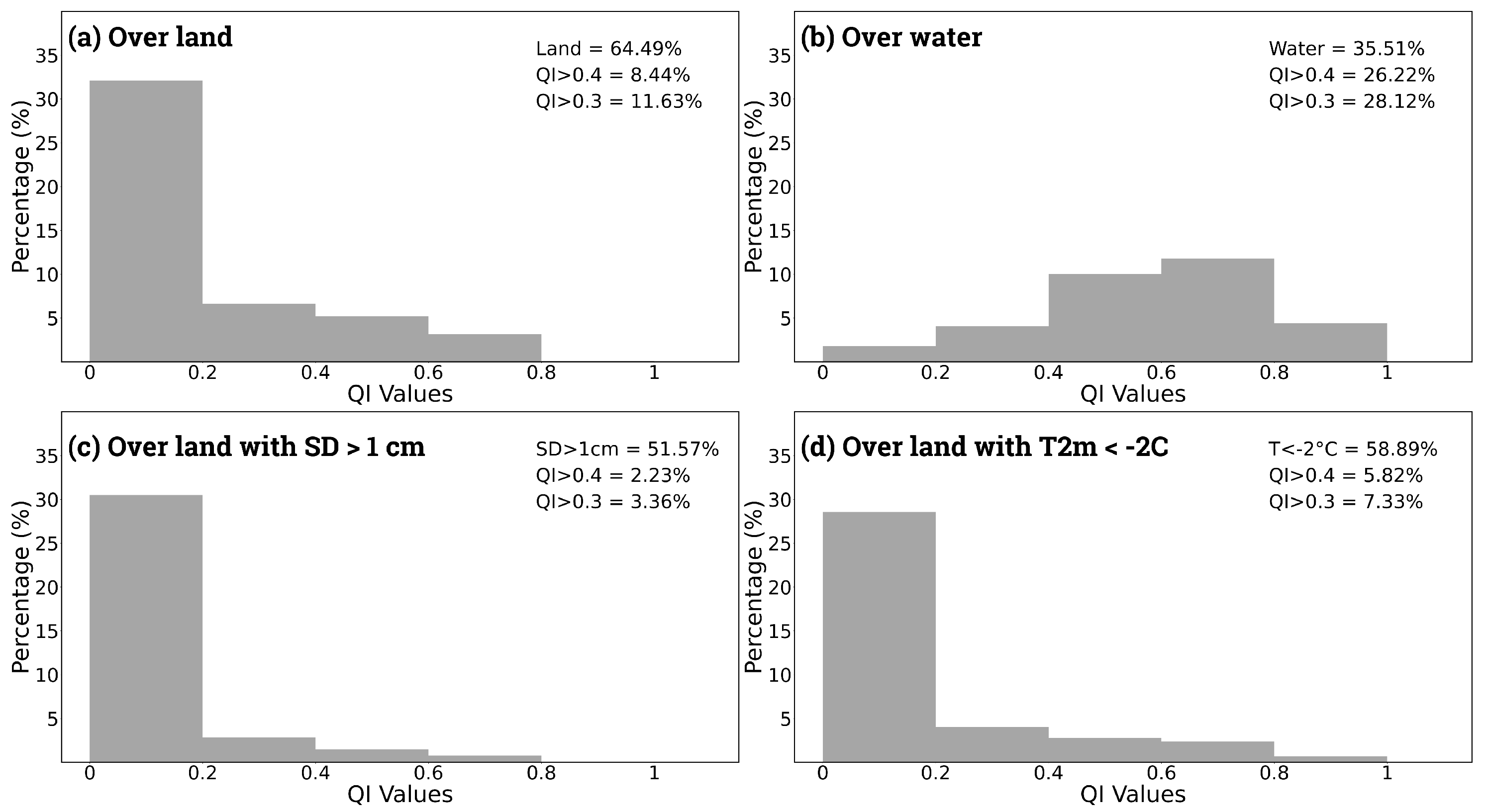
2.3. IMERG Quality Index

As explained in [58], correlation coefficients supplied by the Kalman smoother in CMORPH provide a measure of the relative skill for IMERG precipitation estimates [53]. The correlation coefficients for forward- and backward-propagated PMW estimates ($c_{fp}$ and $c_{bp}$) and for the IR estimate ($c_{ir}$) are combined after a variance-stabilizing transformation based on [59], as given in [58]’s Equation (5):

$$c_t=tanh\left(\sqrt{{arctanh}^2\left(c_{fp}\right)+{arctanh}^2\left(c_{bp}\right)+{arctanh}^2\left(c_{ir}\right)}\right)$$

(1)

The $c_t$ value actually corresponds to IMERG’s half-hourly quality index (QI).

Since the Early product is assimilated in CaPA in this study, with no backward propagation contribution to the IMERG estimates, only $c_{fp}$ and $c_{ir}$ are considered here. The IR contribution is included when the PMW propagation is greater than 90 min for the current half-hour precipitation estimate. Values of 0.4 and 0.6 for QI have been proposed to distinguish between a “red” class (from 0 to 0.4, dominated by the IR contribution with higher uncertainty), a “green” class (from 0.6 to 1.0, with more contribution from current PMW measurements and limited morphing), and a “yellow” class (from 0.4 to 0.6, an intermediate category with contribution from PMW but with more morphing) [35,58]. In this study, QI values of 0.3 and 0.4 are tested as thresholds in CaPA’s quality control, as explained in more detail below. The QI values from IMERG, provided every 30 min, are simply averaged over CaPA’s 6 h validity periods.

It should be mentioned that QI has negative values for land areas north of 60 degrees latitude, which covers a portion of the analysis domain shown in Figure 1. No IMERG information is considered or available over that region.

2.4. Objective Evaluation of CaPA Analyses

A leave-one-out cross-validation (LOOCV) approach is employed in this study to evaluate the quality of CaPA’s precipitation analyses. This technique is one of CaPA’s basic features and is actually part of the quality control process [16]. It is also a well-established component of ECCC’s official standards of verification for modifications and implementations related to CPA; see, for example, [17,42].

With LOOCV, CaPA’s two-dimensional statistical interpolation scheme is applied at the site of a subset of surface observations, assimilating all those in the vicinity but excluding the observation at that specific location. The LOOCV estimate is then compared with the actual observation at the site, which was excluded from assimilation, and the process is repeated in order to build error statistics. In the present study, these calculations are performed for all synoptic manual observations in the U.S. and Canada that pass CaPA’s quality control. An example of the spatial distribution of these manual observations is provided in Figure 1.

A set of categorical scores and metrics are computed with these error statistics and displayed as a function of selected precipitation thresholds. These metrics include the Frequency Bias Index (FBI), the Probability of Detection (POD), the False Alarm Ratio (FAR), and the Equitable Threat Score (ETS), as well as partial sums of total precipitation. Details for the calculation of these quantities are provided in Appendix A.

2.5. Snow Depth Analyses

Snow depth analyses from ECCC’s Canadian Land Data Assimilation System (CaLDAS) are used in this study to relate IMERG’s contribution in CaPA to the presence of snow on the ground. CaLDAS is a data assimilation system that provides land surface initial conditions for ECCC’s numerical weather and environmental prediction systems [60]. Analyses of soil moisture, surface temperature, and terrestrial snow are produced in real time by CaLDAS, every 3 h. The snow products from the CaLDAS implementation in ECCC’s 2.5 km National Surface and River Prediction System (NSRPS) are those compared in this study with the IMERG and CaPA precipitation fields. Details of this version of CaLDAS are provided in [61].

In CaLDAS-NSRPS, snow depth analyses are produced with a two-dimensional ensemble OI that combines information from an offline land surface first guess (or background) with the Snow and Interactive Multisensor Snow (IMS) 1 km daily snow product taken as observations. The ensemble contains 24 members. The land surface offline system is forced by CaPA’s precipitation analyses and by short-range numerical weather forecasts. The IMS product [62,63] is spatially aggregated to the 2.5 km national analysis grid, before bias removal and going through a thinning process (removing approximatively 50% of grid point observations). The ensemble mean of CaLDAS analyses is presented as the snow depth product for this study. It is linearly interpolated from 2.5 km to 10 km grid spacing in order to be directly comparable with the precipitation fields.

2.6. Screen-Level Air Temperature Dataset

Together with snow depth analyses, near-surface air temperature is also examined to inform on the nature of IMERG’s impact on CaPA’s wintertime precipitation analyses. The near-surface air temperature fields are extracted from short-range (7 h to 12 h) HRDPS forecasts. For diagnostics purposes, the 6-hourly temporal mean is estimated. In a manner similar to the snow analysis, the air temperature is linearly interpolated to this study’s 10 km analysis grid.

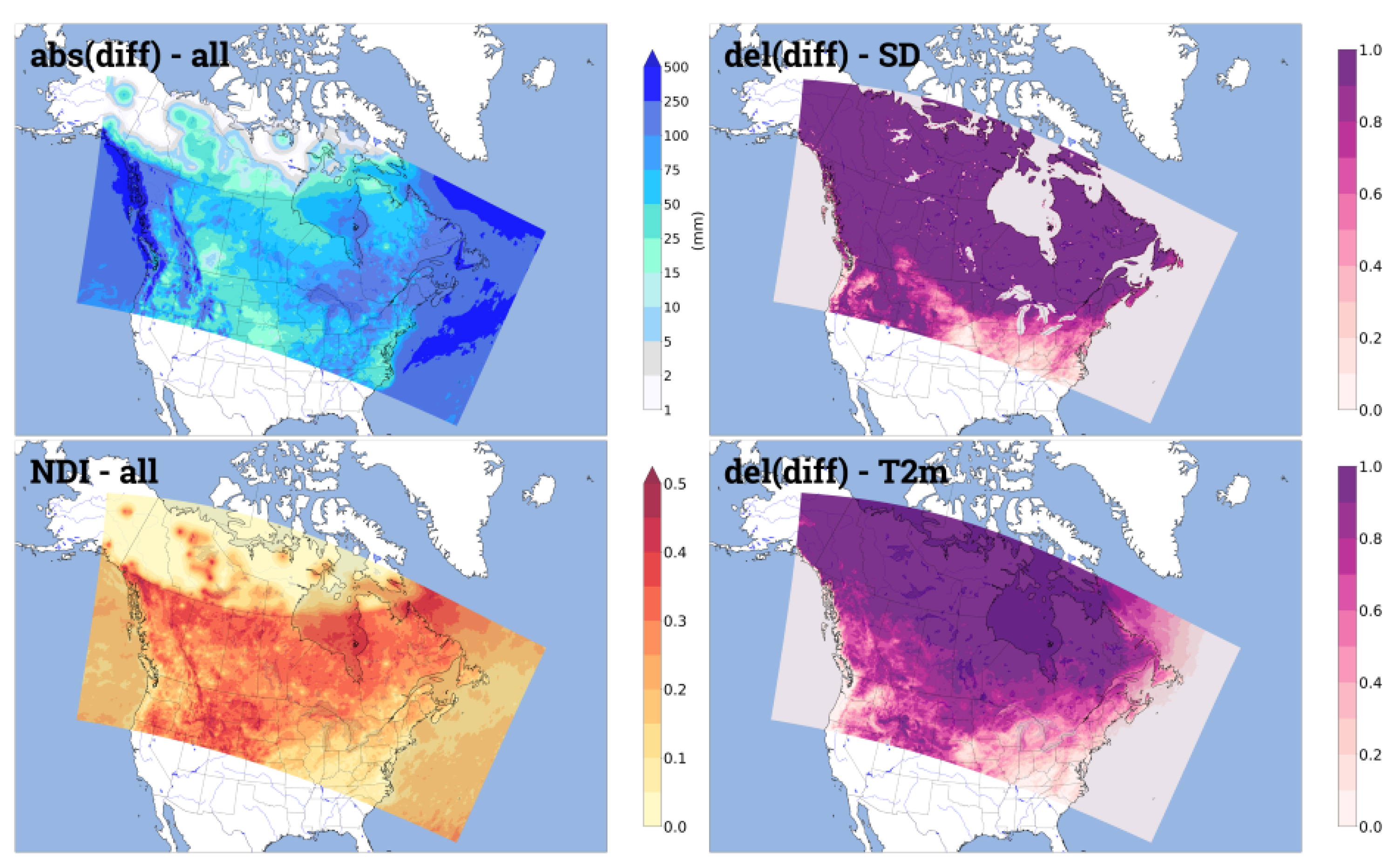
2.7. Diagnostics for IMERG Relative Contribution

The differences in CaPA’s precipitation analyses between the experiments with and without IMERG are used in this study to estimate the relative contribution of the satellite product. For each point on CaPA’s analysis grid, the sum of absolute precipitation differences is computed in this manner:

$$\sum |\Delta P_{IMERG}|=\sum _t^{winter}|P_{IMERG}-P_{CTRL}{|}_t$$

(2)

in which t is validity time for all CaPA’s analyses during the evaluation period, $P_{IMERG}$ is the 6-hourly precipitation analysis value for the CaPA IMERG experiments described in the next subsection, and $P_{CTRL}$ is the same but for the control experiment. The IMERG contribution is also presented with a normalized precipitation difference index, defined as follows:

$$NDI=\frac{\sum |\Delta P_{IMERG}|}{\sum P_{2x}}$$

(3)

where

$$\sum P_{2x}=\sum _t^{winter}{\left(P_{CTRL}+P_{IMERG}\right)}_t$$

(4)

These two diagnostics are also applied to estimate the IMERG contribution over snow-covered land surfaces and for areas where precipitation is assumed to be solid. In these cases,

$$\sum |\Delta P_{snow}|=\sum _t^{winter}|P_{IMERG}-P_{CTRL}{|}_t\mathcal{H}{(s_d-1.0)}_t$$

(5)

and

$$\sum |\Delta P_{solid}|=\sum _t^{winter}|P_{IMERG}-P_{CTRL}{|}_t\left(1.-\mathcal{H}{\left[T_{2m}-(-2.0)\right]}_t\right)$$

(6)

where $\mathcal{H}$ is the Heaviside function, $s_d$ is the mean snow depth (cm) during the 6-hourly analysis period, and $T_{2m}$ is the mean air temperature at the screen level (°C). In the figures and tables shown later, the IMERG contribution for these two situations are also normalized by the total absolute differences:

$$\begin{array}{ccc}\hfill Rel{\Delta }_{snow}=\frac{\sum |\Delta P_{snow}|}{\sum |\Delta P_{IMERG}|}& \hfill & \hfill Rel{\Delta }_{solid}=\frac{\sum |\Delta P_{solid}|}{\sum |\Delta P_{IMERG}|}\end{array}$$

(7)

The corresponding normalized indices are calculated as well:

$$\begin{array}{ccc}\hfill ND{I}_{snow}=\frac{\sum |\Delta P_{snow}|}{\sum P_{2x}}& \hfill & \hfill ND{I}_{solid}=\frac{\sum |\Delta P_{solid}|}{\sum P_{2x}}\end{array}$$

(8)

All the above diagnostics are either presented as maps, representative of the entire evaluation period, or in a table with values spatially averaged over all land surface points.

2.8. Experimental Setup

The numerical experiments are performed for the boreal winter season of 2021–2022. The assimilation cycles are initialized on 1 November 2021 and are run for five months, ending on 31 March 2022. To avoid ambiguity associated with spinup of CaPA’s error estimates from the variographic process, the first month is discarded and objective evaluation is performed for the last four months, from 1 December 2021 to 31 March 2022. For simplicity’s sake, this period is referred to as winter 2022 in this article. CaPA’s configuration is the same as ECCC’s RDPA system, with a 10 km grid spacing. Three experiments are performed and compared:

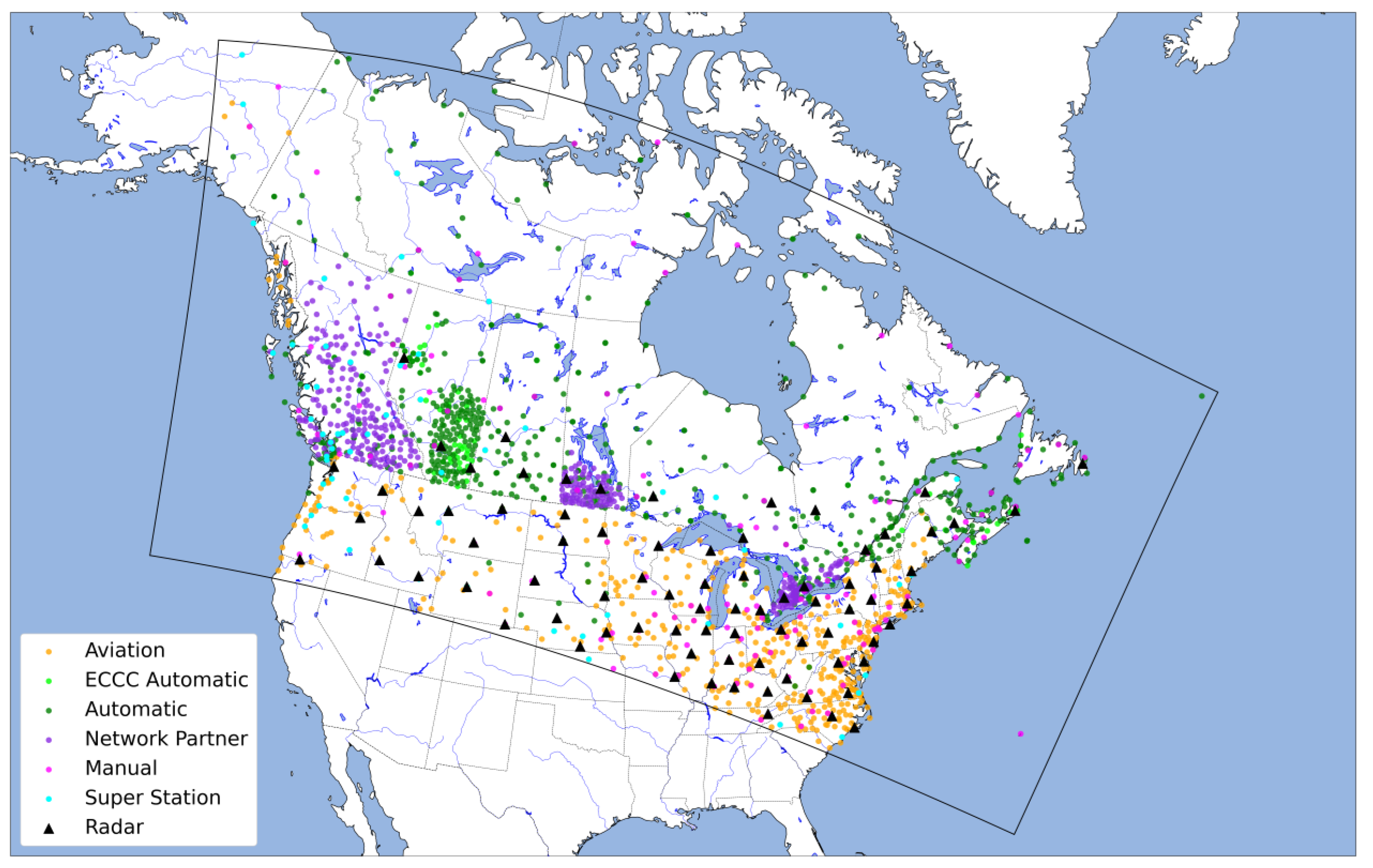
• CTRL is similar to what is used operationally at ECCC for the RDPA, except that no IMERG data are assimilated. To facilitate the interpretation of the results (i.e., to determine the impact of IMERG on the precipitation analyses), only observations from surface gauges and weather radars are assimilated.
• IMERG-ALL is the same configuration as CTRL, except that IMERG is assimilated with no quality control check, i.e., all available IMERG estimates are included in CaPA.
• IMERG-0p4 is the same configuration as CTRL, except that IMERG is only assimilated when the quality index (QI) is locally greater than a predetermined threshold, i.e., 0.4 for this experiment.
• IMERG-0p3 is the same as IMERG-0p4, except that a threshold of 0.3 is used instead of 0.4.

3. Results

The impact of including IMERG retrievals on CaPA’s precipitation wintertime analyses is first described in a qualitative manner with a case study. This description is provided for the CTRL and IMERG-ALL experiments and is followed by a more quantitative assessment based on CaPA’s objective evaluation with LOOCV, performed against synoptic manual observations available over the domain of interest and assimilated by CaPA (see Figure 1).

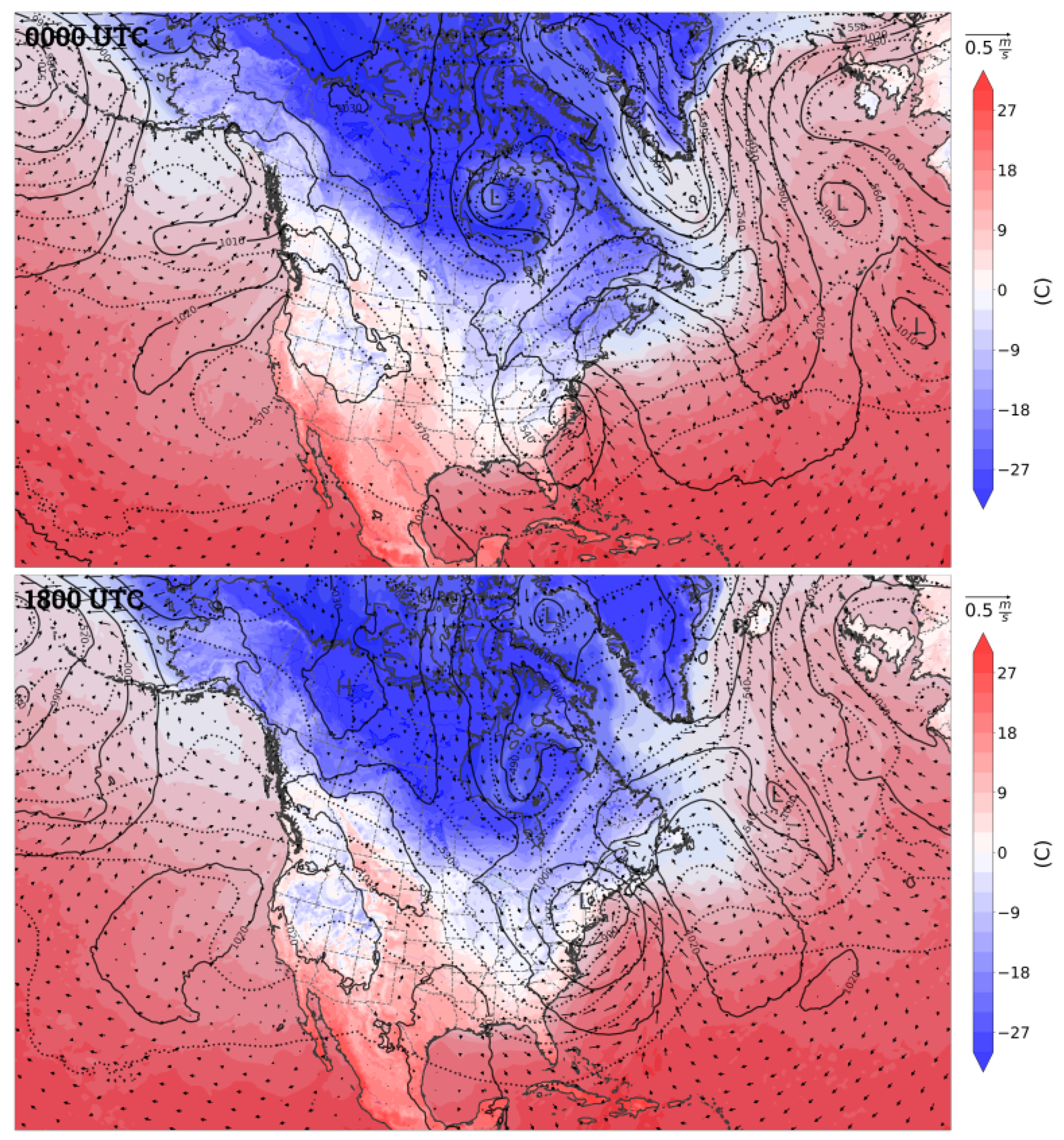
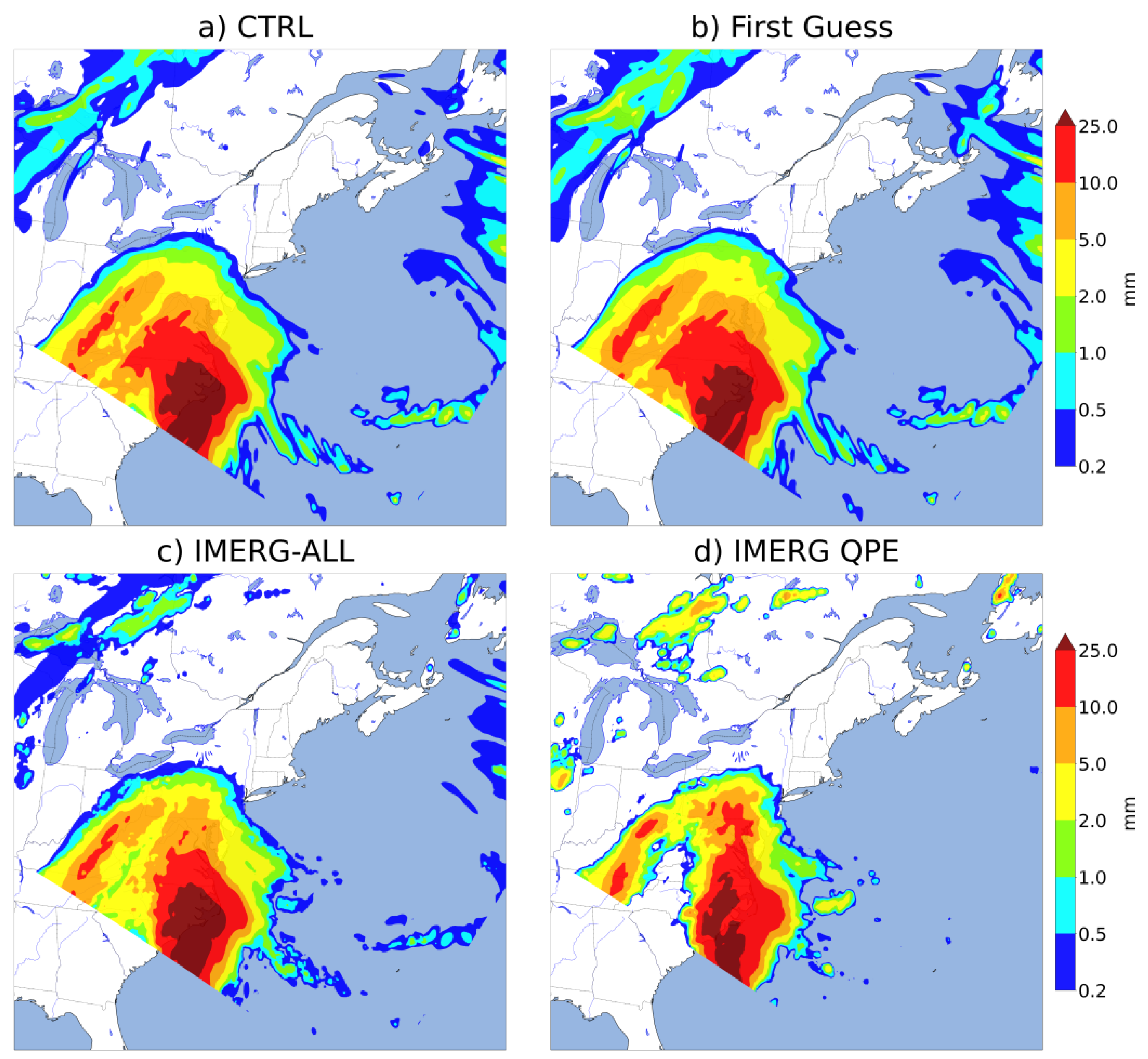
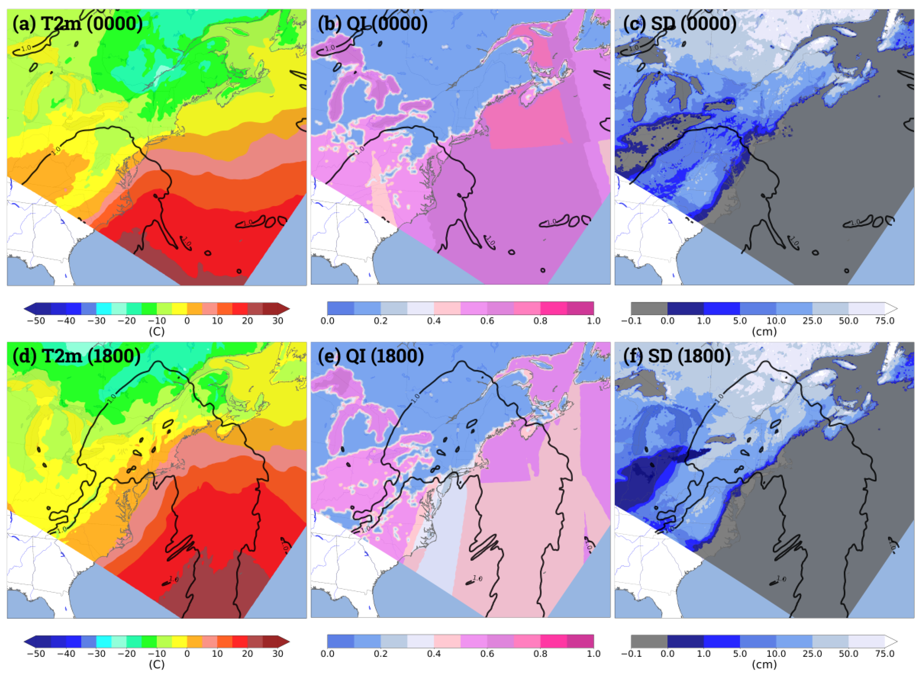
3.1. A Winter Case Study

On 17 January 2022, a large-scale meteorological system was responsible for substantial precipitation over the U.S. east coast and Canada’s eastern provinces. As presented in Figure 2, this important event is directly linked with the development and intensification of a surface low-pressure system moving northward from Virginia’s coast at 0000 UTC to New York state at 1800 UTC the same day. This development is supported by an upstream mid-tropospheric trough over the U.S. midwest at 0000 UTC, which becomes more in phase with surface features at 1800 UTC. The near-surface air temperature displays a sharp gradient near the low-pressure center, with warmer air (above 0 °C) over the ocean and colder air inland and northward. The temperature is near 0 °C along the coast in the vicinity of the low-pressure center.

The 6-hourly precipitation for that event is displayed in Figure 3 and Figure 4 for the hours preceding 0000 UTC and 1800 UTC on 17 January 2022. At 0000 UTC (Figure 3), the CaPA analysis for CTRL is close to the first guess (see panels a and b), indicating that the contribution from observations is small for that period. The analysis displays large precipitation amounts (greater than 25 mm) near the coast in association with warm frontal circulations. A narrower and less intense band is analyzed over land in colder air at the back of the meteorological system.

For that period, the spatial structures from the IMERG precipitation retrievals (referred to as “IMERG QPE” in the figure) are similar to the first guess and to CaPA’s CTRL analysis, but with sharper features (see Figure 3d). In particular, the gap zone between the two precipitation areas is more clearly defined for the IMERG product, with near-zero precipitation amounts. This is reflected in CaPA’s IMERG-ALL analysis, which exhibits slight differences with CTRL, especially in the area of that precipitation gap zone.

For the 6 h period preceding 1800 UTC on 17 January 2022, the precipitation structures have moved northward following the motion of the large-scale meteorological system. As can be seen in Figure 4, a long, wide, and intense precipitation band is analyzed by CaPA’s CTRL experiment over the Atlantic ocean in association with the system’s warm frontal zone (Figure 4a). Substantial precipitation is also found northwest of the low-pressure center, over southern Quebec and eastern Ontario. A narrow precipitation band extends to the southwest at the back of the system. Other smaller precipitation bands which appear to be caused by lake effects are also detected, just south of Lake Superior and east of Lake Michigan.

Again, the 6-hourly precipitation analysis from CTRL is very similar to the first guess (cf., Figure 4a,b). Over the Atlantic ocean, CTRL and the first guess are practically identical because no observations are assimilated over that area. For the IMERG retrievals (Figure 4d), the precipitation band over the ocean is more intense, smoother, and slightly wider than CTRL and the first guess. This has a direct impact on CaPA’s analysis in IMERG-ALL (panel c), whose structures have characteristics between CTRL and the IMERG retrievals.

The IMERG precipitation structures over land are on the other hand more disorganized and do not exhibit the spatial extension expected for that type of weather system. In fact, for that specific case, precipitation from IMERG is rather noisy and only covers a small area over land. This has a substantial impact on CaPA’s IMERG-ALL analysis over land, where CaPA’s analysis becomes more noisy and covers a smaller area. Also, the lake-effect bands near Lake Superior and Lake Michigan are less evident.

As expected, the precipitation analyses from the other two experiments, i.e., IMERG-0p4 and IMERG-0p3, are between what is shown in Figure 3 and Figure 4. These case studies are not presented here, but results from these other two experiments are examined in some details in the sections below, with emphasis on their objective evaluation and on the discussion concerning the role and impact of IMERG.

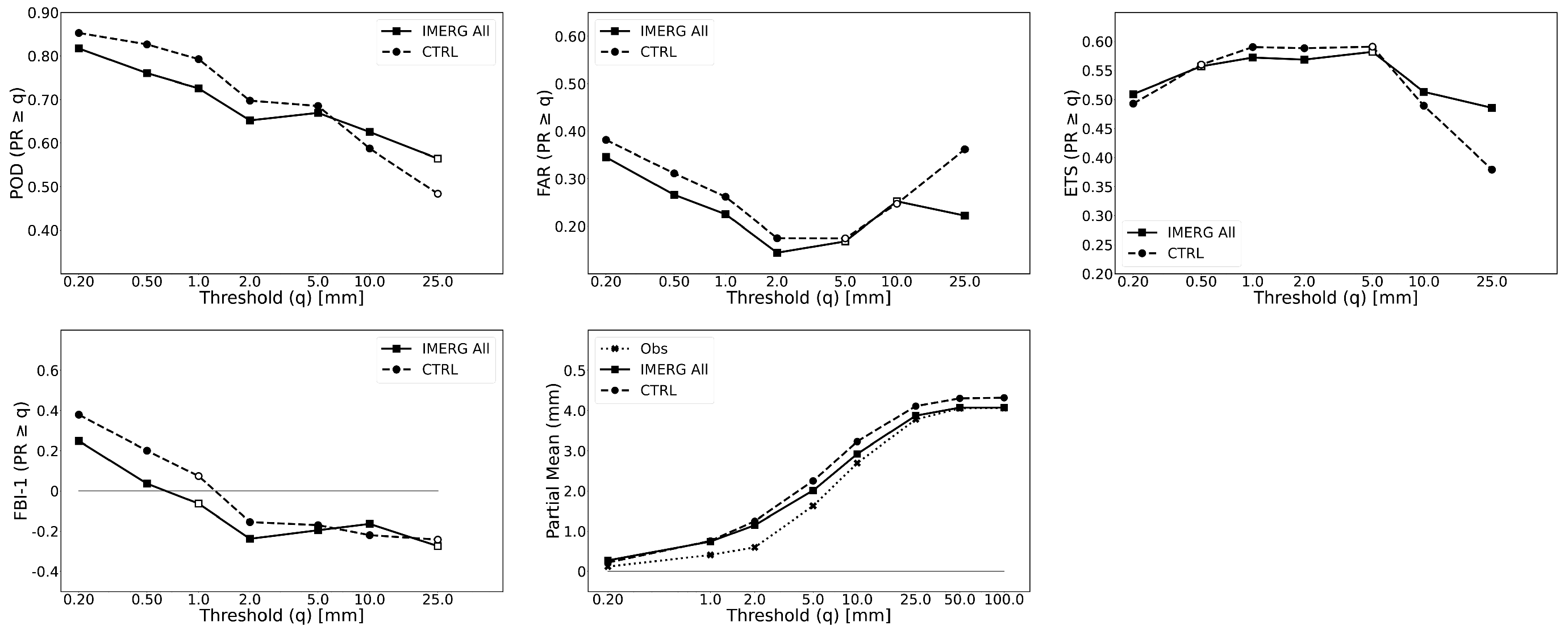
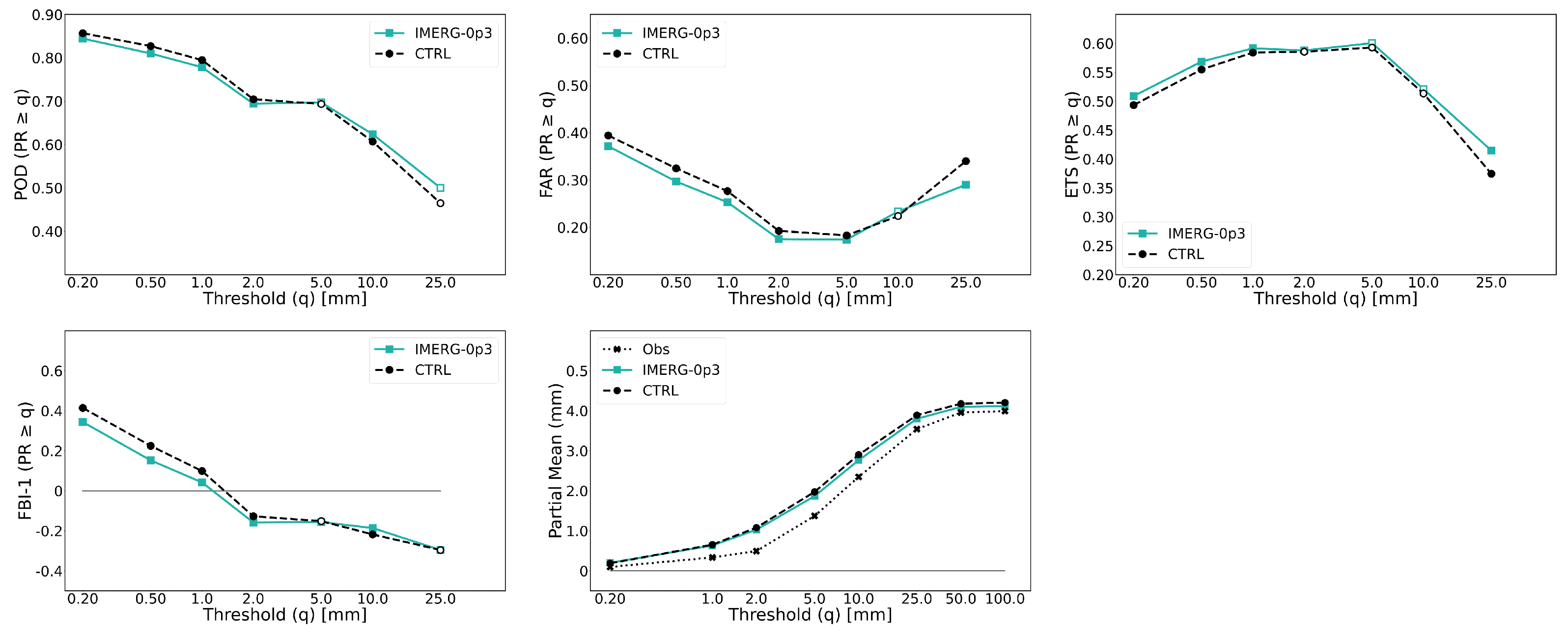
3.2. Objective Evaluation

Two IMERG experiments (IMERG-ALL and IMERG-0p4) are objectively evaluated against surface observations and compared with CTRL over the entire winter period, from 1 December 2021 to 31 March 2022, based on pairing with surface synoptic observations. A comparison between IMERG-ALL and CTRL is shown in Figure 5 and indicates that precipitation amounts are generally lowered when all IMERG retrievals are included in CaPA. The frequency bias is clearly decreased with IMERG-ALL, as shown in the lower left panel of Figure 5 for FBI-1. This is accompanied by a reduction in the partial means (lower right panel). For that season and over that region, assimilation of all IMERG retrievals has a beneficial impact for the precipitation amounts and for the frequency of precipitation events (at least for the smaller thresholds).

The effect on POD and FAR is consistent with the bias decrease. As expected, both detection (POD, upper left panel of Figure 5) and false alarms (FAR, upper middle panel) are lowered, meaning a worse performance concerning detection and better performance for false alarms. The overall impact on the accuracy of CaPA’s precipitation analyses, indicated here with ETS (upper right panel), is mostly negative. While ETS for the smallest precipitation threshold is improved, values for other thresholds (i.e., 1, 2, and 5 mm) are deteriorated. It should be mentioned that the differences found for the larger thresholds (i.e., 10 and 25 mm) should be examined with care due to the insufficient number of cases which does not allow for a robust statistical estimation of the quality difference between the two experiments.

Objective evaluation for the IMERG-0p4 experiment, in which IMERG is assimilated in CaPA only if its quality index has values greater than 0.4, is compared with CTRL in Figure 6. At first glance, the quality of CaPA’s analyses appears to be quite similar for the two experiments. The differences are in fact substantially smaller than what is depicted in Figure 5 for IMERG-ALL. Although slight, IMERG-0p4’s impact on CaPA’s analyses is in the same direction as IMERG-ALL concerning biases, detection, and false alarms, with a decrease for all these metrics. One distinction, however, is that the ETS score is improved for most thresholds with IMERG-0p4. But this improvement remains small, and overall, the results for both IMERG-ALL and IMERG-0p4 are in clear contrast with [20], which showed substantial improvement associated with the assimilation of IMERG in CaPA during the warm season.

4. Discussion

The results presented in the previous section inform on the potential effect of assimilating IMERG into CaPA during the cold season over Canada. Using the quality index to control which IMERG data are assimilated has a substantial impact on the objective evaluation of CaPA analyses. In this section, the sensitivity to the quality index is discussed, together with an estimation of the IMERG contribution to the precipitation analyses, with emphasis on spatial distribution, precipitation phase, and links to the presence of snow on the ground.

4.1. Choice and Optimization of QI Threshold

Several frequency distributions of QI are presented in Figure 7. The percentage values in that figure relate to the total number of analysis grid points over the entire domain, and do not sum to 100% for each individual panel. Also, grid points with negative QI values (over land north of 60 degrees latitude) are not included in the histograms, which only considers positive values of the quality index.

In Figure 7, the difference between land and water areas in terms of IMERG quality index is obvious. Over water, about 26.2% of points have a quality index greater than 0.4, while this number goes down to approximately 8.4% over land areas. This difference is even larger when considering relative occurrence (i.e., normalized by the percentage of land and water points). It goes from approximately 74% (i.e., 26.22/35.51) for water areas to about 13% (i.e., 8.44/64.49) over land. Looking at areas covered by snow over land, the percentage is as low as 2.2%. For land areas with air temperature below −2 °C, where precipitation is presumably in solid phase, the percentage of total points with a QI greater than 0.4 is approximately 5.8%.

When using a threshold of 0.4 for the quality index in IMERG-0p4, only a small fraction of the analysis grid is thus influenced (positively or negatively) by the assimilation of IMERG data. Considering the lack of impact noticed in Figure 6 for that QI threshold, it seems that a compromise is needed between that experiment and IMERG-ALL, in which all IMERG data are accepted in CaPA. In that context, an IMERG-0p3 experiment is performed in which the QI threshold is lowered to 0.3. As shown in Figure 7, this modification has the effect of increasing the percentages of assimilated points over land from 8.5% to 11.6%, from 2.2% to 3.4% over land areas covered by snow, and from 5.8% to 7.3% over land with cold temperatures (i.e., solid precipitation).

As expected and as can be seen in IMERG-0p3’s objective evaluation presented in Figure 8, the results for this new experiment mostly fall between the other two IMERG experiments, i.e., IMERG-ALL and IMERG-0p4. Biases (FBI and partial means), as well as POD and FAR, are all decreased compared with CTRL, but not as much as for IMERG-ALL (cf., Figure 5). A major distinction, however, is that the accuracy metric ETS is much improved (increased) with IMERG-0p3 for all precipitation thresholds. This suggests that the IMERG data added in CaPA’s assimilation process by decreasing the QI threshold positively contribute to the quality of CaPA’s analyses over the domain of interest for that specific winter season.

4.2. Quality Index and IMERG Contribution for Case Study

The role of QI can also be examined in the context of the 17 January 2022 case study presented in Section 3.1 with Figure 3 and Figure 4. For that case, the IMERG’s contribution to CaPA’s 6-hourly precipitation analysis is small but positive at 0000 UTC on 17 January 2022 (Figure 3). The impact is greater at 1800 UTC, but appears to corrupt precipitation structures over land at that time (Figure 4).

This IMERG contribution is better understood when looking at QI maps in Figure 9, presented with near-surface air temperature and snow depth on the ground. The upper panels of that figure, valid at 0000 UTC on 17 January 2022, indicate that the QI is relatively large (i.e., QI > 0.4) for areas just south of the Great Lakes where most of the precipitation is located. At that time, air temperature is near 0 °C for most of that area, with snow depth on the order of 5 cm according to CaLDAS. Large QI values are why the inclusion of IMERG leads to improved CaPA analysis at that time, in spite of the shallow snow pack coverage.

The situation is different at 1800 UTC on 17 January 2022 when the QI is slightly decreased over southern areas where precipitation occurred earlier (see lower panels of Figure 9). Based on air temperature and snow depth maps shown in the same figure, precipitation over that southern region is most likely in solid phase. Importantly, most precipitation at 1800 UTC occurs over areas to the north (southern Quebec and Ontario, Canada’s maritime provinces, and northeastern U.S. states) where the QI has values less than 0.2. The air temperature is clearly below 0 °C over these areas, with a deeper snowpack (25 cm and more). This could explain why IMERG has a detrimental impact over land for the CaPA analysis valid at that time (see Figure 4). Although not shown here, results from the IMERG-0p4 and IMERG-0p3 experiments, in which IMERG data are still assimilated at 0000 UTC over land, but are rejected (not used) at 1800 UTC, lead to a better compromise between the first guess and IMERG product for that case study.

4.3. IMERG Contribution over Land, Snow, and Cold Areas

The quality of CaPA’s 6-hourly precipitation analyses appears to be improved when assimilating IMERG data, but only when these data are carefully selected based on the IMERG quality index (see Figure 8). How much and where does IMERG modify CaPA’s precipitation analyses, and does it have an impact over areas covered by snow or for snowfall precipitation (approximated in this study by areas where air temperature is below −2 °C)? Are the gains associated with IMERG only due to its good performance for rainfall events?

In an attempt to answer these questions, Figure 10 presents maps showing some of the metrics defined in Section 2.7 to quantify IMERG’s contribution by comparing CaPA’s precipitation analyses with and without IMERG. The upper-left panel in Figure 10 reveals that the sum of the absolute differences between IMERG-ALL and CTRL can be relatively large in some regions. As expected, the greatest increments are found over oceans. But IMERG’s impact is also substantial over land areas, i.e., over western Canada, eastern U.S. and Canada, and central Canada. Total precipitation amounts, summed in absolute values over the entire winter 2022 season, are greater than 50 mm over large land portions of the domain, and even above 100 mm for some areas (e.g., near the border between Quebec and Ontario, and in British Columbia). It should be noted that IMERG also contributes to CaPA’s analyses north of 60 degrees latitude, in Canada’s Northwest Territories, and in Alaska, in association with the presence of several lakes (some of them very large). Similarly, the differences are also considerable over the Great Lakes area.

When considered relative to CaPA’s CTRL seasonal precipitation amounts, using the NDI index defined in Equation (3), IMERG’s impact appears to be complementary to its contribution in absolute values. As shown in the lower-left panel of Figure 10, NDI between IMERG-ALL and CTRL is larger over Canada’s northern areas (just below 60 degrees latitude) and over northwestern U.S. states. The NDI is also substantial over central Canada. Even if IMERG’s contribution is smaller in absolute values over these areas, its relative contribution is actually larger.

The right panels in Figure 10 indicate that for that winter season, most of the differences between IMERG-ALL and CTRL over land in Canada occur in areas covered by snow and with air temperatures below −2 °C. Considering the entire domain, only areas in the southeastern portion of the domain (in the U.S.) have most of the differences over land not covered by snow. The partitioning of IMERG’s contribution between snowfall and rainfall is more balanced, with a larger land portion of the domain with relative differences below 0.5 (50%). These areas are mostly in the northeastern U.S., southeastern Canada, and in states and provinces near the Pacific west coast. This indicates that the impact found in CaPA’s evaluation metrics for IMERG-ALL, as shown in Figure 5, mostly occurs over snow-covered land surfaces, but not necessarily as snowfall accumulations since the ratio between rainfall and snowfall seems more balanced.

When using the quality index (QI) to control the assimilation of IMERG in CaPA, the absolute differences and NDI compared with CTRL are substantially smaller, as can be seen in Figure 11. By construction, both the absolute differences (left panels) and NDI (right panels) are larger for IMERG-0p3 compared to those for IMERG-0p4. For both experiments, the IMERG contribution is mostly over the U.S. portion of the domain, and over water bodies. In Canada, IMERG has some impact on CaPA’s analyses over British Columbia, southern Quebec, southern Ontario, and in the Northwestern Territories, as well as Nunavut. In the right panels of that same figure, the NDI is found to be small over most continental areas, except for those dominated by the presence of lakes, and for north central U.S. states. For most of Canada, the NDI is below 0.1. These results suggest that the positive impact demonstrated with IMERG-0p3 (Figure 8) is most likely related to IMERG’s influence in the southern portion of the domain, where a combination of rainfall and snowfall occurs.

Spatial means (over the land portion of the analysis domain shown in Figure 1) of temporal means of NDI and sums of absolute differences (for the entire winter 2022 season) are presented in

Table 1. IMERG’s contribution to CaPA’s precipitation analyses over land.

	$\mathit{NDI}$	${\mathit{NDI}}_{\mathit{snow}}$	${\mathit{NDI}}_{\mathit{solid}}$	$\sum |\Delta {\mathit{P}}_{\mathit{IMERG}}|$	$\sum |\Delta {\mathit{P}}_{\mathit{snow}}|$	$\sum |\Delta {\mathit{P}}_{\mathit{solid}}|$
				(mm)	(mm)	(mm)
IMERG-ALL	0.21	0.18	0.16	73.0	58.3	44.2
IMERG-0p4	0.02	0.02	0.02	11.7	7.4	5.3
IMERG-0p3	0.05	0.04	0.03	22.2	14.1	10.0

. These numbers are consistent with the interpretation above for Figure 10 and Figure 11. They confirm the relatively large IMERG contribution in the IMERG-ALL experiment, which is mostly found over snow-covered surfaces and to a lesser extent in areas with air temperatures below −2 °C. The numbers also show the drastic diminution of IMERG’s role over land with IMERG-0p4, and the slight increase when the QI threshold is lowered to 0.3 (i.e., in IMERG-0p3, compared with IMERG-0p4). Interestingly, data for IMERG-0p3 reveal that more than half of the absolute differences occur over snow-covered surfaces (i.e., 14.1 mm compared with 22.2 mm in total). This contribution is less in cold areas where precipitation is assumed to be snowfall (i.e., 10.0 mm compared with 22.2 mm).

5. Summary and Conclusions

The impact of including IMERG in CaPA for wintertime precipitation analyses is investigated in this study. In the context of CaPA’s 10 km deterministic version, the results indicate that IMERG can indeed improve wintertime precipitation analyses, but only if adequate quality control is performed. Based on a case study and on a set of objective evaluation metrics, including IMERG in CaPA leads to less precipitation during the winter 2022 season (generally an improvement for that specific year) and to either improvement or deterioration of ETS, depending on the level of quality control applied to IMERG data prior to assimilation.

With a QI threshold of 0.3, IMERG is found to improve ETS in a meaningful manner compared with the control experiment in which no IMERG data are assimilated. Insights based on spatial and temporal diagnostics reveal that IMERG’s contribution to that successful experiment (IMERG-0p3) mostly occurs in the southern parts of the domain, where a greater fraction of precipitation is more likely to fall as rain. These diagnostics, when averaged over the entire domain, indicate that CaPA’s analyses are also modified by IMERG in a substantial manner in areas covered by snow (about 50% of the absolute differences) and where air temperature is below −2 °C (where precipitation is assumed to be in solid phase, about 45%).

These conclusions are based on a single winter season and might change if more years are considered as part of the objective evaluation. Also, the evaluation was performed for the total precipitation without distinction of phases. It would certainly be of interest to determine IMERG’s impact on the liquid and solid components of CaPA’s precipitation analyses. But CaPA does not produce distinct analyses for each phase; it rather generates analyses for total precipitation. In Canada, information on precipitation phase is not available from the surface observational networks assimilated in CaPA. Moreover, objective evaluation for solid precipitation is more uncertain due to large errors associated with surface measurements, especially in meteorological situations with moderate-to-strong surface winds.

Several related studies are expected following this present effort:

• The evaluation could be performed over several years, in preparation for a possible implementation in ECCC’s operational systems;
• It would be interesting to determine if the new version of IMERG, V07 [64], performs better than V06 when assimilated in CaPA;
• The role and impact of IMERG should be examined in other configurations of CaPA, in particular the high-resolution deterministic and ensemble versions producing analyses at 2.5 km grid spacing;
• A more exhaustive series of tests should be conducted to determine the optimal value of the QI threshold for its assimilation in CaPA; with the use of IMERG V07, it is possible that lower threshold values could be used for the QI;
• Alternatively, CaPA’s analysis error could be estimated for various QIs to automatically determine optimal threshold values, varying with seasons.

The results obtained in this study are likely to be combined with other recent changes to the precipitation analysis system, all demonstrating a positive impact on CaPA’s wintertime products.

References

1. Verdin, A.; Rajagopalan, B.; Kleiber, W.; Funk, C. A Bayesian kriging approach for blending satellite and ground precipitation observations. Water Resour. Res. 2015, 51, 908–921. [Google Scholar] [CrossRef]
2. Contractor, S.; Donat, M.G.; Alexander, L.V.; Ziese, M.; Meyer-Christoffer, A.; Schneider, U.; Rustemeier, E.; Becker, A.; Durre, I.; Vose, R.S. Rainfall Estimates on a Gridded Network (REGEN)–a global land-based gridded dataset of daily precipitation from 1950 to 2016. Hydrol. Earth Syst. Sci. 2020, 24, 919–943. [Google Scholar] [CrossRef]
3. Joyce, R.J.; Janowiak, J.E.; Arkin, P.A.; Xie, P. CMORPH: A method that produces global precipitation estimates from passive microwave and infrared data at high spatial and temporal resolution. J. Hydrometeorol. 2004, 5, 487–503. [Google Scholar] [CrossRef]
4. Ashouri, H.; Lin Hsu, K.; Sorooshian, S.; Braithwaite, D.; Knapp, K.; Cecil, D.; Nelson, B.; Prat, O. PERSIANN-CDR: Daily precipitation climate data record from multisatellite observations for hydrological and climate studies. Bull. Am. Meteorol. Soc. 2015, 96, 69–84. [Google Scholar] [CrossRef]
5. Sadeghi, M.; Nguyen, P.; Hsu, K.; Sorooshian, S. Improving near real-time precipitation estimation using a U-Net convolutional neural network and geographical information. Environ. Model. Softw. 2020, 134, 104856. [Google Scholar] [CrossRef]
6. Wang, C.; Xu, J.; Tang, G.; Yang, Y.; Hong, Y. Infrared precipitation estimation using convolutional neural network. IEEE Trans. Geosci. Remote Sens. 2020, 58, 8612–8625. [Google Scholar] [CrossRef]
7. Hersbach, H.; Bell, B.; Berrisford, P.; Hirahara, S.; Horányi, A.; Muñoz-Sabater, J.; Nicolas, J.; Peubey, C.; Radu, R.; Schepers, D.; et al. The ERA5 global reanalysis. Q. J. R. Meteorol. Soc. 2020, 146, 1999–2049. [Google Scholar] [CrossRef]
8. Gasset, N.; Fortin, V.; Dimitrijevic, M.; Carrera, M.; Bilodeau, B.; Muncaster, R.; Gaborit, É.; Roy, G.; Pentcheva, N.; Bulat, M.; et al. A 10 km North American precipitation and land-surface reanalysis based on the GEM atmospheric model. Hydrol. Earth Syst. Sci. 2021, 25, 4917–4945. [Google Scholar] [CrossRef]
9. Tapiador, F.J.; Turk, F.J.; Petersen, W.; Hou, A.Y.; García-Ortega, E.; Machado, L.A.; Angelis, C.F.; Salio, P.; Kidd, C.; Huffman, G.J.; et al. Global precipitation measurement: Methods, datasets and applications. Atmos. Res. 2012, 104, 70–97. [Google Scholar] [CrossRef]
10. Tapiador, F.; Navarro, A.; Levizzani, V.; García-Ortega, E.; Huffman, G.; Kidd, C.; Kucera, P.; Kummerow, C.; Masunaga, H.; Petersen, W.; et al. Global precipitation measurements for validating climate models. Atmos. Res. 2017, 197, 1–20. [Google Scholar] [CrossRef]
11. Sun, Q.; Miao, C.; Duan, Q.; Ashouri, H.; Sorooshian, S.; Hsu, K.L. A review of global precipitation data sets: Data sources, estimation, and intercomparisons. Rev. Geophys. 2018, 56, 79–107. [Google Scholar] [CrossRef]
12. Sharifi, E.; Brocca, L. Monitoring precipitation from space: Progress, challenges, and opportunities. Precip. Sci. 2022, 239–255. [Google Scholar]
13. Satgé, F.; Defrance, D.; Sultan, B.; Bonnet, M.P.; Seyler, F.; Rouché, N.; Pierron, F.; Paturel, J.E. Evaluation of 23 gridded precipitation datasets across West Africa. J. Hydrol. 2020, 581, 124412. [Google Scholar] [CrossRef]
14. Prakash, S. Performance assessment of CHIRPS, MSWEP, SM2RAIN-CCI, and TMPA precipitation products across India. J. Hydrol. 2019, 571, 50–59. [Google Scholar] [CrossRef]
15. Zhang, J.; Howard, K.; Langston, C.; Kaney, B.; Qi, Y.; Tang, L.; Grams, H.; Wang, Y.; Cocks, S.; Martinaitis, S.; et al. Multi-Radar Multi-Sensor (MRMS) quantitative precipitation estimation: Initial operating capabilities. Bull. Am. Meteorol. Soc. 2016, 97, 621–638. [Google Scholar] [CrossRef]
16. Lespinas, F.; Fortin, V.; Roy, G.; Rasmussen, P.; Stadnyk, T. Performance evaluation of the Canadian Precipitation Analysis (CaPA). J. Hydrometeorol. 2015, 16, 2045–2064. [Google Scholar] [CrossRef]
17. Fortin, V.; Roy, G.; Donaldson, N.; Mahidjiba, A. Assimilation of radar quantitative precipitation estimations in the Canadian Precipitation Analysis (CaPA). J. Hydrol. 2015, 531, 296–307. [Google Scholar] [CrossRef]
18. Fortin, V.; Roy, G.; Stadnyk, T.; Koenig, K.; Gasset, N.; Mahidjiba, A. Ten years of science based on the Canadian Precipitation Analysis: A CaPA system overview and literature review. Atmosphere-Ocean 2018, 56, 178–196. [Google Scholar] [CrossRef]
19. Goodison, B.E.; Louie, P.Y.; Yang, D. WMO Solid Precipitation Measurement Intercomparison. Technical Report WMO/TD-No. 872, World Meteorological Organization, Geneva, Switzerland. 1998. Available online: https://library.wmo.int/records/item/28336-wmo-solid-precipitation-measurement-intercomparison (accessed on 20 June 2024).
20. Lespinas, F.; Roy, G.; Mahidjiba, A.; Fortin, V. Regional Deterministic Precipitation Analysis System (CaPA-RDPA). Technical Report, Environment and Climate Change Canada. 2021. Available online: https://collaboration.cmc.ec.gc.ca/cmc/cmoi/product_guide/docs/lib/technote_capa_rdpa-500_e.pdf (accessed on 20 June 2024).
21. Boluwade, A.; Stadnyk, T.; Fortin, V.; Roy, G. Assimilation of precipitation estimates from the integrated multisatellite retrievals for GPM (IMERG, early run) in the Canadian Precipitation Analysis (CaPA). J. Hydrol. Reg. Stud. 2017, 14, 10–22. [Google Scholar] [CrossRef]
22. Huffman, G.; Bolvin, D.; Braithwaite, D.; Hsu, K.; Joyce, R.; Kidd, C.; Nelkin, E.; Sorooshian, S.; Tan, J.; Xie, P. Algorithm Theoretical Basis Document (ATBD) Version 06 NASA Global Precipitation Measurement (GPM) Integrated Multi-Satellite Retrievals for GPM (IMERG). Technical Report, National Aeronautics and Space Administration, Washington, DC, USA. 2019. Available online: https://gpm.nasa.gov/sites/default/files/2020-05/IMERG_ATBD_V06.3.pdf (accessed on 20 June 2024).
23. Huffman, G.J.; Bolvin, D.T.; Braithwaite, D.; Hsu, K.L.; Joyce, R.J.; Kidd, C.; Nelkin, E.J.; Sorooshian, S.; Stocker, E.F.; Tan, J.; et al. Integrated multi-satellite retrievals for the Global Precipitation Measurement (GPM) mission (IMERG). Satell. Precip. Meas. 2020, 1, 343–353. [Google Scholar]
24. Hou, A.Y.; Kakar, R.K.; Neeck, S.; Azarbarzin, A.A.; Kummerow, C.D.; Kojima, M.; Oki, R.; Nakamura, K.; Iguchi, T. The Global Precipitation Measurement mission. Bull. Am. Meteorol. Soc. 2014, 95, 701–722. [Google Scholar] [CrossRef]
25. Tan, J.; Huffman, G.J.; Bolvin, D.T.; Nelkin, E.J. IMERG V06: Changes to the morphing algorithm. J. Atmos. Ocean. Technol. 2019, 36, 2471–2482. [Google Scholar] [CrossRef]
26. Pradhan, R.K.; Markonis, Y.; Godoy, M.R.V.; Villalba-Pradas, A.; Andreadis, K.M.; Nikolopoulos, E.I.; Papalexiou, S.M.; Rahim, A.; Tapiador, F.J.; Hanel, M. Review of GPM IMERG performance: A global perspective. Remote Sens. Environ. 2022, 268, 112754. [Google Scholar] [CrossRef]
27. Dezfuli, A.K.; Ichoku, C.M.; Huffman, G.J.; Mohr, K.I.; Selker, J.S.; Van De Giesen, N.; Hochreutener, R.; Annor, F.O. Validation of IMERG precipitation in Africa. J. Hydrometeorol. 2017, 18, 2817–2825. [Google Scholar] [CrossRef] [PubMed]
28. Foelsche, U.; Kirchengast, G.; Fuchsberger, J.; Tan, J.; Petersen, W.A. Evaluation of GPM IMERG Early, Late, and Final rainfall estimates using WegenerNet gauge data in southeastern Austria. Hydrol. Earth Syst. Sci. 2017, 21, 6559–6572. [Google Scholar]
29. Mohammed, S.A.; Hamouda, M.A.; Mahmoud, M.T.; Mohamed, M.M. Performance of GPM-IMERG precipitation products under diverse topographical features and multiple-intensity rainfall in an arid region. Hydrol. Earth Syst. Sci. Discuss. 2020, 1–27. [Google Scholar]
30. Tang, G.; Clark, M.P.; Papalexiou, S.M.; Ma, Z.; Hong, Y. Have satellite precipitation products improved over last two decades? A comprehensive comparison of GPM IMERG with nine satellite and reanalysis datasets. Remote Sens. Environ. 2020, 240, 111697. [Google Scholar] [CrossRef]
31. Reichle, R.H.; Liu, Q.; Ardizzone, J.V.; Crow, W.T.; De Lannoy, G.J.; Kimball, J.S.; Koster, R.D. IMERG precipitation improves the SMAP Level-4 soil moisture product. J. Hydrometeorol. 2023, 24, 1699–1723. [Google Scholar] [CrossRef]
32. Moazami, S.; Najafi, M. A comprehensive evaluation of GPM-IMERG V06 and MRMS with hourly ground-based precipitation observations across Canada. J. Hydrol. 2021, 594, 125929. [Google Scholar] [CrossRef]
33. Song, Y.; Broxton, P.D.; Ehsani, M.R.; Behrangi, A. Assessment of snowfall accumulation from satellite and reanalysis products using SNOTEL observations in Alaska. Remote Sens. 2021, 13, 2922. [Google Scholar] [CrossRef]
34. Eckert, E.; Hudak, D.; Mekis, É.; Rodriguez, P.; Zhao, B.; Mariani, Z.; Melo, S.; Strong, K.; Walker, K.A. Validation of the final monthly integrated multisatellite retrievals for GPM (IMERG) Version 05 and Version 06 with ground-based precipitation gauge measurements across the Canadian Arctic. J. Hydrometeorol. 2022, 23, 715–731. [Google Scholar] [CrossRef]
35. Zhao, B.; Hudak, D.; Rodriguez, P.; Mekis, E.; Brunet, D.; Eckert, E.; Melo, S. Assessment of IMERG V06 satellite precipitation products in the Canadian Great Lakes region. J. Hydrometeorol. 2023, 24, 1017–1037. [Google Scholar] [CrossRef]
36. Chen, H.; Yong, B.; Gourley, J.J.; Liu, J.; Ren, L.; Wang, W.; Hong, Y.; Zhang, J. Impact of the crucial geographic and climatic factors on the input source errors of GPM-based global satellite precipitation estimates. J. Hydrol. 2019, 575, 1–16. [Google Scholar] [CrossRef]
37. Arabzadeh, A.; Behrangi, A. Investigating various products of IMERG for precipitation retrieval over surfaces with and without snow and ice cover. Remote Sens. 2021, 13, 2726. [Google Scholar] [CrossRef]
38. Munchak, S.J.; Skofronick-Jackson, G. Evaluation of precipitation detection over various surfaces from passive microwave imagers and sounders. Atmos. Res. 2013, 131, 81–94. [Google Scholar] [CrossRef]
39. Liu, G.; Seo, E.K. Detecting snowfall over land by satellite high-frequency microwave observations: The lack of scattering signature and a statistical approach. J. Geophys. Res. Atmos. 2013, 118, 1376–1387. [Google Scholar] [CrossRef]
40. Skofronick-Jackson, G.M.; Johnson, B.T.; Munchak, S.J. Detection thresholds of falling snow from satellite-borne active and passive sensors. IEEE Trans. Geosci. Remote Sens. 2013, 51, 4177–4189. [Google Scholar] [CrossRef]
41. Mahfouf, J.F.; Brasnett, B.; Gagnon, S. A Canadian Precipitation Analysis (CaPA) project: Description and preliminary results. Atmosphere-Ocean 2007, 45, 1–17. [Google Scholar] [CrossRef]
42. Khedhaouiria, D.; Bélair, S.; Fortin, V.; Roy, G.; Lespinas, F. High-resolution (2.5 km) ensemble precipitation analysis across Canada. J. Hydrometeorol. 2020, 21, 2023–2039. [Google Scholar] [CrossRef]
43. Côté, J.; Gravel, S.; Méthot, A.; Patoine, A.; Roch, M.; Staniforth, A. The operational CMC–MRB global environmental multiscale (GEM) model. Part I: Design considerations and formulation. Mon. Weather Rev. 1998, 126, 1373–1395. [Google Scholar] [CrossRef]
44. Côté, J.; Desmarais, J.G.; Gravel, S.; Méthot, A.; Patoine, A.; Roch, M.; Staniforth, A. The operational CMC–MRB global environmental multiscale (GEM) model. Part II: Results. Mon. Weather Rev. 1998, 126, 1397–1418. [Google Scholar] [CrossRef]
45. Girard, C.; Plante, A.; Desgagné, M.; McTaggart-Cowan, R.; Côté, J.; Charron, M.; Gravel, S.; Lee, V.; Patoine, A.; Qaddouri, A.; et al. Staggered vertical discretization of the Canadian Environmental Multiscale (GEM) model using a coordinate of the log-hydrostatic-pressure type. Mon. Weather Rev. 2014, 142, 1183–1196. [Google Scholar] [CrossRef]
46. Husain, S.Z.; Girard, C. Impact of consistent semi-Lagrangian trajectory calculations on numerical weather prediction performance. Mon. Weather Rev. 2017, 145, 4127–4150. [Google Scholar] [CrossRef]
47. Creutin, J.; Delrieu, G.; Lebel, T. Rain measurement by raingage-radar combination: A geostatistical approach. J. Atmos. Ocean. Technol. 1988, 5, 102–115. [Google Scholar] [CrossRef]
48. Chiles, J.P.; Delfiner, P. Geostatistics: Modeling Spatial Uncertainty; John Wiley & Sons: Hoboken, NJ, USA, 2012; Volume 713. [Google Scholar]
49. Roy, G.; Mahidjiba, A. High Resolution Deterministic Precipitation Analysis System (CaPA-HRDPA). Technical Report, Environment and Climate Change Canada. 2018. Available online: https://collaboration.cmc.ec.gc.ca/cmc/cmoi/product_guide/docs/lib/technote_capa_hrdpa-450_e.pdf (accessed on 20 June 2024).
50. Kummerow, C.; Hong, Y.; Olson, W.; Yang, S.; Adler, R.; McCollum, J.; Ferraro, R.; Petty, G.; Shin, D.B.; Wilheit, T. The evolution of the Goddard Profiling Algorithm (GPROF) for rainfall estimation from passive microwave sensors. J. Appl. Meteorol. 2001, 40, 1801–1820. [Google Scholar] [CrossRef]
51. Kummerow, C.D.; Ringerud, S.; Crook, J.; Randel, D.; Berg, W. An observationally generated a priori database for microwave rainfall retrievals. J. Atmos. Ocean. Technol. 2011, 28, 113–130. [Google Scholar] [CrossRef]
52. Kummerow, C.D.; Randel, D.L.; Kulie, M.; Wang, N.Y.; Ferraro, R.; Munchak, S.J.; Petkovic, V. The evolution of the Goddard Profiling Algorithm to a fully parametric scheme. J. Atmos. Ocean. Technol. 2015, 32, 2265–2280. [Google Scholar] [CrossRef]
53. Joyce, R.J.; Xie, P. Kalman filter–based CMORPH. J. Hydrometeorol. 2011, 12, 1547–1563. [Google Scholar] [CrossRef]
54. Hong, Y.; Hsu, K.L.; Sorooshian, S.; Gao, X. Precipitation estimation from remotely sensed imagery using an artificial neural network cloud classification system. J. Appl. Meteorol. 2004, 43, 1834–1853. [Google Scholar] [CrossRef]
55. Nguyen, P.; Ombadi, M.; Sorooshian, S.; Hsu, K.; AghaKouchak, A.; Braithwaite, D.; Ashouri, H.; Thorstensen, A.R. The PERSIANN family of global satellite precipitation data: A review and evaluation of products. Hydrol. Earth Syst. Sci. 2018, 22, 5801–5816. [Google Scholar] [CrossRef]
56. Romanov, P.; Gutman, G.; Csiszar, I. Automated monitoring of snow cover over North America with multispectral satellite data. J. Appl. Meteorol. 2000, 39, 1866–1880. [Google Scholar] [CrossRef]
57. Cui, W.; Dong, X.; Xi, B.; Feng, Z.; Fan, J. Can the GPM IMERG final product accurately represent MCSs’ precipitation characteristics over the central and eastern United States? J. Hydrometeorol. 2020, 21, 39–57. [Google Scholar] [CrossRef]
58. Huffman, G. IMERG V06 Quality Index. Technical Report, National Aeronautics and Space Administration, Washington, DC, USA. 2019. Available online: https://gpm.nasa.gov/sites/default/files/2020-02/IMERGV06_QI_0.pdf (accessed on 20 June 2024).
59. Fisher, R.A. Frequency distribution of the values of the correlation coefficient in samples from an indefinitely large population. Biometrika 1915, 10, 507–521. [Google Scholar] [CrossRef]
60. Carrera, M.L.; Bilodeau, B.; Bélair, S.; Abrahamowicz, M.; Russell, A.; Wang, X. Assimilation of passive L-band microwave brightness temperatures in the Canadian Land Data Assimilation System: Impacts on short-range warm season Numerical Weather Prediction. J. Hydrometeorol. 2019, 20, 1053–1079. [Google Scholar] [CrossRef]
61. Garnaud, C.; Vionnet, V.; Gaborit, É.; Fortin, V.; Bilodeau, B.; Carrera, M.; Durnford, D. Improving snow analyses for hydrological forecasting at ECCC using satellite-derived data. Remote Sens. 2021, 13, 5022. [Google Scholar] [CrossRef]
62. U.S. National Ice Center. IMS Daily Northern Hemisphere Snow and Ice Analysis at 1 km, 4 km, and 24 km Resolutions, Version 1; Technical Report; National Snow and Ice Data Center (NSIDC): Boulder, CO, USA, 2008.
63. Helfrich, S.R.; McNamara, D.; Ramsay, B.H.; Baldwin, T.; Kasheta, T. Enhancements to, and forthcoming developments in the Interactive Multisensor Snow and Ice Mapping System (IMS). Hydrol. Process. Int. J. 2007, 21, 1576–1586. [Google Scholar] [CrossRef]
64. Huffman, G.J.; Bolvin, D.T.; Joyce, R.; Kelley, O.A.; Nelkin, E.J.; Portier, A.; Stocker, E.F.; Tan, J.; Watters, D.C.; West, B.J. IMERG V07 Release Notes. Technical Report, National Aeronautics and Space Administration, Washington, DC, USA. 2023. Available online: https://gpm.nasa.gov/sites/default/files/2024-01/IMERG_V07_ReleaseNotes_231220.pdf (accessed on 20 June 2024).
Figure 1. Spatial domain used in this study for the evaluation of CaPA’s precipitation analyses. The location of observations assimilated by CaPA for a specific date (1200 UTC 7 January 2022) is shown. These stations are identified with a color code indicating the network they belong to. The network partners are listed in [42]. Super stations refer to the combination of at least two stations that are very close to each other.
Atmosphere 15 00763 g001
Figure 2. Synoptic meteorological situation at 0000 UTC (top panel) and 1800 UTC (bottom panel) 17 January 2022, from ECCC’s global deterministic atmospheric analyses. The color shadings represent screen-level air temperature (°C). The full lines are for the sea-level pressure (hPa), with “H” and “L” referring to high- and low-pressure centers, respectively. The dashed lines are for 500 hPa geopotential height (dam). The arrows are for winds at the surface (m·s−1).
Atmosphere 15 00763 g002
Figure 3. Six-hourly precipitation (mm) between 16 January 2022 at 1800 UTC and 17 January 2022 at 0000 UTC for (a) CTRL analysis, (b) first guess, (c) IMERG-ALL analysis, and (d) IMERG product assimilated in CaPA. The discontinuity in the lower left corner of the figure is associated with the southern border of the analysis domain (Figure 1).
Atmosphere 15 00763 g003
Figure 4. Same as Figure 3 but for 6-hourly precipitation (mm) between 1200 UTC and 1800 UTC on 17 January 2022.
Atmosphere 15 00763 g004
Figure 5. Objective evaluation of IMERG-ALL (full lines) versus CTRL (dashed lines) over the domain shown in Figure 1 for the period from 1 December 2021 to 31 March 2022. The upper panels are for POD, FAR, and ETS. The lower panels are for FBI-1 and the partial means (see Appendix A for definitions). Objective evaluation is performed with LOOCV for CaPA’s 6-hourly precipitation analyses against surface synoptic manual observations. Filled symbols indicate that the differences between the two experiments are statistically significant at the 95% confidence level, based on the bootstrap method (not the case for open symbols). It should be noted that the thresholds (“x” axis) for the partial means are different from the other panels, in order to reach asymptotic behavior for large accumulations. Horizontal lines indicate zero values for FBI-1 and partial sums.
Atmosphere 15 00763 g005
Figure 6. Same as Figure 5, but for the objective evaluation of IMERG-0p4 (full red lines) versus CTRL (dashed black lines).
Atmosphere 15 00763 g006
Figure 7. Frequency distribution of IMERG quality index (in percentage) for the domain shown in Figure 1 and for the analysis period from 1 December 2021 to 31 March 2022. Results are shown over (a) land only, (b) water only, (c) land for points where snow depth is greater than 1 cm, and (d) land for points where air temperature is below −2 °C. The numbers in the upper-right corners indicate the percentage of grid points considered in each panel (top number) and of realizations for which the quality index is over 0.3 and 0.4 (bottom two numbers). Grid points with negative QIs are not accounted for in the histograms.
Atmosphere 15 00763 g007
Figure 8. Same as Figure 5 and Figure 6 but for the objective evaluation of IMERG-0p3 (full magenta lines) versus CTRL (dashed black lines).
Atmosphere 15 00763 g008
Figure 9. Air temperature at the screen level (°C, left panels), IMERG quality index (middle panels), and snow depth (cm) analysis from CaLDAS (right panels), temporally averaged between 1800 UTC on 16 January 2022 and 0000 UTC on 17 January 2022 (upper panels) and between 1200 UTC and 1800 UTC on 17 January 2022 (lower panels). The bold lines show the 1.0 mm contour for the 6-hourly CTRL precipitation analyses, consistent with Figure 3 and Figure 4.
Atmosphere 15 00763 g009
Figure 10. Temporal means and sums of the IMERG contribution for winter 2022 obtained by comparing 6-hourly precipitation analyses from CTRL and IMERG-ALL experiments. The left panels show the absolute (mm, upper panel, based on Equation (2)) and normalized (lower panel, Equation (3)) differences between the two experiments. The panels on the right indicate the fraction (%, based on Equation (7)) of the absolute differences that occur over areas where snow depth is greater than 1 cm (upper panel) and where air temperature is below −2 °C (lower panel).
Atmosphere 15 00763 g010
Figure 11. Similar to the left panels in Figure 10. The IMERG contribution for winter 2022 is obtained by comparing 6-hourly precipitation analyses from CTRL and the IMERG-0p4 (top) and IMERG-0p3 (bottom) experiments. The absolute (mm, left panels, Equation (2)) and normalized (right panels, Equation (3)) differences are shown.
Atmosphere 15 00763 g011