Abstract
A hybrid optimization filter for weather and wave numerical models is proposed and tested in this study. Parametrized Artificial Neural Networks are utilized in conjunction with Extended Kalman Filters to provide a novel postprocess strategy for 10 m wind speed, 2 m air temperature, and significant wave height simulations. The innovation of the developed model is the implementation of Feedforward Neural Networks and Radial Basis Function Neural Networks as estimators of an exogenous parameter that adjusts the covariance matrices of the Extended Kalman Filter process. This hybrid system is evaluated through a time window process leading to promising results, thus enabling a decrease in systematic errors alongside the restriction of the error variability and the corresponding forecast uncertainty. The obtained results showed that the average reduction of the systematic error exceeded 75%, while the corresponding nonsystematic part of that error decreased by 35%.
1. Introduction
The necessity for accurate weather and wave predictions has increased dramatically in recent decades as a result of several affected applications, including ocean surface and wildfire modeling. Numerical Weather and Wave Prediction (NWWP) models are extensively utilized for these purposes and are employed by operational and research institutions to successfully simulate global environmental conditions. Yet, when anticipating a local region of interest, NWWP models fail to produce satisfactory forecasts. This is owing to the multiparametric character of the numerous components involved, such as the significant dependency on the initial and lateral boundary conditions, the inability to capture subscale phenomena, and the variability of subgrid scale physiographic characteristics (e.g., land use, topography, etc.), as well as the inherent errors in the numerical methods and the parameterization of atmospheric/wave processes [1].
To address these concerns, one possible answer could be to improve the model’s resolution; however, the effectiveness of this strategy is uncertain, and the computational cost will undoubtedly rise significantly. An alternative technique would be to improve the initial conditions using assimilation systems and postprocessing algorithms [2,3,4]. These tools, such as Artificial Neural Networks (ANNs) and Kalman Filters (KFs), are used to improve the final output from statistical models. Such approaches construct a cost function, which is defined as the “distance” (bias) between the model’s direct outputs and the corresponding recorded observations to minimize the simulation’s systematic inaccuracy.
Under this framework, a combined method of Extended Kalman Filters (EKFs) and Artificial Neural Networks is presented in this study for the enhancement of the forecasts of NWWP models. Specifically, the numerical WAve Model (WAM) and the numerical Weather Research and Forecasting (WRF) model are utilized, thus regarding the environmental parameters of significant wave height, 10 m wind speed, and 2 m air temperature.
To accomplish this, the suggested methodology aims to eliminate the systematic part of the forecast error and reduce the remaining nonsystematic noise. Several strategies have been developed to achieve the first objective. Particularly, Kariniotakis and Pinson [5] and Kariniotakis et al. [6] suggested an ANN approach, whereas Vanem [7], Giebel [8], Resconi [9], and others proposed methodologies based on heavy statistical models. This study, however, implements the Kalman Filter process due to the reduced CPU memory requirements, which constitute a crucial advantage for every application.
The Kalman Filter [10,11,12] and its nonlinear expansion, EKF [13,14], are valuable tools for reducing systematic errors, as they are considered to be the statistically ideal sequential strategy that integrates recursive observations with current predictions using weights that minimize the relevant biases [15]. Nevertheless, in several cases, such filters fail to decrease the variability in the forecast error [16], thus producing poor final forecasts due to the remaining uncertainty. This is partly owing to the filter’s initial assumptions, which often require fixed covariance matrices, which are defined before the implementation of the method. However, this approach is inadequate for dynamic conditions, as the measurement inaccuracy varies due to external influences.
To avoid this issue and reduce the remaining nonsystematic part of the forecast error, this work employs a modified estimation rule to update the covariance matrices based on an exogenous (memory) parameter that is determined using parametrized Artificial Neural Networks (pANNs). The initial methodology implements a parametrized Feedforward Neural Network (pFFNN). More specifically, the pFFNN is trained with multiple parameter values, and the optimal one is selected according to a preset goal. The chosen value is then applied to the EKF to adapt the covariance matrices and provide improved results for the NWWP model in use. This Hybrid Extended Kalman Filter (HEKF) was successfully used for significant wave height forecasts, thus improving the direct outputs of the WAM model [17].
The main drawback of this strategy, though, is the increased computational cost caused by the FFNN training algorithms; therefore, an alternative ANN structure is required. As a result, the novelty of the presented study is the introduction of Radial Basis Function Neural Networks (RBF NNs) as parameter estimators (pRBF NNs). The various architectures are compared for several environmental factors derived from different time periods and regions of Greece, thus aiming to examine the efficiency of the methodology in terms of accuracy and computational (time) cost.
The evaluation of the method was carried out through a time window process. More thoroughly, the first case study focuses on the area of Crete in the Aegean Sea from 2007 to 2009 regarding the significant wave height, while the second and the third case studies concern the area of Thessaloniki in northern Greece for 2020, thus regarding 10 m wind speed and 2 m air temperature simulations.
The structure of this work is organized as follows: In Section 2, the utilized numerical weather and wave prediction models are described alongside a detailed presentation of the proposed methodology. Section 3 covers the fundamentals of the Extended Kalman Filter and the suggested adaptative estimation rule for the covariance matrices, while in Section 4, the various parametrized Artificial Neural Networks are presented. Moving forward, the developed Hybrid Extended Kalman Filter is described in Section 5, whereas in Section 6, the time window process is analyzed, as well as the extracted results for every case study. Finally, the conclusions drawn from this study are discussed in Section 7.
2. Models and Methodology
The utilized weather and wave numerical models are described in this section alongside a thorough analysis of the proposed methodology, thus highlighting its core components.
2.1. Numerical WAve Model
One of the world’s most widely applied and well-tested models for wave forecasting is the WAve Model. WAM [18] is a 3rd generation model that solves the wave transport equation directly, with no assumptions regarding the structure of the wave spectrum. The numerical model can be utilized on any given grid with an arbitrarily set time and space resolution—in both deep and shallow waters—thus taking into consideration the effect of wave refraction induced by depth variations and wave currents.
A modification of the standard WAM model is implemented in this study, which is based on the ECMWF (European Centre for Medium Range Weather Forecasts) version CY46R1 [19,20], which establishes new parameterizations for the spectral dissipation. These parameterizations are merged and calibrated using the discrete interaction approximation for nonlinear interactions. The applied enhancements result in more accurate modeling of swell dissipation, as well as better forecasting of extreme wave values over swell-dominated locations such as the southeast region of the Mediterranean Sea.
WAM produces a variety of outputs, including full wave spectra at predefined grid points, significant wave height, mean wave direction and frequency, wind and swell wave height and mean direction components, and wind stress fields corrected for wave-induced stress and drag coefficients at each grid point at selected output times. However, this research focuses on the wave parameter of Significant Wave Height (SWH), which is utilized to a variety of cutting-edge applications (renewable energy sources, research and rescue, shipping, etc.) and is defined as the mean wave height of the highest third of the waves, which can be computed by the following:
where . represents the spectral density with respect to frequency and direction .
2.2. Weather Research and Forecasting Model
The Weather Research and Forecasting model is a numerical nonhydrostatic system that produces atmospheric simulations intended for research and operational use. The WRF model [21] has been successfully utilized in a variety of applications such as numerical weather prediction, air chemistry, hydrology, wildland fires, intense weather events and regional climate [22,23,24,25].
The simulation procedure has two stages. Initially, the model’s domain is configured by assimilating the input data and preparing the initial conditions, followed by the implementation of the prediction system, which runs within WRF’s software framework and handles I/O and parallel computing communications. Specifically, WRF simulations start with the WRF Preprocessing System (WPS), which analyzes and combines geographical information (such as topography and land use) to establish model domains.
Afterward, it collects, reorganizes, and interpolates the required initial guess atmospheric data (e.g., a global analysis or model forecast) into the user’s domains, thus generating the model’s vertical levels and lateral boundary conditions [26]. Then, the WRF model is ready to run through the embedded forecast system that includes the dynamical solver and physics packages for atmospheric processes (e.g., microphysics, radiation, planetary boundary layer, etc.).
The nonhydrostatic WRF model with the Advanced Research dynamic solver is utilized by the Department of Meteorology and Climatology in the Aristotle University of Thessaloniki, Greece in order to produce operational numerical weather predictions (http://meteo3.geo.auth.gr/WRF/, accessed on 19 June 2024). The modeling system was originally developed, calibrated, and evaluated in the framework of the Wave4Us project [27]. It has been employed in studies of intense weather events in the Mediterranean Sea [28,29,30,31] and the hydrography of the Thermaikos Gulf in northern Greece [32].
The forecasts have been produced in three one-way nested domains that cover (a) Europe, the Mediterranean Sea Basin, and Northern Africa (D01); (b) a large part of the central and eastern Mediterranean, including the whole of Greece (D02); and (c) northern Greece and parts of the surrounding regions (D03) at horizontal grid spacings of 15 km × 15 km, 5 km × 5 km, and 1.667 km × 1.667 km (longitude–latitude), respectively. High-resolution USGS (United States Geological Survey) data at 30 × 30 arcsec have been used for the definition of the land–sea mask, land use, and topography. The initial and boundary conditions of the outer model domain (D01) are based on the operational analyses and predictions of the 12:00 UTC forecast cycle of GFS/NCEP (Global Forecast System/ National Centers for Environmental Prediction) at 0.25° × 0.25° (longitude–latitude). The boundary conditions of D02 (D03) are provided by the forecasts of D01 (D02). The sea surface temperatures are forced by the global analyses of the NCEP at 1/12° × 1/12°, and they do not change during each forecast cycle of the WRF model. The model employs 39 sigma levels with enhanced vertical resolution at the lowest troposphere, and its top is located at 50 hPa. The physical parameterizations include the schemes of Eta Ferrier [33], Betts-Miller-Janjic [34,35], and Mellor-Yamada-Janjic [34] for the microphysics, cumulus convection (only in D01 and D02), and boundary and surface layer processes, respectively. The longwave and shortwave radiations are parameterized by the RRTMG (Rapid Radiative Transfer Model application for Global climate models; [36]) scheme, while the soil processes are represented by the Unified NOAH (NCEP/Oregon State University/Air Force/Hydrologic Research Lab) land surface model [37] using four layers to a depth of 2 m.
The WRF model generates a number of outcomes, such as mean sea level pressure, air temperature, wind azimuth, and speed for the model forecasts and at the anemometer’s height for the observations, as well as the relative humidity. This study, though, focuses on the environmental parameters of 10 m wind speed (WS) and 2 m air temperature (Tem), which are predicted by the domain D02. These two parameters are of primary importance in meteorology, climatology, weather forecasting, and numerous applications (in engineering, agriculture, renewable energy sources, etc.). The wind speed is characterized by significant spatiotemporal variability and abrupt changes (due to fronts, convergence lines, thunderstorms, etc.), especially near the land/sea surface, thus making its accurate prediction a difficult task, even in high-resolution numerical modeling. The 2 m air temperature is also highly affected by the physiographic characteristics (land use, topography, etc.) of the surface. The insufficient representation of these features (for example, due to the horizontal resolution or recent land use changes), especially in regions that they vary significantly, may induce systematic biases to the 2 m air temperature.
2.3. Methodology
The main objective of this work is to present a combined implementation of Extended Kalman Filters and Artificial Neural Networks that aims to improve the forecasting capabilities of the numerical weather and wave models discussed in the previous sections. Two different types of ANNs have been utilized, particularly the Feedforward Neural Networks and the Radial Basis Neural Networks, to determine an exogenous memory parameter based on a predefined history data set (History data set), which contains both the model’s forecasts and the recorded observations.
The parametrized Artificial Neural Networks specify the optimal parameter, which is afterward applied to the Extended Kalman Filter to adaptively estimate the covariances matrices and to produce the enhanced predictions (Forecast data set) of the environmental parameter under study. The developed Hybrid Extended Kalman Filter seeks to decode the prediction error of the simulation expressed as an ANN, (FFNN or RBF NN) the size (number of neurons/clusters) of which is defined through the network’s initial training. Therefore, the HEKF is used as a learning algorithm for the selected network based on a smaller data set (Range data set).
During that process, the HEKF employs the Extended Kalman Filter for eliminating potential systematic errors, in conjunction with parametrized Artificial Neural Networks for pursuing the reduction in the remaining white noise and the accompanying variability in the nonsystematic part of the model error. The suggested methodology is described in the Method’s Diagram (Figure 1)
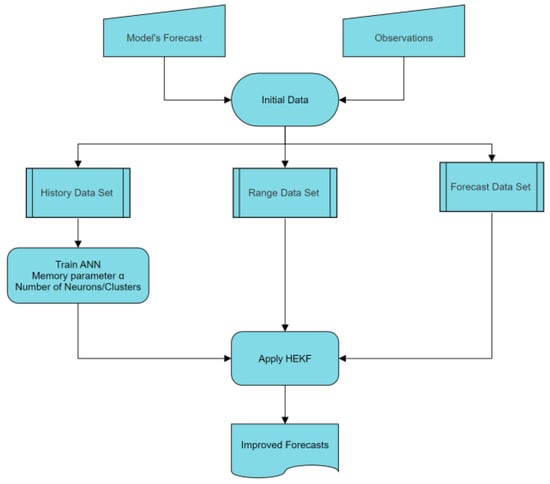
Figure 1.
Method’s Diagram. A combined methodology of EKF and pANNs.
In every stage of the method, both the model’s predictions and the recorded observations are necessary. The forecasts are available from the numerical models WAM and WRF, while the recorded observations were derived from various stations in Greece (Figure 2). Particularly, the wind speed and the temperature observations were obtained from Stations AUTH and AXIOS located on the campus of the Aristotle University of Thessaloniki (AUTH) and the Axios river delta, respectively (Figure 3). On the other hand, the corresponding observations for the significant wave height were obtained from the Heraklion Station in the area of Crete (Figure 4). The key features of each station are summarized in Table 1.
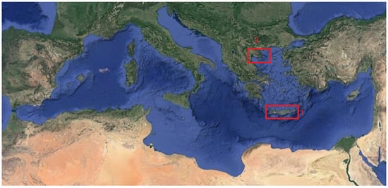
Figure 2.
Mediterranean Sea. Locations of Crete Island (1) and Thessaloniki (2). Region of Greece.
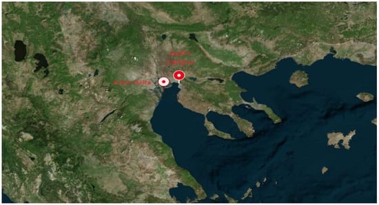
Figure 3.
Locations of AUTH and AXIOS Stations. Thessaloniki.
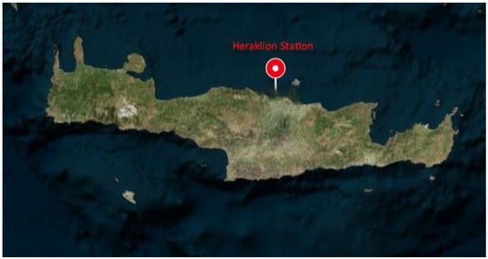
Figure 4.
Location of Heraklion Station. Crete.

Table 1.
Station characteristics.
3. Adaptive Extended Kalman Filter
Kalman Filtering (KF) is a recursive estimation algorithm that produces an improved prediction for an unknown state vector at time , which is given as the information of an observable vector , under the premise that those variables have a linear association. In most real-world applications, though, the model’s dynamics are nonlinear, thus necessitating a different filtering strategy. One such approach is the Extended Kalman Filter, which is a Kalman Filter extension that uses Taylor’s approximation for linearization [38].
To set the framework for the construction of the EKF, consider a nonlinear system characterized by the following state measurement model:
where and are Gaussian nonsystematic parts of the model error with covariance matrices and , respectively, while and are nonlinear, time dependent transition functions. The state space model of Equations (2) and (3) is linearized around the previous or most current state estimate, which can be either the priori estimate or the posteriori estimate , thereby depending on the functional being considered. However, if the linearization process fails to approximate the linear model accurately, the EKF may diverge [39].
More specifically, the EKF includes the following stages:
- Definitions. Jacobian matrices of the nonlinear transition functions.
- Initialization. For , set
- Iteration. For , compute the following:
- Prediction Step:
- Correction Step:
where . The is the Kalman Gain and is the filter’s most essential parameter, since it determines how the filter will respond to any potential changes [40]. For instance, in the case that the value of the Kalman Gain is modest, this can be considered as an indication that the uncertainty in the measurements is high; thus, only a small fraction of the observation will be used to predict the new state.
A challenging issue in Kalman filtering is the choice of the covariance matrices, as a poor selection might substantially impair its performance or possibly lead the filter to diverge. Some researchers have employed fixed covariance matrices that are estimated before the application of the algorithm [41,42], whereas others have altered them during the process, thus utilizing the last seven values of and [14,43,44].
3.1. Residual-Based Method
This work, however, adopts an approach based on the study of Shahrokh and Huang [45], who proposed an estimating method for adaptably adjusting the covariances matrices by applying a constant (memory) parameter .
In every step of the filtering process, the covariance matrix can be estimated using the following formula:
where is the covariance matrix of the innovation, which expresses the difference between the actual measurement and its predicted value based on . is a matrix, while is a vector, with being the dimension of the state vector . One the other hand, is a square matrix, where its size depends on the dimension of the measurement vector .
However, Equation (4) does not guarantee that will be positive, as it should be as a covariance matrix; hence, the residual-based adaptive approach is used to ensure positivity. More specifically, the innovation covariance matrix is approximated as follows:
where , and is the residual. The residual is determined as the difference between the measurement’s actual value and its projected value based on . Therefore, the measurement noise covariance matrix can be computed by the following:
To implement (4), the expectation operation is estimated by averaging itself, and also—instead of the moving window—a memory factor, , is utilized. Hence, the Equation (5) is transformed to the following:
3.2. Innovation-Based Method
During the EKF implementation, the process noise can be found through the following formula:
Thus, using the prediction step, the expected process noise can be defined as follows:
where expresses the measurement innovation. Therefore, an approximation of the process noise covariance matrix can be computed using the following equation:
Similar to the residual-based method, the expectation operation is estimated by averaging itself, and the same memory factor is introduced to adaptively compute the variable over time, thus using the following formula:
Equations (6) and (7) are linear expressions of the parameter that dictate the degree of effect of the prior and subsequent condition. In particular, if the value of the parameter is close to 1, earlier predictions gain more weight, which forces the covariance matrix to take longer to adapt to changes. In their study [45], the value of the (memory) parameter was chosen to be fixed and equal to 0.3.
Τhe selection of the memory parameter, however, cannot be specified without taking into consideration the available data, as critical information required for the study of dynamical systems is lost. To this end, the proposed study implements parametrized Artificial Neural Networks to define that parameter. More thoroughly, the parametrized ANNs are trained for various values of the parameter , and the optimal one is selected to update the covariances matrices based on Equations (6) and (7).
4. Artificial Neural Networks
Artificial Neural Networks are supervised Machine Learning algorithms that draw inspiration from the process of the human brain, thus aiming to discover the fuzzy association between independent input variables and their corresponding dependent targets. The ANNs consist of processing elements, also known as nodes (neurons), and connections. Nodes have their input, which is transformed through a transfer function into output, thus allowing them to communicate with other nodes and to process information to the entire structure. Following how information travels into the network, various ANNs can be constructed [46]. This paper, however, focuses on Feedforward Neural Networks and Radial Basis Function Neural Networks, thus evaluating and comparing their properties as parameter estimators.
4.1. Parametrized Feedforward Neural Networks
Feedforward Neural Networks are artificial models that map input data sets to corresponding outputs and usually consist of multiple layers and neurons that are fully connected in a direct graph. This study presents a three-layer FFNN with one hidden layer of the log-sigmoid function, , as an activation function [47] and one linear output layer.
The proposed parametrized Feedforward Neural Network (Figure 5) accepts an input vector , where , which contains the value of the parameter , along with previous predictions of the numerical weather model, and produces an estimation for the recorded observation at the time . More specifically, is the total number of the available input vectors, and is the size of the model’s previous predictions.
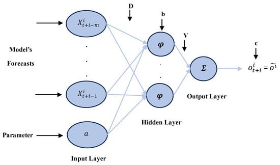
Figure 5.
A three-layer parametrized Feedforward Neural Network.
The pFFNN can be trained for various values of that parameter, thus determining which one best portrays the correlation between the input vector and the related output. Here, we choose . Furthermore, as the size of the network is not specified, the suggested structure is also trained for a number of neurons ranging from 5 to 12.
The main objective of this process is to determine the ideal combination of neurons and the value of the (memory) parameter that optimizes the network’s performance, i.e., that minimizes the Mean Squared Error (MSE):
where is the training error between the th target () and the corresponding output from the pFFNN . Here, is a matrix, with being the size of the input vector, i.e., , and being the number of neurons in the hidden layer. Additionally, and are matrices, while is a scalar.
The determination of these variables is known as the “training” or “learning” stage and is carried out through optimization techniques that seek to minimize the MSE [48]. Several optimization algorithms have been utilized for training ANNs [49,50]. However, regarding the pFFNN’s training, this work implements the Levenberg–Marquardt (LM) method, as the number of the network’s variables is relatively small and also because the MSE is used as a performance index [51].
The Levenberg–Marquardt algorithm combines the steepest descent method with the Gauss–Newton algorithm to update the weights of the network during the training process. To be more precise, the updating rule in the iteration is given by the following formula [52]:
In this case, we have the following:
- is a column vector that contains all the network’s variables (weights and biases).
- is the Jacobian matrix.
- express the vectorized training error, i.e., .
- The quantity represents an approximation of the Hessian matrix introduced by the LM, i.e., .
- is the identity matrix.
- is a combination parameter that takes only positive values and ensures the reversibility of the matrix.
Calculating the Jacobian is a critical factor for the LM implementation, as it can become a difficult and time-consuming procedure due to the complexity of the network’s structure (the number of neurons and hidden layers). The corresponding Jacobian matrix for the proposed parametrized FFNN has the following form:
wherein this case, we have the following:
- express the synaptic weight between the input and the neuron in the hidden layer. Here, , and .
- and are the bias of the neuron and the corresponding synaptic weight between this neuron and the output layer.
- and , with being the input of the neuron based on the training pattern, i.e., , where is the input of the input vector.
- and , where is the bias of the output layer.
When the Jacobian matrix is calculated, the training process (Figure 6) for the pFFNN can be described by the next diagram [52].
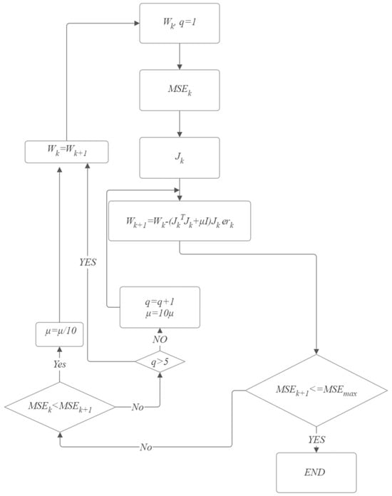
Figure 6.
Training process based on the Levenberg-Marquardt.
Beyond the training algorithm, another aspect to take into account is overfitting. Overfitting is a phenomenon that occurs when an ANN memorizes the characteristics of the training data set, thus preventing thereby the creation of models that effectively generalize from observed data to unseen data [53]. To address this issue, this study applies the early stopping strategy [54]. During the learning process, the training data set is used to update the network’s weights at each epoch, and afterward, the network’s performance is calculated on the validation data set. If the computed error increases for several epochs, the training process is stopped, and the weights that produced the minimum validation error are the optimal network’s variables (Figure 7). The overfitting handle is a crucial part of the training process.
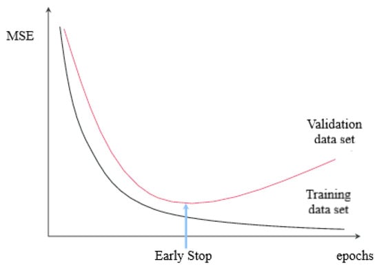
Figure 7.
Early stopping strategy.
To summarize the above procedure, for identifying the optimal combination of neurons and memory parameter , the following tables present the major elements of the suggested network (Table 2), together with Algorithm 1.
Table 2.
Basic elements of the parametrized Feedforward Neural Network.
| Algorithm 1: pFFNN | ||||||||||||
| Create the training data based on History data: | {Inputs, Targets} → {Model’s Forecast, Observations} | |||||||||||
| for do | ||||||||||||
| Insert parameter into the Input data | ||||||||||||
| for each Neuron do | ||||||||||||
| Create the network. % number of neurons, initial values for the weights and biases, number of epochs (total and for Early Stop). | ||||||||||||
| while train ≤ maxtrain % For every network, conduct multiple trainings | ||||||||||||
| Split the Input data randomly, and create the Train and the Validation data sets. | ||||||||||||
| Train network using Levenberg–Marquardt backpropagation algorithm and Early Stop. | ||||||||||||
| performance → Network’s performance % MSE. | ||||||||||||
| if performance < Initial Value | ||||||||||||
| Initial Value → performance | ||||||||||||
| Store the best results for each combination. Number of neurons, performance, parameter, train time. | ||||||||||||
| endif | ||||||||||||
| train → train + 1 | ||||||||||||
| endwhile | ||||||||||||
| train → 1 | ||||||||||||
| endfor | ||||||||||||
| readjust Initial Value | ||||||||||||
| endfor | ||||||||||||
| Define the optimal parameter and number of neurons | ||||||||||||
| if multiple indices in the Total MSE vector show similar results %, their absolute difference is below a threshold position → the index with minimum train time else position → the index with minimum MSE end | ||||||||||||
| Best Neurons → Neuron (position) and Best Parameter → parameter (position) | ||||||||||||
4.2. Parametrized Radial Basis Function Neural Networks
A major drawback of the application of Feedforward Neural Networks is the gradient-based training algorithms that significantly increase the computational cost. Therefore, a different network structure is necessary. On such architecture is the Radial Basis Function Neural Network [55], which represent a unique type of ANN and have been extensively utilized in various applications [56,57,58] due to their simple, straightforward configuration and training algorithms that are characterized by high accuracy and low computational cost [59].
This study presents a parametrized RBF NN consisting of an input layer, one hidden layer with a Gaussian , radial basis transfer functions [47,60,61], and one linear output layer, as illustrated in Figure 8.
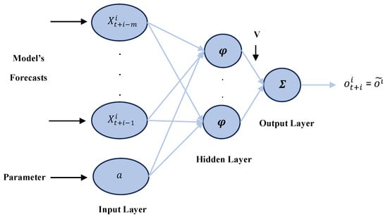
Figure 8.
A parameterized Radial Basis Function Neural Network.
Unlike the corresponding pFFNN structure, which conducts an inner product operation between the weights and the input and adds a bias, pRBF NN computes the Euclidean distance between the input vector and each weight and multiplies the bias. Hence, the so-called net input for the neuron in the hidden layer is calculated as follows:
where expresses the Euclidean distance. The weight acts as the center point of the th node, while the corresponding offset variable , also known as the width, scales the Gaussian distribution, thus instigating it to stretch or compress. The calculated input is then transformed through the activation function and produces the neuron’s output. Each output is multiplied by the corresponding synaptic weight (), and their sum generates the network’s direct response:
where number represents the total number of centers.
In RBF NN modeling, the selection of centers and widths is critical for their successful implementation. More specifically, it is important to define well-distributed centers through the network’s inputs and biases that allow for high overlap among the basis functions. A common established approach for identifying the centers of an RBF network is the k-means++ clustering technique [62].
The k-means++ algorithm is a modification of the k-means [63] that ensures the finding of a set of centers that achieves a approximation for the ideal center set [64]. However, k-means++ does not automatically dictate the ideal number of clusters, as their number must be specified before the usage of the method; thus, it is difficult to define their optimal size.
To avoid this issue and determine the network’s size, the suggested parametrized RBF NN is trained for several clusters ranging from 10 to 70. Furthermore, as the network receives an input vector , it can also be trained for various values of the memory parameter specifying the combination that maximizes the network’s performance, i.e., that minimizes the Sum Squared Error (SSE):
When the centers are established, the width of each neuron cluster can be computed using the following strategy: For each neuron, locate the input vectors from the training set that are closest to the associated center and then compute the average distance between the center and its neighbors [51]:
where and are the closest and the next-closest input vectors to the center . Then, the corresponding width is calculated by the following formula:
After the estimation of the hidden nodes and their widths, the linear interconnection of the hidden and output layer permits the use of linear regression techniques for weight calculation rather than gradient descent approaches [65]. To illustrate the training procedure, let us represent the network’s response for all input vectors in Equation (7) as follows:
where is the output matrix of the radial functions , and is the vector of synaptic weights that connect the hidden layer with the output layer. Hence, the vector of weights that minimizes the SSE is given by the following:
with being the column vector of the measured target values, i.e., .
As in the case of pFFNNs, the risk of overfitting remains high; therefore, the way to deal with it is crucial for the creation of an RBF network with enhanced generalization capabilities. More specifically, the weight decay or ridge regression strategy [66] is utilized instead of early stopping. The goal of this approach is to constrain the magnitude of network weights rather than the quantity of them by adding a parameter in the Sum-Squared Error, which penalizes large weights. Based on this amendment, the SSE (9) is transformed to the following:
The described process is summarized by the following tables, which present the key elements of the proposed pRBFNN (Table 3), as well as Algorithm 2.
Table 3.
Basic elements of the parametrized Radial Basis Function Neural Network.
| Algorithm 2: pRBFNN | ||||||||||||
| Create the training data based on History data: | {Inputs, Targets} → {Model’s Forecast, Observations} | |||||||||||
| for do | ||||||||||||
| Insert parameter into the Input data | ||||||||||||
| for each Cluster do | ||||||||||||
| Create the network. % number of clusters, regularization parameter λ = 0.06. | ||||||||||||
| while train ≤ maxtrain % For every network, conduct multiple trainings | ||||||||||||
| Split the Input data randomly, and create the Train and the Validation data sets. | ||||||||||||
| Define the Centers from the Train data set using K-means++ algorithm, and calculate the widths. Train network using LLS. | ||||||||||||
| performance → Network’s performance % SSE. | ||||||||||||
| if performance < Initial Value | ||||||||||||
| Initial Value → performance | ||||||||||||
| Store the best results for each combination. Number of clusters, performance, parameter, train time. | ||||||||||||
| endif | ||||||||||||
| train → train + 1 | ||||||||||||
| endwhile | ||||||||||||
| train → 1 | ||||||||||||
| endfor | ||||||||||||
| readjust Initial Value | ||||||||||||
| endfor | ||||||||||||
| Define the optimal parameter and number of clusters | ||||||||||||
| if multiple indices in the Total SSE vector show similar results %, their absolute difference is below a threshold position → the index with minimum train time else position → the index with minimum SSE end | ||||||||||||
| Best Clusters → Cluster (position) and Best Parameter → parameter (position) | ||||||||||||
5. Hybrid Extended Kalman Filter
Aiming to improve the predictions of the numerical weather and wave prediction models, the Hybrid Extended Kalman Filter is utilized to decode the forecast error, which is defined as the difference between the recorded observation and the corresponding model’s forecast (For) [17]. In particular, a nonlinear function is considered based on the model’s previous estimation, which in time is given by the following:
or
where is the nonlinear correlation, and is the vectorial parameter that needs to be estimated by the hybrid filter. In this work, is expressed as a neural network, which can be an FFNN or an RBF NN; thus, the variable includes the network’s weights and biases. More specifically, if an FFNN is employed, , and , while if an RBF NN is applied, , and , where . Note here that the centers of the hidden nodes are determined before the application of the hybrid filter through the k-means++ algorithm; hence, they are not included in the vector .
Therefore, the Hybrid Extended Kalman Filter is used as a learning rule intending to determine the network’s optimal parameters. Similar modified Extended Kalman Filter algorithms have been frequently utilized as neural network training methods [67,68,69,70] due to their fast and efficient implementation [71]. These approaches are closely connected to sequential versions of the Gauss–Newton algorithm and, unlike the comparable batch variant, they do not need inversion of the approximate Hessian matrix [51].
To illustrate the procedure of the hybrid filter, the state space model must be established. As a measurement equation, the appropriate choice for this study is Equation (10), whereas the selection of the matching state equation is uncertain, as the evolution of the state vector in time is unknown. Hence, we presume that its change would be random and, as a result, we set the system’s nonlinear transition function . Thus, the state measurement model is the following:
After the dynamic system is defined, the Hybrid Extended Kalman Filter conducts the following steps:
- 1.
- Definition. Jacobian matrix of the nonlinear transition function .
- 2.
- Initialization. For , set
- 3.
- Iteration. For , compute the following:
- 3.1.
- Prediction Step:
- 3.2.
- Correction Step:
Update the measurement noise covariance matrix based on (6):
Update the process noise covariance matrix based on (7):
Applying the algorithm outlined in Algorithm 2, we obtain as the estimated systematic error at time of the numerical model in use. This value represents the optimal weights and biases of the selected ANN, which produces a direct output added to the model’s forecast for time , thus resulting in a more accurate prediction:
Note here that, during the training process, is a column vector; therefore, each variable of the network should be adapted accordingly. Furthermore, the size of the network is determined based on Algorithms 1 and 2 correspondingly. The hybrid filter’s procedure is summarized in Algorithm 3.
| Algorithm 3: Hybrid Extended Kalman Filter | ||
| and the number of hidden notes: | Algorithm 1 or Algorithm 2 | |
| Create the training data set for the Hybrid Filter based on the Range data: | {Inputs, Targets} → {Model’s Forecast, Observations} | |
| % if Algorithm 2 is used, then the centers C are determined by k-means++: | ||
| Create the initial values for the Filter: | ||
| for each training data do | ||
| Implement Hybrid Extended Kalman Filter; % if Algorithm 2 is used, then take the absolute value of the widths (b). | ||
| end | ||
| Create the forecasting data based on the Forecast data: | {Inputs, Targets} → {Model’s Forecast, Observations} | |
| Compute the Improved Forecasts | ||
6. Time Window Process
This section presents a time window process application for the various environmental parameters under study. Specifically, the proposed methodology was applied for Significant Wave Height forecasts concerning the area of Heraklion in 2007–2009 and for Wind Speed and Temperature forecasts concerning the Thessaloniki region in 2020. The aim of this procedure was dual. On the one hand, the stability of the suggested hybrid Filter was tested over different regions and time periods, while on the other hand, the utilized ANNs topologies were compared through their computational cost.
Each time window applies Algorithms 1–3 based on specified history data sets and forecasting intervals, which are defined prior to the usage of the method. These hyper-parameters were not randomly selected but were determined via multiple sensitivity tests, and the results are shown in Table 4.
Table 4.
Time Window Process hyperparameters.
Studying the above, it is clear that there is not a fixed history data set for the ANN’s training that meets all environmental parameters, and the same goes for the predicting intervals. However, that is not the case regarding the hybrid filter’s training, as the conducted tests show that the optimal value for the number of observations is equal to 72. The proposed Time Window Process is described by the Algorithm 4.
| Algorithm 4: Time Window Process | ||
| Load the data: | {Inputs, Targets} → {Model’s Forecast, Observations} | |
| Normalize the data: | {Inputs, Targets} → [–1, 1] | |
| Define the History, the Range, and the Forecast data sets | ||
| Define the maximum number of time windows: | ||
| Initialize the necessary matrix and vectors to store the results | ||
| Define the set of parameters: | → [0:step:1] | |
| Define the set of Neurons or Clusters depending on the ANN structure: | Neuron → [5,...,12] or Cluster→ [10:step1:70] | |
| for | ||
| Training data for the ANN %s one step in time. | ||
| Run the Algorithm 1 or 2 | Obtain the optimal parameter and network size. | |
| → | Training data for the HEKF. | |
| → | Forecasting data for the improved predictions and the evaluation. | |
| Run the Algorithm 3 Denormalize the data | Apply HEKF, and obtain the optimal vector and improved forecasts. Improved forecasts, corresponding model’s forecasts, and recorded observations. | |
| Evaluate the method based on and store the results | Bias, RMSE, and Ns indices. Store Time Series, parameter, and network’s size. | |
| end | ||
| Store the aggregate results from every time window | ||
6.1. Evaluation of the Method
The following metrics were employed to assess the method’s efficacy for the different environmental parameters:
- which serves as a measure of variations between observations and model forecasts, is defined as follows:
- RMSE stands for the Root Mean Squared Error and is a metric that quantifies the error variability by describing the model’s overall predictive behavior, and it is computed by the following equation:
- NS, or the Nash–Sutcliffe model efficiency coefficient, varies between and 1. A perfect match between the model’s forecasts and observations is indicated by a value of 1, but a zero value indicates that the model’s accuracy is only equal to that of the reference model, which in this case is the mean value of the observations . The value of NS is defined as follows:
For every indicator, Forecast is the range of the forecasting interval (number of valid pairs with predictions–observations), expresses the observed value at time , and is the improved prediction of the proposed method, or the model’s forecast, at the same time.
6.2. Results
The results derived from the suggested approach are presented in this section. More specifically, the following Table 5, Table 6 and Table 7 present the average values of the evaluation indicators obtained from the various time windows, while the following time series diagrams present the corresponding time series diagrams. In addition, for every case study, the produced computational cost for each ANN structure is provided. Detailed results from each time window are presented in Appendix A, Appendix B and Appendix C.
Table 5.
Evaluation indicators. Average results for the area of Crete. Significant Wave Height.
Table 6.
Evaluation indicators. Average result for the area of Thessaloniki. Wind speed.
Table 7.
Evaluation indicators. Average results for the area of Thessaloniki. Temperature.
6.2.1. Results Derived from the Crete Region: Heraklion Station—Significant Wave Height
The results from the Crete region show that the suggested methodology improved the predictions of the WAM-cycle 4 numerical model considerably. In particular for 2007, the hybrid filter based on the FFNN produced better results, as the minimum enhancement noticed was 36% and concerned the RMSE index, while the corresponding improvement based on the RBFNN structure was only 11%. Similar conclusions can be extracted by studying the time series diagram (Figure 9—Crete 2007), as the FFNN’s improved forecasts satisfactorily describe the distribution of recorded observations.
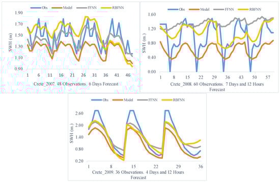
Figure 9.
Time Window Process. Crete 2007–2009. Significant Wave Height.
Moving on to the next period, it is unclear which combination offered the best outcomes. The highest improvement reported was 86% in the Bias index after implementing the FFNN structure, while the biggest enhancements noticed for the RMSE and NS were 24% and 23%, respectively, through the RBFNN. Similar indications can be obtained from the time series diagram (Figure 9—Crete 2008), as the application of the hybrid filter, based on both structures, produced outputs closer to the recorded observations; thus, it is uncertain which architecture is the proper choice. However, if the time efficiency (Figure 10) is taken into consideration, then the RBFNN is the suitable selection, as its computational cost was almost 32 s.
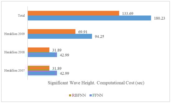
Figure 10.
Computational costs for the ANNs. Crete 2007–2009. Significant wave height.
During 2009, the RBFNN was the optimal choice, since it improved all the evaluation indicators noticeably and also because the FFNN structure produced lower-quality outcomes compared to the model. That can be seen, additionally, through the time series (Figure 9—Crete 2009), where the implementation of the RBFNN hybrid filter led to an adequate convergence of the modeled PDFs to the observations.
6.2.2. Results Derived from the Thessaloniki Region: Stations AUTH and AXIOS—Wind Speed
The results derived from the Thermaikos Gulf, regarding the wind speed, showed that the hybrid filter based on the FFNN improved the forecasts of the WRF model greatly. More specifically, in Station AUTH, the Bias index decreased by 86%, while the values of the RMSE and NS indicators enhanced by 47% and 75%, respectively. Moreover, the distribution of improved predictions (Figure 11—AUTH) exhibited the same tendency, as their morphology in a range of 72 observations was identical to that of the recorded observations. The first time corresponds to the 6th forecast hour (due to WRF model spin-up), and the following times are in hourly intervals (the same applies to the air temperature diagrams).
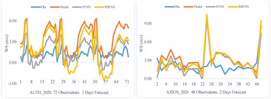
Figure 11.
Time Window Process. Thessaloniki 2020. Wind speed.
On the other hand, the improvement at Station AXIOS was less significant. In this scenario, the Bias dropped by 56%, but the RMSE and NS improved only by 7% and 21%, respectively. The same pattern is visible in the time series diagram (Figure 11—AXIOS), as between the 27th and 48th observation, the improved forecasts failed to approximate the distribution of the recorded observations successfully. Furthermore, it should be noted that the consistent behavior of the FFNN hybrid filter considerably rose the computational cost (Figure 12) of the procedure, since the total time was 53.4 s, whereas the corresponding time for the RBFNN was 15 s.
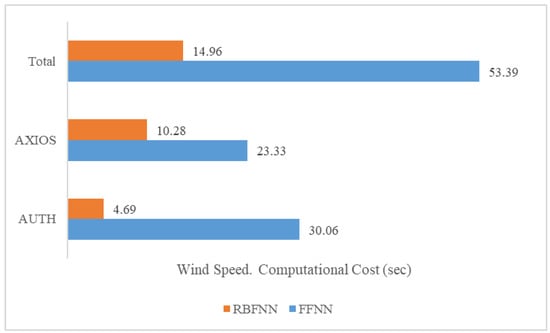
Figure 12.
Computational costs for the ANNs. Thessaloniki 2020. Wind speed.
6.2.3. Results Derived from the Thessaloniki Region: Stations AUTH and AXIOS—Temperature
The implementation of the proposed approach for the environmental parameter of temperature considerably boosted the forecasting capabilities of the WRF model. Studying the time series diagrams (Figure 13) from Stations AUTH and AXIOS, it is observed that, once more, the hybrid filter based on the FFNN generated estimations that matched the available observation perfectly. Additionally, the enhancement noticed in the assessment indicators is of the same magnitude. Particularly, in Station AUTH, the Bias index showed the highest improvement of 98%, while the RMSE showed the lowest improvement of 55%. The corresponding indicators at station AXIOS improved by 99% and 62%, respectively, while the NS index enhanced by 83%. Although, it should be highlighted here that the selection of the FFNN hybrid filter caused a major decrease in the time efficiency of the process, since the total computational cost (Figure 14) exceeded 78 s.
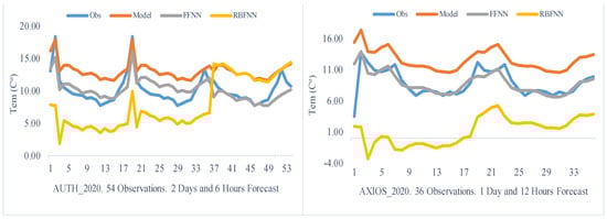
Figure 13.
Time Window Process. Thessaloniki 2020. Temperature.
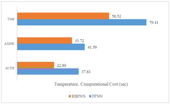
Figure 14.
Computational costs for the ANNs. Thessaloniki 2020. Temperature.
7. Conclusions
A hybrid optimization model for various environmental forecasts has been proposed in this study by utilizing an Extended Kalman Filter enhanced by parametrized Artificial Neural Networks. The suggested system seeks the following:
- To eliminate the systematic forecast error in the direct outputs of the Numerical Weather and Wave Prediction models WRF and WAM;
- To reduce the remaining nonsystematic part of the error and the related forecast uncertainty.
The initial objective was achieved by the implementation of the Extended Kalman Filter, as well as the second goal by the parametrized Artificial Neural Networks. More thoroughly, two different ANN structures were used to define an exogenous parameter, which was employed by the EKF to adaptively estimate the process noise and the measurement noise covariance matrices.
The proposed model was evaluated through a Time Window Process for Significant Wave Height forecasts obtained from the numerical wave model WAM and for wind speed and temperature forecasts derived from the numerical non-hydrostatic system WRF. For each case study, a Feedforward Neural Network and a Radial Function Neural Network were trained for various values of that parameter based on a specified history data set, and the optimal one was selected. Afterward, the Hybrid Extend Kalman Filter was applied, using the selected parameter, to produce improved forecasts for the environmental parameter under study.
The obtained results showed that the suggested hybrid filter greatly improved the statistics of the weather numerical models. Specifically, the systematic errors recorded were practically eliminated, as the Bias index decreased at a percentage of more than 75%, while the RMSE indicator and, therefore, the associated forecast uncertainty was reduced by almost 35%. Moreover, in most case studies, the hybrid filter based on the FFNN structure produced more consistent and balanced final forecasts compared to the corresponding RBFNN’s predictions; thus, it can be considered as an optimal architecture. However, it should be noted that the FFNN’s selection worsened the time efficiency of the system, since the overall computational cost exceeded 320 s.
Furthermore, the Hybrid Extended Kalman Filter based on parametrized ANNs exhibited a stable behavior independent of forecasting horizons and environmental parameters, thus avoiding the limitations of traditional Kalman Filters, which replace initial systematic deviations with similar over- and underestimation periods, thus resulting in reduced mean error values but no significant increase in predictions.
Overall, the combined application of Artificial Neural Networks and Extended Kalman Filters managed to enhance the predictive capacity of the NWWP models in use, regardless of the environmental parameter under study, thus providing a reliable and effective tool for improving weather forecasts. In future stages, the suggested hybrid model can be expanded to similar simulations in domains like economy and biology, where the optimization afforded by the Hybrid Extended Kalman Filter can aid to tailor predictions to specific demands.
Author Contributions
Conceptualization, A.D., G.G. and I.T.F.; methodology, A.D., G.G. and I.T.F.; software, A.D. and I.T.F.; validation, A.D., G.G. and I.T.F.; formal analysis, A.D., G.G. and I.T.F.; investigation, A.D., G.G. and I.T.F.; resources, G.G. and I.P.; data curation, A.D., G.G. and I.P.; writing—original draft preparation, A.D. and I.T.F.; writing—review and editing, A.D., G.G., I.P. and I.T.F.; visualization, A.D., G.G. and I.T.F.; supervision, G.G. and I.T.F.; project administration, G.G. and I.T.F. All authors have read and agreed to the published version of the manuscript.
Funding
This research received no external funding.
Institutional Review Board Statement
Not applicable.
Informed Consent Statement
Not applicable.
Data Availability Statement
Due to privacy the data presented in this study are available on request from the corresponding author.
Conflicts of Interest
The authors declare no conflicts of interest.
Appendix A. Time Window Process for the Crete Region: Significant Wave Height
Table A1.
Time Window Process. Aggregate results—Heraklion 2007. Significant Wave Height.
Table A1.
Time Window Process. Aggregate results—Heraklion 2007. Significant Wave Height.
| Heraklion_2007 | TimeWindow1 | TimeWindow3 | |||||
|---|---|---|---|---|---|---|---|
| Bias | RMSE | NS | Bias | RMSE | NS | ||
| Model | 0.2126 | 0.2459 | −0.9518 | Model | 0.1988 | 0.2347 | −0.5712 |
| FFNN a = 0.6 | 0.1147 | 0.1660 | 0.1102 | FFNN a = 0.5 | −0.1018 | 0.1599 | 0.2703 |
| RBFNN a = 0.6 | −0.1036 | 0.1751 | 0.0105 | RBFNN a = 0.7 | −0.1915 | 0.2352 | −0.5784 |
| TimeWindow2 | TimeWindow4 | ||||||
| Bias | RMSE | NS | Bias | RMSE | NS | ||
| Model | 0.2172 | 0.2522 | −1.1688 | Model | 0.2106 | 0.2397 | −0.5131 |
| FFNN a = 0.6 | 0.0073 | 0.1261 | 0.4582 | FFNN a = 0.4 | 0.1241 | 0.1677 | 0.2597 |
| RBFNN a = 0.7 | −0.1570 | 0.2095 | −0.4958 | RBFNN a = 0.3 | 0.2142 | 0.2410 | −0.5289 |
Table A2.
Time Window Process. Aggregate results—Heraklion 2008. Significant Wave Height.
Table A2.
Time Window Process. Aggregate results—Heraklion 2008. Significant Wave Height.
| Heraklion_2008 | TimeWindow1 | TimeWindow3 | |||||
|---|---|---|---|---|---|---|---|
| Bias | RMSE | NS | Bias | RMSE | NS | ||
| Model | 0.4132 | 0.4896 | 0.6036 | Model | 0.4035 | 0.4841 | 0.6536 |
| FFNN a = 0.2 | 0.0848 | 0.2977 | 0.8534 | FFNN a = 0.4 | −0.0025 | 0.3535 | 0.8153 |
| RBFNN a = 0.2 | 0.1942 | 0.2763 | 0.8737 | RBFNN a = 0.6 | −0.0952 | 0.4335 | 0.7223 |
| TimeWindow2 | TimeWindow4 | ||||||
| Bias | RMSE | NS | Bias | RMSE | NS | ||
| Model | 0.4082 | 0.4872 | 0.6492 | Model | 0.3640 | 0.4289 | 0.6334 |
| FFNN a = 0.3 | 0.0662 | 0.3553 | 0.8134 | FFNN a = 0.6 | −0.3581 | 0.4875 | 0.5265 |
| RBFNN a = 0.2 | 0.1642 | 0.4075 | 0.7545 | RBFNN a = 0 | 0.1566 | 0.3115 | 0.8066 |
Table A3.
Time Window Process. Aggregate results—Heraklion 2009.Significant Wave Height.
Table A3.
Time Window Process. Aggregate results—Heraklion 2009.Significant Wave Height.
| Heraklion_2009 | TimeWindow1 | TimeWindow3 | |||||
|---|---|---|---|---|---|---|---|
| Bias | RMSE | NS | Bias | RMSE | NS | ||
| Model | 0.4113 | 0.5016 | −0.5369 | Model | 0.3806 | 0.4736 | −0.4831 |
| FFNN a = 0.3 | −0.2614 | 0.4761 | −0.3841 | FFNN a = 0.8 | −0.4065 | 0.5330 | −0.8778 |
| RBFNN a = 1 | −0.1274 | 0.3302 | 0.3343 | RBFNN a = 0.9 | 0.1522 | 0.3486 | 0.1968 |
| TimeWindow2 | TimeWindow4 | ||||||
| Bias | RMSE | NS | Bias | RMSE | NS | ||
| Model | 0.4049 | 0.4960 | −0.5528 | Model | 0.3470 | 0.4386 | −0.3393 |
| FFNN a = 0.8 | −0.3716 | 0.5321 | −0.7871 | FFNN a = 0.9 | −0.4806 | 0.5962 | −1.4753 |
| RBFNN a = 0.6 | −0.2510 | 0.3917 | 0.0315 | RBFNN a = 0.9 | −0.2154 | 0.3290 | 0.2463 |
Appendix B. Time Window Process for AUTH and AXIOS: Wind Speed
Table A4.
Time Window Process. Aggregate results—AUTH and AXIOS 2020. Wind speed.
Table A4.
Time Window Process. Aggregate results—AUTH and AXIOS 2020. Wind speed.
| AUTH | TimeWindow1 | AXIOS | TimeWindow1 | ||||
|---|---|---|---|---|---|---|---|
| Bias | RMSE | NS | Bias | RMSE | NS | ||
| Model | −2.1550 | 2.7626 | −24.8339 | Model | −1.0471 | 2.3148 | −11.4628 |
| FFNN a = 0.1 | −0.3290 | 1.5423 | −7.0515 | FFNN a = 0.9 | −0.0462 | 2.0658 | −8.9260 |
| RBFNN a = 0.8 | −1.8776 | 2.3983 | −18.4692 | RBFNN a = 0.9 | −0.2993 | 2.0404 | −8.6839 |
| AUTH | TimeWindow2 | AXIOS | TimeWindow2 | ||||
| Bias | RMSE | NS | Bias | RMSE | NS | ||
| Model | −2.2204 | 2.8262 | −24.8869 | Model | −1.0454 | 2.3157 | −1.4507 |
| FFNN a = 0.5 | −0.4159 | 1.3936 | −5.2943 | FFNN a = 0.9 | −0.8744 | 2.2460 | −1.3054 |
| RBFNN a = 1 | −0.6819 | 2.3781 | −17.3295 | RBFNN a = 0.6 | −1.0694 | 2.3318 | −1.4849 |
| AUTH | TimeWindow3 | ||||||
| Bias | RMSE | NS | |||||
| Model | −2.2833 | 2.9010 | −31.3249 | ||||
| FFNN a = 0.8 | −0.2100 | 1.5403 | −8.1123 | ||||
| RBFNN a = 1 | 0.2677 | 2.2766 | −18.9072 | ||||
Appendix C. Time Window Process for AUTH and AXIOS: Temperature
Table A5.
Time Window Process. Aggregate results—AUTH and AXIOS 2020. Temperature.
Table A5.
Time Window Process. Aggregate results—AUTH and AXIOS 2020. Temperature.
| AUTH | TimeWindow1 | AXIOS | TimeWindow1 | ||||
|---|---|---|---|---|---|---|---|
| Bias | RMSE | NS | Bias | RMSE | NS | ||
| Model | −2.8967 | 3.1822 | −0.6260 | Model | −3.9761 | 4.4915 | −2.4151 |
| FFNN a = 0.3 | −0.0842 | 1.3202 | 0.7201 | FFNN a = 0.3 | −0.4393 | 2.1347 | 0.2286 |
| RBFNN a = 0.1 | 5.7061 | 5.9973 | −4.7751 | RBFNN a = 0 | 9.4823 | 9.9026 | −15.6005 |
| AUTH | TimeWindow2 | AXIOS | TimeWindow2 | ||||
| Bias | RMSE | NS | Bias | RMSE | NS | ||
| Model | −2.8572 | 3.1474 | −0.6865 | Model | −3.5111 | 3.6015 | −3.2669 |
| FFNN a = 0 | −0.9950 | 1.6531 | 0.5348 | FFNN a = 0.2 | 0.4533 | 0.9212 | 0.7208 |
| RBFNN a = 0.8 | 4.2424 | 4.5336 | −2.4991 | RBFNN a = 0 | 5.9151 | 6.0213 | −10.9270 |
| AUTH | TimeWindow3 | ||||||
| Bias | RMSE | NS | |||||
| Model | −3.0722 | 3.2473 | −4.3121 | ||||
| FFNN a = 0.8 | 0.8853 | 1.3748 | 0.0479 | ||||
| RBFNN a = 1 | −3.1368 | 3.3002 | −4.4867 | ||||
References
- Famelis, I.T. Runge-Kutta Solutions for an Environmental Parameter Prediction Boundary Value Problem. J. Coupled Syst. Multiscale Dyn. 2014, 2, 62–69. [Google Scholar] [CrossRef]
- Famelis, I.T.; Galanis, G.; Ehrhardt, M.; Triantafyllou, D. Classical and Quasi-Newton Methods for a Meteorological Parameters Prediction Boundary Value Problem. Appl. Math. Inf. Sci. 2014, 8, 2683–2693. [Google Scholar] [CrossRef]
- Famelis, I.T.; Tsitouras, C. Quadratic shooting solution for an environmental parameter prediction problem. FJAM 2015, 91, 81–98. [Google Scholar] [CrossRef]
- Galanis, G.; Emmanouil, G.; Chu, P.C.; Kallos, G. A New Methodology for the Extension of the Impact of Data Assimilation on Ocean Wave Prediction. Ocean. Dyn. 2009, 59, 523–535. [Google Scholar] [CrossRef]
- Kariniotakis, G.N.; Pinson, P. Evaluation of the MORE-CARE Wind Power Prediction Platform. Performance of the Fuzzy Logic Based Models. In Proceedings of the EWEC 2003—European Wind Energy Conference, Madrid, Spain, 16–19 June 2003. [Google Scholar]
- Kariniotakis, G.; Martí, I.; Casas, D.; Pinson, P.; Nielsen, T.S.; Madsen, H.; Giebel, G.; Usaola, J.; Sanchez, I. What Performance Can Be Expected by Short-Term Wind Power Prediction Models Depending on Site Characteristics? In Proceedings of the EWC 2004 Conference, Tokyo, Japan, 2–4 August 2004; pp. 22–25. [Google Scholar]
- Vanem, E. Long-Term Time-Dependent Stochastic Modelling of Extreme Waves. Stoch. Environ. Res. Risk Assess. 2011, 25, 185–209. [Google Scholar] [CrossRef]
- Giebel, G. On the Benefits of Distributed Generation of Wind Energy in Europe; VDI-Verlag: Dusseldorf, Germany, 2001. [Google Scholar]
- Resconi, G. Geometry of Risk Analysis (Morphogenetic System). Stoch. Environ. Res. Risk Assess. 2009, 23, 425–432. [Google Scholar] [CrossRef]
- Galanis, G.; Louka, P.; Katsafados, P.; Pytharoulis, I.; Kallos, G. Applications of Kalman Filters Based on Non-Linear Functions to Numerical Weather Predictions. Ann. Geophys. 2006, 24, 2451–2460. [Google Scholar] [CrossRef]
- Kalnay, E. Atmospheric Modeling, Data Assimilation and Predictability, 1st ed.; Cambridge University Press: Cambridge, UK, 2002. [Google Scholar] [CrossRef]
- Pelland, S.; Galanis, G.; Kallos, G. Solar and Photovoltaic Forecasting through Post-processing of the Global Environmental Multiscale Numerical Weather Prediction Model. Prog. Photovolt. 2013, 21, 284–296. [Google Scholar] [CrossRef]
- Vergez, P.; Sauter, L.; Dahlke, S. An Improved Kaiman Filter for Satellite Orbit Predictions. J. Astronaut. Sci. 2004, 52, 359–380. [Google Scholar] [CrossRef]
- Hur, S. Short-Term Wind Speed Prediction Using Extended Kalman Filter and Machine Learning. Energy Rep. 2021, 7, 1046–1054. [Google Scholar] [CrossRef]
- Galanis, G.; Papageorgiou, E.; Liakatas, A. A Hybrid Bayesian Kalman Filter and Applications to Numerical Wind Speed Modeling. J. Wind. Eng. Ind. Aerodyn. 2017, 167, 1–22. [Google Scholar] [CrossRef]
- Louka, P.; Galanis, G.; Siebert, N.; Kariniotakis, G.; Katsafados, P.; Pytharoulis, I.; Kallos, G. Improvements in Wind Speed Forecasts for Wind Power Prediction Purposes Using Kalman Filtering. J. Wind. Eng. Ind. Aerodyn. 2008, 96, 2348–2362. [Google Scholar] [CrossRef]
- Donas, A.; Galanis, G.; Famelis, I.T. A Hybrid Extended Kalman Filter Based on a Parametrized FeedForward Neural Network for the Improvement of the Results of Numerical Wave Prediction Models. Environ. Sci. Proc. 2023, 26, 199. [Google Scholar] [CrossRef]
- Group, T.W. The WAM Model—A Third Generation Ocean Wave Prediction Model. J. Phys. Oceanogr. 1988, 18, 1775–1810. [Google Scholar] [CrossRef]
- Ardhuin, F.; Rogers, E.; Babanin, A.V.; Filipot, J.-F.; Magne, R.; Roland, A.; Van Der Westhuysen, A.; Queffeulou, P.; Lefevre, J.-M.; Aouf, L.; et al. Semiempirical Dissipation Source Functions for Ocean Waves. Part I: Definition, Calibration, and Validation. J. Phys. Oceanogr. 2010, 40, 1917–1941. [Google Scholar] [CrossRef]
- Bidlot, J.-R. Present Status of Wave Forecasting at E.C.M.W.F. In Proceedings of the Workshop on Ocean Waves, Shinfield Park, Reading, 25–27 June 2012. [Google Scholar]
- Skamarock, W.C.; Klemp, J.B.; Dudhia, J.; Gill, D.O.; Liu, Z.; Berner, J.; Wang, W.; Powers, J.G.; Duda, M.G.; Barker, D.M.; et al. A Description of the Advanced Research WRF Model Version 4; UCAR/NCAR: Boulder, CO, USA, 2019. [Google Scholar] [CrossRef]
- Davis, C.A.; Jones, S.C.; Riemer, M. Hurricane Vortex Dynamics during Atlantic Extratropical Transition. J. Atmos. Sci. 2008, 65, 714–736. [Google Scholar] [CrossRef][Green Version]
- Hutchinson, T.A. Global WRF-Based Forecast System. Implementation and Applications, 43rd ed.; American Meteorological Society: Boston, MA, USA, 2015. [Google Scholar]
- Lu, Y.; Deng, Y. Initial Transient Response of an Intensifying Baroclinic Wave to Increases in Cloud Droplet Number Concentration. J. Clim. 2015, 28, 9669–9677. [Google Scholar] [CrossRef]
- Shi, J.J.; Tao, W.-K.; Matsui, T.; Cifelli, R.; Hou, A.; Lang, S.; Tokay, A.; Wang, N.-Y.; Peters-Lidard, C.; Skofronick-Jackson, G.; et al. WRF Simulations of the 20–22 January 2007 Snow Events over Eastern Canada: Comparison with In Situ and Satellite Observations. J. Appl. Meteorol. Climatol. 2010, 49, 2246–2266. [Google Scholar] [CrossRef]
- Powers, J.G.; Klemp, J.B.; Skamarock, W.C.; Davis, C.A.; Dudhia, J.; Gill, D.O.; Coen, J.L.; Gochis, D.J.; Ahmadov, R.; Peckham, S.E.; et al. The Weather Research and Forecasting Model: Overview, System Efforts, and Future Directions. Bull. Am. Meteorol. Soc. 2017, 98, 1717–1737. [Google Scholar] [CrossRef]
- Pytharoulis, I.; Tegoulias, I.; Kotsopoulos, S.; Bampzelis, D.; Karacostas, T.; Katragkou, E. Verification of the Operational High-Resolution WRF Forecasts Produced by WAVEFORUS Project. In Proceedings of the 16th Annual WRF Users’ Workshop, Boulder, CO, USA, 15–19 June 2015. [Google Scholar]
- Androulidakis, Y.; Makris, C.; Kolovoyiannis, V.; Krestenitis, Y.; Baltikas, V.; Mallios, Z.; Pytharoulis, I.; Topouzelis, K.; Spondylidis, S.; Tegoulias, I.; et al. Hydrography of Northern Thermaikos Gulf Based on an Integrated Observational-Modeling Approach. Cont. Shelf Res. 2023, 269, 105141. [Google Scholar] [CrossRef]
- Krestenitis, Y.; Pytharoulis, I.; Karacostas, T.S.; Androulidakis, Y.; Makris, C.; Kombiadou, K.; Tegoulias, I.; Baltikas, V.; Kotsopoulos, S.; Kartsios, S. Severe Weather Events and Sea Level Variability Over the Mediterranean Sea: The WaveForUs Operational Platform. In Perspectives on Atmospheric Sciences; Karacostas, T., Bais, A., Nastos, P.T., Eds.; Springer Atmospheric Sciences; Springer International Publishing: Cham, Switzerland, 2017; pp. 63–68. [Google Scholar] [CrossRef]
- Pytharoulis, I.; Karacostas, T.; Tegoulias, I.; Kotsopoulos, S.; Bampzelis, D. Predictability of intense weather events over northern Greece. In Proceedings of the 95th AMS Annual Meeting, Phoenix, AZ, USA, 4–8 January 2015; Available online: https://ams.confex.com/ams/95Annual/webprogram/Manuscript/Paper261575/Pytharoulis_et_al_AMS2015.pdf (accessed on 19 June 2024).
- Pytharoulis, I.; Karacostas, T.; Christodoulou, M.; Matsangouras, I. The July 10, 2019 Catastrophic Supercell over Northern Greece. Part II: Numerical Modelling. In Proceedings of the 15th International Conference on Meteorology, Climatology and Atmospheric Physics (COMECAP2021), Ioannina, Greece, 26–29 September 2021; pp. 885–890. [Google Scholar]
- Androulidakis, Y.; Makris, C.; Mallios, Z.; Pytharoulis, I.; Baltikas, V.; Krestenitis, Y. Storm Surges and Coastal Inundation during Extreme Events in the Mediterranean Sea: The IANOS Medicane. Nat. Hazards 2023, 117, 939–978. [Google Scholar] [CrossRef]
- Eta-12 TPB. Available online: https://www.emc.ncep.noaa.gov/users/mesoimpldocs/mesoimpl/eta12tpb/ (accessed on 19 June 2024).
- Janjić, Z.I. The Step-Mountain Eta Coordinate Model: Further Developments of the Convection, Viscous Sublayer, and Turbulence Closure Schemes. Mon. Wea. Rev. 1994, 122, 927–945. [Google Scholar] [CrossRef]
- Janjić, Z.I. Comments on “Development and Evaluation of a Convection Scheme for Use in Climate Models”. J. Atmos. Sci. 2000, 57, 3686. [Google Scholar] [CrossRef]
- Iacono, M.J.; Delamere, J.S.; Mlawer, E.J.; Shephard, M.W.; Clough, S.A.; Collins, W.D. Radiative Forcing by Long-lived Greenhouse Gases: Calculations with the AER Radiative Transfer Models. J. Geophys. Res. 2008, 113, JD009944. [Google Scholar] [CrossRef]
- Chen, F.; Dudhia, J. Coupling an Advanced Land Surface–Hydrology Model with the Penn State–NCAR MM5 Modeling System. Part I: Model Implementation and Sensitivity. Mon. Wea. Rev. 2001, 129, 569–585. [Google Scholar] [CrossRef]
- Haykin, S. (Ed.) Kalman Filtering and Neural Networks, 1st ed.; Wiley: Hoboken, NJ, USA, 2001. [Google Scholar] [CrossRef]
- Ribeiro, M.; Ribeiro, I. Kalman and Extended Kalman Filters: Concept, Derivation and Properties. Inst. Syst. Robot. 2004, 43, 3736–3741. [Google Scholar]
- Galanis, G.; Anadranistakis, M. A One-dimensional Kalman Filter for the Correction of near Surface Temperature Forecasts. Meteorol. Appl. 2002, 9, 437–441. [Google Scholar] [CrossRef]
- Homleid, M. Diurnal Corrections of Short-Term Surface Temperature Forecasts Using the Kalman Filter. Wea. Forecast. 1995, 10, 689–707. [Google Scholar] [CrossRef]
- Libonati, R.; Trigo, I.; DaCamara, C.C. Correction of 2 M-Temperature Forecasts Using Kalman Filtering Technique. Atmos. Res. 2008, 87, 183–197. [Google Scholar] [CrossRef]
- Galanis, G.; Chu, P.C.; Kallos, G. Statistical Post Processes for the Improvement of the Results of Numerical Wave Prediction Models. A Combination of Kolmogorov-Zurbenko and Kalman Filters. J. Oper. Oceanogr. 2011, 4, 23–31. [Google Scholar] [CrossRef][Green Version]
- Xu, J.; Xiao, Z.; Lin, Z.; Li, M. System Bias Correction of Short-Term Hub-Height Wind Forecasts Using the Kalman Filter. Prot. Control Mod. Power Syst. 2021, 6, 37. [Google Scholar] [CrossRef]
- Akhlaghi, S.; Zhou, N.; Huang, Z. Adaptive Adjustment of Noise Covariance in Kalman Filter for Dynamic State Estimation. In Proceedings of the 2017 IEEE Power & Energy Society General Meeting, Chicago, IL, USA, 16–20 July 2017; IEEE: Chicago, IL, 2017; pp. 1–5. [Google Scholar] [CrossRef]
- Anderson, J.A. An Introduction to Neural Networks; The MIT Press: Cambridge, MA, USA, 1995. [Google Scholar] [CrossRef]
- Wu, Y.; Wang, H.; Zhang, B.; Du, K.-L. Using Radial Basis Function Networks for Function Approximation and Classification. ISRN Applied Mathematics 2012, 2012, 1–34. [Google Scholar] [CrossRef]
- Stăvărache, G.; Ciortan, S.; Rusu, E. Optimization of Artificial Neural Networks Based Models for Wave Height Prediction. E3S Web Conf. 2020, 173, 03007. [Google Scholar] [CrossRef]
- Bui, N.T.; Hasegawa, H. Training Artificial Neural Network Using Modification of Differential Evolution Algorithm. IJMLC 2015, 5, 1–6. [Google Scholar] [CrossRef]
- Rauf, H.T.; Bangyal, W.H.; Ahmad, J.; Bangyal, S.A. Training of Artificial Neural Network Using PSO With Novel Initialization Technique. In Proceedings of the 2018 International Conference on Innovation and Intelligence for Informatics, Computing, and Technologies (3ICT), Sakhier, Bahrain, 20–21 December 2020; IEEE: Sakhier, Bahrain, 2018; pp. 1–8. [Google Scholar] [CrossRef]
- Hagan, M.T.; Demuth, H.B.; Beale, M.H.; De Jésus, O. Neural Network Design, 2nd ed; Oklahoma State University: Stillwater, OK, USA, 2014. [Google Scholar]
- Yu, H.; Wilamowski, B. Levenberg–Marquardt Training. In Intelligent Systems; Irwin, J., Ed.; Electrical Engineering Handbook; CRC Press: Boca Raton, FL, USA, 2011; pp. 1–16. [Google Scholar] [CrossRef]
- Jabbar, H.K.; Khan, R.Z. Methods to Avoid Over-Fitting and Under-Fitting in Supervised Machine Learning (Comparative Study). In Computer Science, Communication and Instrumentation Devices; Research Publishing Services: Singapore, 2014; pp. 163–172. [Google Scholar] [CrossRef]
- Ying, X. An Overview of Overfitting and Its Solutions. J. Phys. Conf. Ser. 2019, 1168, 022022. [Google Scholar] [CrossRef]
- Du, K.-L.; Swamy, M.N.S. Radial Basis Function Networks. In Neural Networks and Statistical Learning; Springer: London, UK, 2014; pp. 299–335. [Google Scholar] [CrossRef]
- Dey, P.; Gopal, M.; Pradhan, P.; Pal, T. On Robustness of Radial Basis Function Network with Input Perturbation. Neural Comput. Appl. 2019, 31, 523–537. [Google Scholar] [CrossRef]
- Que, Q.; Belkin, M. Back to the Future: Radial Basis Function Network Revisited. IEEE Trans. Pattern Anal. Mach. Intell. 2020, 42, 1856–1867. [Google Scholar] [CrossRef]
- Teng, P. Machine-Learning Quantum Mechanics: Solving Quantum Mechanics Problems Using Radial Basis Function Networks. Phys. Rev. E 2018, 98, 033305. [Google Scholar] [CrossRef]
- Alexandridis, A.; Chondrodima, E.; Sarimveis, H. Radial Basis Function Network Training Using a Nonsymmetric Partition of the Input Space and Particle Swarm Optimization. IEEE Trans. Neural Netw. Learn. Syst. 2013, 24, 219–230. [Google Scholar] [CrossRef]
- Gyamfi, K.S.; Brusey, J.; Gaura, E. Differential Radial Basis Function Network for Sequence Modelling. Expert. Syst. Appl. 2022, 189, 115982. [Google Scholar] [CrossRef]
- Zainuddin, Z.; Pauline, O. Function Approximation Using Artificial Neural Networks. WSEAS Trans. Math. 2008, 7, 333–338. [Google Scholar]
- Arthur, D.; Vassilvitskii, S. K-Means++: The Advantages of Careful Seeding. In Proceedings of the eighteenth annual ACM-SIAM Symposium on Discrete Algorithms, SODA ’07; Society for Industrial and Applied Mathematics: Philadelphia, PA, USA, 2007; pp. 1027–1035. [Google Scholar]
- He, J.; Liu, H. The Application of Dynamic K-Means Clustering Algorithm in the Center Selection of RBF Neural Networks. In Proceedings of the 2009 Third International Conference on Genetic and Evolutionary Computing, Guilin, China, 14–17 October 2009; IEEE: Guilin, China, 2009; pp. 488–491. [Google Scholar] [CrossRef]
- Liang, J.; Sarkhel, S.; Song, Z.; Yin, C.; Yin, J.; Zhuo, D. A Faster k-Means++ Algorithm. arXiv 2022, arXiv:2211.15118. [Google Scholar] [CrossRef]
- Su, S.F.; Chuang, C.C.; Tao, C.W.; Jeng, J.T.; Hsiao, C.C. Radial Basis Function Networks With Linear Interval Regression Weights for Symbolic Interval Data. IEEE Trans. Syst. Man. Cybern. B 2012, 42, 69–80. [Google Scholar] [CrossRef]
- Mark, J. Introduction to Radial Basis Function Networks. 1996. Available online: https://faculty.cc.gatech.edu/~isbell/tutorials/rbf-intro.pdf (accessed on 26 May 2024).
- Chernodub, A. Direct Method for Training Feed-Forward Neural Networks Using Batch Extended Kalman Filter for Multi-Step-Ahead Predictions. In Proceedings of the Artificial Neural Networks and Machine Learning—ICANN 2013, Sofia, Bulgaria, 10–13 September 2013; Mladenov, V., Koprinkova-Hristova, P., Palm, G., Villa, A.E.P., Appollini, B., Kasabov, N., Hutchison, D., Kanade, T., Kittler, J., Kleinberg, J.M., et al., Eds.; Lecture Notes in Computer Science. Springer: Berlin/Heidelberg, Germany, 2013; Volume 8131, pp. 138–145. [Google Scholar] [CrossRef]
- Ciocoiu, I.B. RBF Networks Training Using a Dual Extended Kalman Filter. Neurocomputing 2002, 48, 609–622. [Google Scholar] [CrossRef][Green Version]
- De Lima, D.P. Neural Network Training Using Unscented and Extended Kalman Filter. RAEJ 2017, 1. [Google Scholar] [CrossRef]
- Wang, J.; Zhu, L.; Cai, Z.; Gong, W.; Lu, X. Training RBF Networks with an Extended Kalman Filter Optimized Using Fuzzy Logic. In Intelligent Information Processing III; Shi, Z., Shimohara, K., Feng, D., Eds.; IFIP International Federation for Information Processing; Springer: Boston, MA, USA, 2007; Volume 228, pp. 317–326. [Google Scholar] [CrossRef]
- Puskorius, G.V.; Feldkamp, L.A. Extensions and Enhancements of Decoupled Extended Kalman Filter Training. In Proceedings of the International Conference on Neural Networks (ICNN’97), Houston, TX, USA, 9–12 June 1997; IEEE: Houston, TX, USA, 1997; Volume 3, pp. 1879–1883. [Google Scholar] [CrossRef]


Disclaimer/Publisher’s Note: The statements, opinions and data contained in all publications are solely those of the individual author(s) and contributor(s) and not of MDPI and/or the editor(s). MDPI and/or the editor(s) disclaim responsibility for any injury to people or property resulting from any ideas, methods, instructions or products referred to in the content. |
© 2024 by the authors. Licensee MDPI, Basel, Switzerland. This article is an open access article distributed under the terms and conditions of the Creative Commons Attribution (CC BY) license (https://creativecommons.org/licenses/by/4.0/).