Identification of an Unknown Stationary Emission Source in Urban Geometry Using Bayesian Inference

Abstract

Estimating the parameters of an unidentified toxic pollutant source is crucial for public safety, especially in densely populated urban areas. Implementing source term estimation methods in real-world urban environments is challenging due to complex phenomena and the absence of concentration observational data. This work combines a computational fluid dynamics numerical simulation with the Metropolis–Hastings MCMC algorithm to identify the location and quantify the release rate of an unknown source within the geometry of Augsburg city center. To address the lack of concentration measurements, synthetic observations are generated by a forward dispersion model. The methodology is tested using these datasets, both as directly calculated by the forward model and with added Gaussian noise under different source release and wind flow scenarios. The results indicate that in most cases, both the source location and the release rate are estimated accurately. Although a higher performance is achieved using synthetic datasets without additional noise, high accuracy predictions are also obtained in many applications of noisy measurement datasets. In general, the outcomes demonstrate that the presented methodology can be a useful tool for estimating unknown source parameters in real-world urban applications.

1. Introduction

Air pollution causes several negative impacts on human beings, materials, and ecosystems [1,2]. Emergency incidents involving the release of highly toxic air pollutants have significant consequences for public health and environmental safety. Events such as the nuclear disasters at Chernobyl [3] and Fukushima [4], the chemical industry catastrophes in Bhopal [5] and Seveso [6], and the Sarin release terrorist attack at the Japan metro [7] underscore the critical importance of an immediate response from relevant authorities to protect the population. In densely populated urban areas, the release of hazardous substances can result in devastating outcomes, as a large number of individuals may be exposed to high levels of toxic pollutant concentrations. Source Term Estimation (STE) methodologies are designed to immediately identify the characteristics of the pollution source (such as its location, emission strength, and type of pollutant) to provide first responders with accurate information about the unknown source parameters.

In general, Source Term Estimation (STE) algorithms assess the optimal agreement between the concentrations predicted by an Atmospheric Transport and Dispersion (ATD) model and the concentrations observed from a sensor measurement network. An STE problem can be solved by calculating the source–receptor relationship either through “forward” simulations of the ATD model or using the adjoint method in terms of “backward” simulations. The first approach involves multiple runs of the forward ATD model, setting a different source term in each run, and comparing the simulated concentrations with the observed data. This method is effective when the number of potential source terms is limited and known in advance. However, when no information about the source term is known, the forward approach becomes impractical due to the huge number of simulations required. The computational cost of the forward method can be reduced by using the adjoint approach, which was first applied to an STE problem by Pudykiewicz [8]. This method solves the adjoint advection and diffusion equation only once for each sensor, treating the sensor as a source.

STE applications have been developed and tested using various ATD models. Gaussian models have been extensively employed in previous works [9,10,11,12,13] due to their simplicity and minimal computational demands. Conversely, Computational Fluid Dynamics (CFD) models have been utilized in numerous studies [14,15,16,17,18,19,20] dealing with the complexity of urban environments, owing to their capability to provide accurate predictions for concentration fields even at the street scale level. The vast majority of previous CFD-based STE works have used RANS-calculated averaged fields to solve adjoint equations. CFD-based calculations by Jia and Kikumoto [20] demonstrated that a better solution for source parameter estimation was achieved by solving the adjoint equations using fields derived from transient Large Eddy Simulation (LES) models compared to the averaged fields calculated by steady simulations. However, the utilization of transient LES results demands the storage of a large amount of data in order to calculate the adjoint concentrations. Even though the authors successfully employed a wavelet-based compression technique to mitigate data storage requirements in an application at a wind tunnel urban-like domain, the computational resources needed for LES simulations dramatically increase in cases of complex geometries in real urban applications. Although CFD models have been utilized in several pollutant dispersion applications [21,22], one of the primary limitations of CFD modelling, including RANS, at the urban scale is the considerable computational cost for long-term predictions or operational systems. Numerous prior dispersion modelling applications at the urban scale have spanned temporal periods ranging from hours to days [23,24,25]. To address this challenge, pollutant concentrations in urban environments have been calculated for longer periods, extending to several months, using models without chemical reactions in precalculated CFD simulations with varying inlet wind directions [26,27,28].

Another limitation of STE research in urban environments involves the lack of data related to measurements observed from a single standalone source. Consequently, most of the developed methodologies have been applied in non-real-world scenarios. Many previous studies have been evaluated based on field or wind tunnel experimental datasets. To address the absence of observational data, the developed methodologies can be tested in real-world geometries by utilizing synthetic observations, as demonstrated in previous works [29,30].

Various algorithms and methods have been explored in previous studies for estimating source parameters. The optimization approach, extensively utilized in prior research [14,31,32,33], includes algorithms that assess modelled and observed concentrations using a cost function, the minimization of which determines the optimal combination of source terms, leading to the final estimation. Another category of algorithms employed in STE is rooted in Bayesian inference [16,19,20,34,35,36,37,38], which was initially implemented in an STE context in local scale by Keats et al. [16]. Bayesian algorithms use a likelihood function instead of a cost function, and they express source parameter estimation in terms of Probability Distribution Functions (PDF), unlike optimization algorithms that derive a single parameter value. Furthermore, Bayesian algorithms can incorporate any prior knowledge about source characteristics into their framework. They have been effectively utilized across various scales in STE applications, from local to global, exhibiting variations in their characteristics, such as the likelihood or sampling process employed. Additional details on STE algorithms are available in the literature [39,40,41].

The main goal of this work is to implement an STE methodology based on CFD numerical simulations within the complex geometry of a typical central European city. Therefore, the focus of the current research lies in the development and assessment of an STE model capable of estimating the location and release rate of an unknown source within a real urban environment. For this purpose, Bayesian inference is employed, combined with the Markov Chain Monte Carlo (MCMC) algorithm for the sampling process, aiming to provide solutions for unknown source variables as Probability Distribution Functions (PDF). The open-source CFD software suite OpenFOAM v2112 is utilized to calculate the wind field and turbulence parameters and to resolve the adjoint advection and diffusion equations. The city center of Augsburg in Bavaria, Germany, is chosen as the case study. To address the absence of ground-based in situ measurements, a forward model is used to solve the advection and diffusion equations, thereby deriving pollutant concentrations as synthetic observations at specific positions, indicative of sensor locations. The methodology is applied across several release scenarios of stationary point sources of non-reactive passive pollutant under steady meteorological conditions. Various source location scenarios are investigated under air flow conditions corresponding to two different wind directions. The accuracy of the model in estimating source parameters is evaluated for cases utilizing synthetic observations calculated directly from the forward model, as well as when Gaussian noise is added to the synthetic measurements.

2. Materials and Methods

2.1. Source–Receptor Relationship

The STE problem-solving process relies on comparing the observed pollutant concentrations at the measurement points with the corresponding modelled concentrations calculated from an ATD model. Assuming a stationary point source of a passive scalar located at $(x_s,y_s,z_s)$ with a continuous release rate $q_s$. The transport of the passive scalar within the spatial domain is described by the advection–diffusion equation:

$${\displaystyle \frac{\partial C}{\partial t}}+u_j{\displaystyle \frac{\partial C}{\partial x_j}}-{\displaystyle \frac{\partial }{\partial x_j}}D{\displaystyle \frac{\partial C}{\partial x_j}}=q_s\delta \left(x_s,y_s,z_s\right)$$

(1)

where $C$ represents the concentration of the passive scalar, $u_j=(u,v,w)$ is the vector of the three velocity components in Cartesian coordinates $x_j=(x,y,z)$, $D$ is the turbulent diffusion coefficient, and $\delta (·)$ is the Dirac delta function. The diffusion coefficient can be expressed as the sum of the molecular diffusivity, $D_m$, and the turbulent diffusivity, $D_t$:

$$D=D_m+D_t=D_m+{\displaystyle \frac{v_t}{{Sc}_t}}$$

(2)

where ${Sc}_t$ is the turbulent Schmidt number, and $v_t$ is the eddy viscosity. Under steady meteorological conditions, Equation (1) simplifies to:

$$u_j{\displaystyle \frac{\partial C}{\partial x_j}}-{\displaystyle \frac{\partial }{\partial x_j}}(D_m+{\displaystyle \frac{v_t}{{Sc}_t}}){\displaystyle \frac{\partial C}{\partial x_j}}=q_s\delta \left(x_s,y_s,z_s\right)$$

(3)

The source-receptor relationship describes the sensitivity of concentration to every sensor position given a specific set of source parameters, $s=(x_s,y_s,z_s,q_s)$. By utilizing the forward dispersion model, the source–receptor relationship $r_i$ is calculated for each sensor $i$ as:

$${r\left(s\right)}_i=C{\left(x_s,y_s,z_s,q_s\right)}_i$$

(4)

In cases where the potential source parameters are unknown, meaning that the source could be located anywhere within the spatial domain with any release rate, calculating the source–receptor relationship becomes impractical due to the vast number of equations that need to be solved. To address this issue, the adjoint advection–diffusion equation can be used instead of Equation (3) in general form from the following relationship:

$${\displaystyle \frac{{\partial C}_i^{*}}{\partial t}}+u_j{\displaystyle \frac{{\partial C}_i^{*}}{\partial x_j}}-{\displaystyle \frac{\partial }{\partial x_j}}(D_m+{\displaystyle \frac{v_t}{{Sc}_t}}){\displaystyle \frac{{\partial C}_i^{*}}{\partial x_j}}=p_i$$

(5)

Under steady meteorological conditions Equation (5) can be written as:

$$u_j{\displaystyle \frac{{\partial C}_i^{*}}{\partial x_j}}-{\displaystyle \frac{\partial }{\partial x_j}}(D_m+{\displaystyle \frac{v_t}{{Sc}_t}}){\displaystyle \frac{{\partial C}_i^{*}}{\partial x_j}}=p_i$$

(6)

Equation (6) is solved once to determine the adjoint concentration field $C_i^{*}$ for every sensor $i$, using the sensor as the source with the term $p_i$. In that case, the source–receptor relationship is calculated from the equation:

$${r\left(s\right)}_i={{q_{s}C}^{*}\left(x_s,y_s,z_s\right)}_i$$

(7)

A detailed description of the calculation of the source–receptor relationship based on the adjoint advection–diffusion equation is given by Pudykiewicz [8], as well as in many STE estimation studies [16,17,20].

2.2. Bayesian Inference

Bayesian inference methods used in source reconstruction problems estimate the set of unknown source parameters by incorporating a probabilistic approach into the input data. Assuming a set of measurement data $d$, the probability that the set of parameters $s$ represents the true source parameters with respect to $d$ can be calculated using Bayes theorem:

$$p\left(s|d\right)={\displaystyle \frac{p\left(d|s\right)p\left(s\right)}{p\left(d\right)}}\propto p\left(d|s\right)p\left(s\right)$$

(8)

where $p\left(d|s\right)$ is the likelihood function expressing the probability of observing the values $d$ given the source term $s$, $p\left(s\right)$ is the probability of any prior information about the unknown source parameters $s$, and $p\left(d\right)$, the so-called evidence, is a normalizing parameter that does not depend on $s$ and does not influence the relative probabilities. The term $p\left(s|d\right)$, the posterior probability, is the target variable in source parameters estimation problems.

2.2.1. Likelihood Function

In STE research, the likelihood function describes the probability that receptors will observe a set $d_i$ of measurements given a source term $s$. In practical terms, the likelihood quantifies the difference between the modelled concentrations $r_i\left(s\right)$ and the actual measured concentrations $d_i$ at sensor positions $i$. For a given set of source parameters $s$, the relationship between the modelled concentrations $r_i\left(s\right)$ and the observed concentrations $d_i$ can be expressed as:

$$d_i={r\left(s\right)}_i+e$$

(9)

where $e$ is an important variable in STE that encompasses both the biases of the measurement instrument and the model itself. According to Yee et al. [38], the model error, which is the main contributor to the total error, is difficult to characterize as it originates from complex processes. Therefore, it is common to assume that $e$ follows a specific distribution. Wang et al. [37] compared various assumptions about the error distribution and found no clear superiority among them. In the STE literature [16,18,19,20], the simplest and commonly adopted assumption is that the error $e$ follows a Gaussian distribution with a mean of zero and standard deviation ${\sigma }_i$. In that case, the likelihood function is given as:

$$p\left(d|s\right)\propto exp\left[-{\displaystyle \frac{1}{2}}\sum {\displaystyle \frac{{\left(d_i-{r\left(s\right)}_i\right)}^2}{{\sigma }_i^2}}\right]$$

(10)

2.2.2. Prior Probability

The prior probability serves to incorporate any existing knowledge regarding the characteristics of the source before conducting inference. Prior information can enhance the speed and effectiveness of the inference algorithm [20]. In the present study, it is assumed that no prior knowledge about the source characteristics is available before conducting inference. Additionally, the source parameters (location and release rate) are considered to be independent, meaning the value of one does not influence the other. Consequently, a uniform distribution is adopted to represent the prior knowledge as:

$$p\left(s\right)=constant$$

(11)

Equation (11) indicates that the source can be located anywhere and the release rate can take any value. It is essential to note, however, that the source term must always have a meaningful value. For instance, the source should be located within the computational domain, or the release rate should remain positive throughout the calculations.

2.2.3. Posterior Probability and Sampling Process

By incorporating the likelihood function (Equation (10)) and the prior (Equation (11)) in Equation (8), the posterior probability is formulated as:

$$p\left(s|d\right)\propto p\left(d|s\right)p\left(s\right)\propto exp\left[-{\displaystyle \frac{1}{2}}\sum {\displaystyle \frac{{\left(d_i-r_i\right)}^2}{{\sigma }_i^2}}\right]$$

(12)

The solution to the STE problem can be obtained by solving Equation (12) for every possible source term and estimating the source term that maximizes the posterior probability. This process requires a substantial amount of computational resources. To mitigate this computational cost, a sampling algorithm can be employed. In this research, the Metropolis–Hastings MCMC algorithm [42,43,44] is utilized.

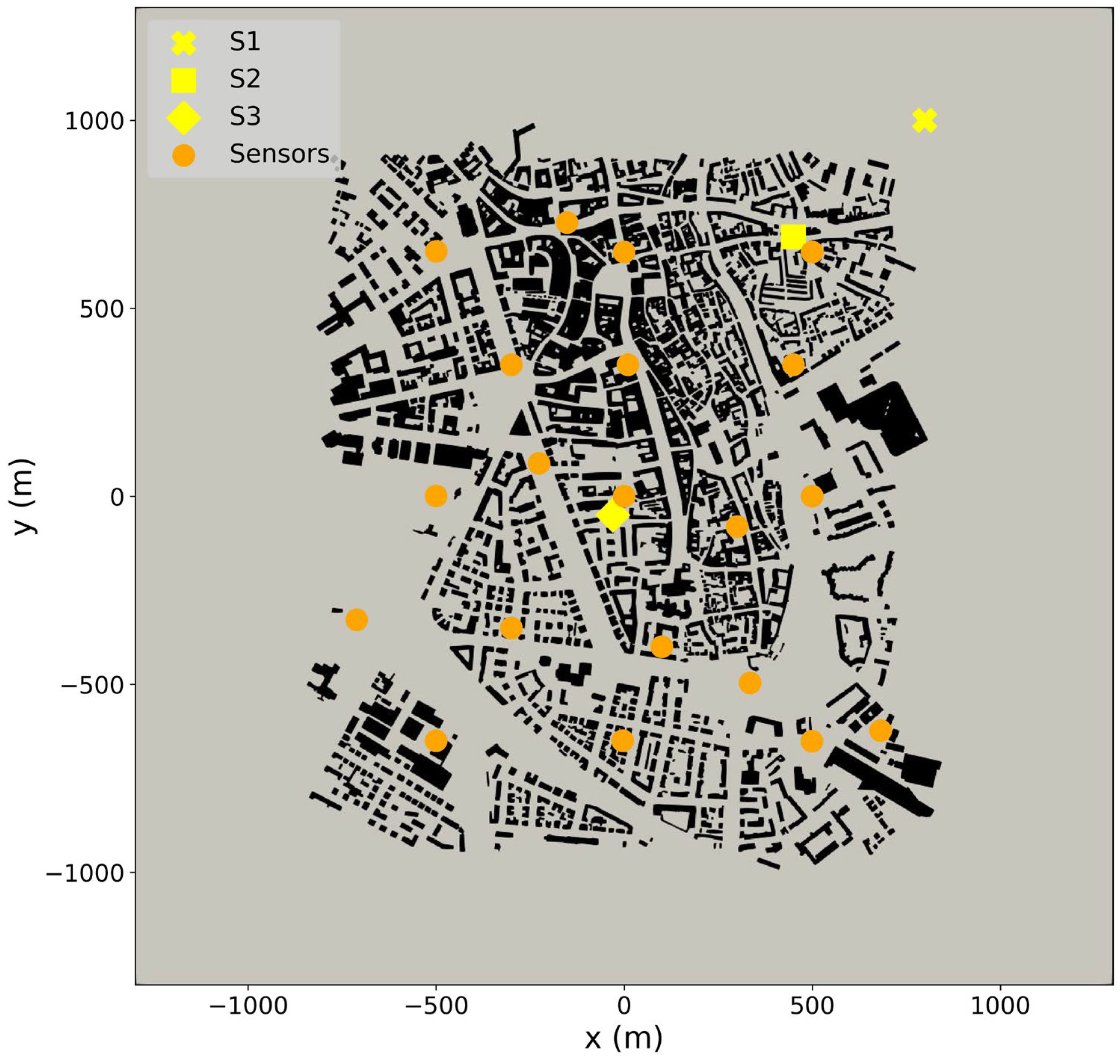
2.3. Case Description

Augsburg is the third largest city in the German state Bavaria, with a population exceeding 300,000 citizens. The broader metropolitan area of Augsburg features significant industrial activity. The complex geometry of Augsburg’s city center and its industrial activities align with the characteristics of the case study that this research aims to investigate.

For the construction of the 3D urban geometry model, information from the open-source tool OpenStreetMap (OSM) [45] is used. OSM is a community-driven software designed for collecting and sharing geographic data. OSM provides both the footprints of 2D geometries and details about building heights. Previous studies [46,47,48] have shown that OSM is capable of competing with commercial providers in offering high-quality data, especially in urban environments. In this work, we assume flat rooftops for the buildings and neglect ventilation structures. These simplifications have been used in urban dispersion modelling [23] and are not expected to significantly affect the accuracy of the simulations. Furthermore, the urban environment’s geometry undergoes a pre-processing step to eliminate inconsistencies in building surfaces. This ensures that the dataset can be utilized for developing the computational mesh without requiring further interferences. The representation of the city’s structure and geometrical characteristics is crucial when developing a CFD model for air quality modelling [49]. Figure 1a visually depicts the domain encompassing the 2 × 1.6 km² study area. The maximum building height ($H_{max}$) within the area of interest is 83.5 m. As illustrated in Figure 1b, the digital domain’s boundaries extend beyond the area of interest, with an upstream distance of 15$H_{max}$, and the height of the domain is set at 6$H_{max}$ [50].

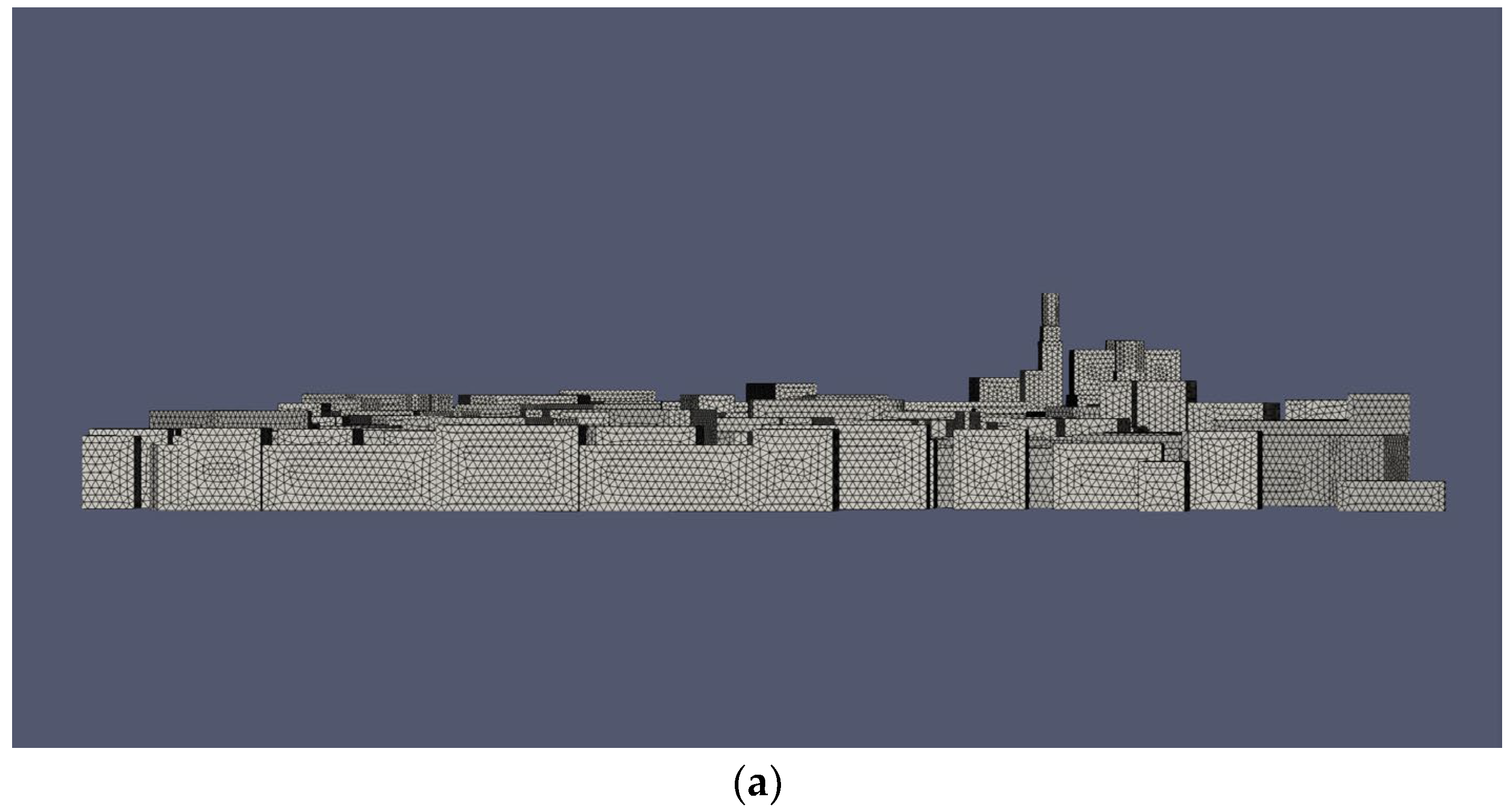
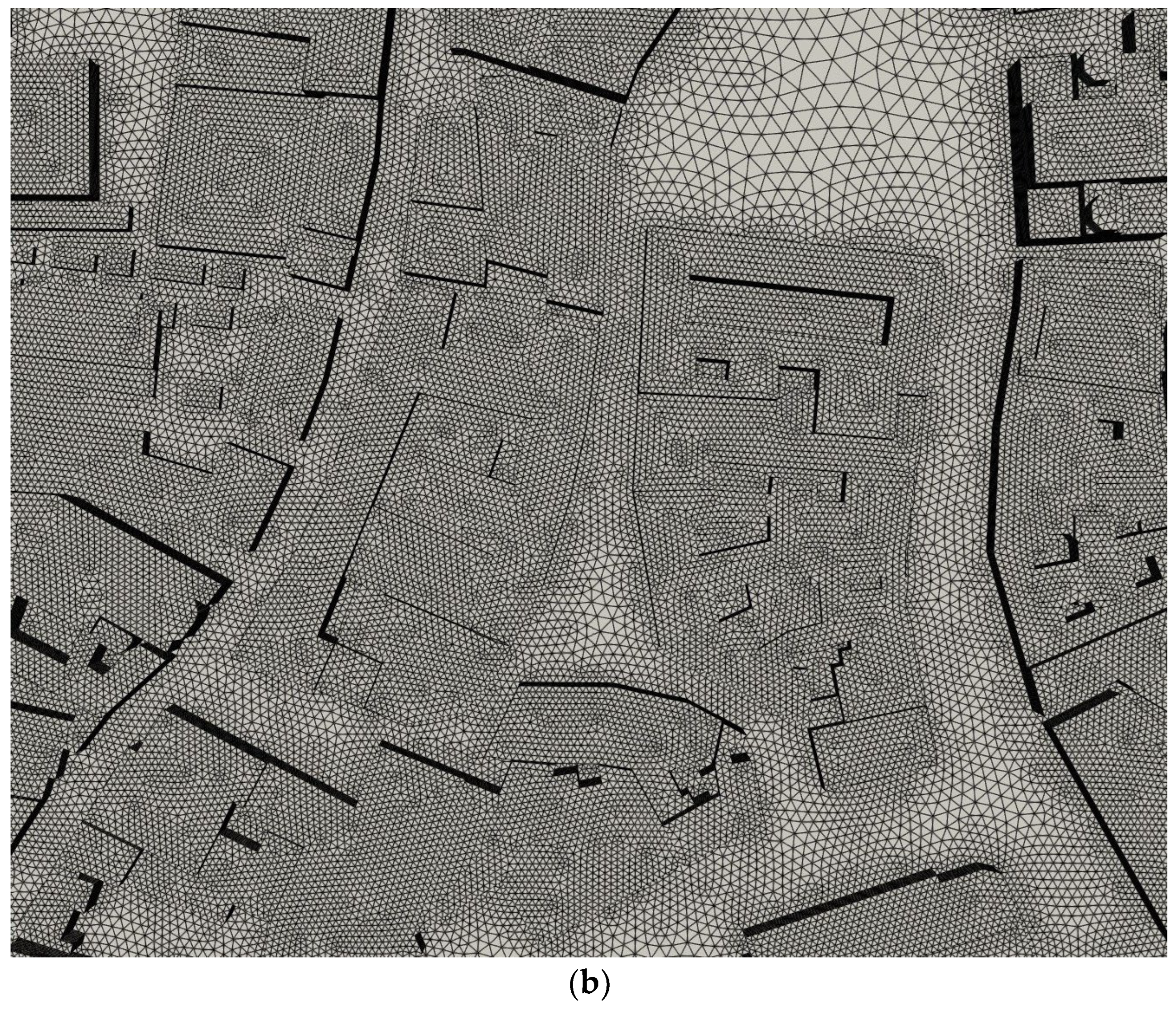
2.3.1. Computational Mesh

A computational mesh is constructed to include the city’s geometrical characteristics. The resolution on the buildings and the ground is 1 m, allowing for high spatial accuracy of the CFD outputs with high refinement in the areas of street canyons. The resolution on the boundaries of the domain is set at 30 m. In Figure 1b is shown the density box that is set around the city is used to set a maximum grid size of 4 m, in order to have higher spatial resolution compared to the rest of the domain in the area of interest containing the buildings. Figure 2a illustrates the mesh in building surfaces of a domain’s neighborhood in the $x-z$ plane, while Figure 2b shows the mesh in the ground and building surfaces in a specific area in the $x-y$ plane. In total, the computational grid consists of 48 million tetrahedral unstructured elements. The dimensionless parameter y⁺, which describes the quality of the mesh at cells near the wall, is calculated for the ground and buildings at a value of 255 and 151, respectively, with an acceptable value lying between 30 and 300 [51].

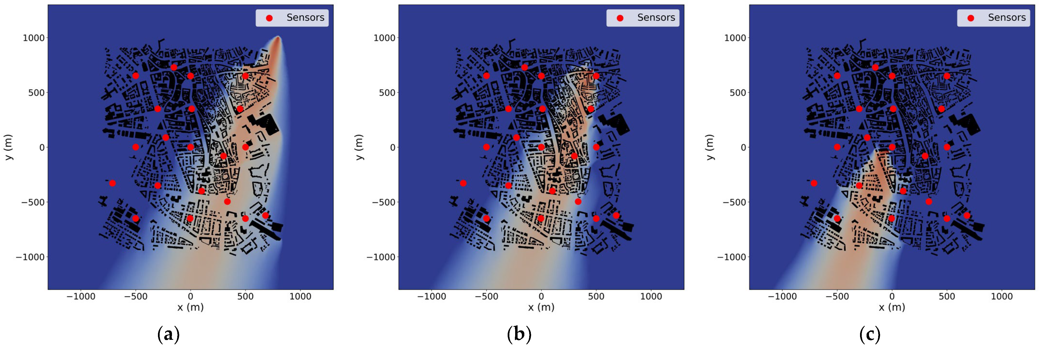
2.3.2. Release Scenarios—Datasets

The absence of actual observations of pollutants emitted by individual sources in the city of Augsburg necessitated the generation of synthetic measurements to facilitate testing of the methodology. Within the defined spatial domain, three different point sources are placed in locations with varying characteristics to assess the accuracy of STE outcomes across different scenarios. Each source is subjected to two different airflow conditions. Specifically, the first source (S1) is positioned outside the building area boundaries but within the computational domain. The second source (S2) is situated in the northeast section of the city within the urban building area. The third source (S3) is placed near the center of the domain at ground level on the $x-y$ plane, also within the urban layout. The altitude for all three sources is at the center of the computational cell closest to ground level, i.e., 2.63 m for S1, 0.12 m for S2, and 0.49 m for S3. The wind flow scenarios are examined using two different wind directions at the inlets: one at 19 degrees and the other at 50 degrees. This investigation encompassed a total of six release scenarios. For generating synthetic observations, 20 positions were chosen within the computational domain to serve as locations for synthetic receptors. All sensor positions are within the urban building area. The altitude of the sensor positions is set at the center of the computational cell closest to 3 m in height. Therefore, the height of the sensors ranges from 1.62 to 4.4 m. Figure 3 illustrates the locations of the three sources marked with yellow (an ‘x’ symbol for S1, a square for S2, and a diamond for S3), and the 20 sensor positions (depicted with dots), in the $x-y$ plane of the spatial domain.

The synthetic measurement data were obtained by performing a CFD simulation for each of the six release scenarios. Using the two wind field scenarios derived from the wind flow model, the forward advection and diffusion equation in steady state (Equation (3)) was applied in each simulation with the corresponding source term for each scenario. Kovalets et al. [17] showed that an error is observed when comparing the source–receptor relationship calculated by the forward model versus the adjoint model. However, this discrepancy is relatively small compared to the actual bias observed between modelled and measured concentrations. Hence, directly using forward concentrations to represent measurements can approximate an almost ideal modelling scenario. To address this issue, Gaussian noise is added to the forward concentrations at sensor locations. The noise for each sensor was generated from a zero-mean Gaussian distribution, and the standard deviation was chosen to ensure that 95% of the distribution resulted in noisy data that varied by no more than a factor of two compared to the non-noisy data. In this study, the STE algorithm was initially applied to synthetic observations from the ideal model (referred to as “non-noisy”), followed by application to synthetic observations with added Gaussian noise (referred to as “noisy”).

2.4. Set Up

2.4.1. Numerical Simulations

As per the methodology, a steady-state CFD simulation is conducted for each wind direction. The average velocity and turbulence viscosity fields obtained from these simulations are utilized to solve both the forward and adjoint advection–diffusion equations. OpenFOAM v2112, an open-source CFD software, is employed for all numerical simulations.

For the wind field simulations, the RANS approach is used together with the standard k-ε turbulence model within the Semi-Implicit Method for Pressure Linked Equations (SIMPLE) solver. To solve Equation (3) (forward model) and Equation (6) (adjoint model), the transport of the passive non-reactive pollutant is calculated by modifying the solver ScalarTransportFOAM for steady-state conditions. Each simulation is conducted with a timestep of 1 s for a duration sufficient to reach steady conditions. The molecular diffusivity, $D_m$, included in Equations (3) and (6), is considered not to influence the dispersion of the passive pollutant, as it is orders of magnitude smaller than the turbulent diffusivity, $D_t$, as evidenced by Henry et al. [52] for a particle dispersion case. Tominaga and Stathopoulos [53] showed that the Schmidt number value, ${Sc}_t$, in Equations (3) and (6) can vary from 0.2 to 1.3. Since investigating the Schmidt number value is beyond the scope of the current study, it is set to 0.7 as suggested by Wang and McNamara [54]. Thermal heat flux effects are considered negligible, and neutral stability conditions are assumed. The strong mean shear from the interaction of the geometry surfaces with the wind flow at an urban scale leads to a much higher contribution of dynamical effects than thermal ones [55]. In such cases, the atmospheric conditions could approximate neutral stability, especially during days of low solar radiation. This assumption has been adopted in previous CFD pollutant dispersion implementations in real environments, providing accurate results [23,24,28]. For neutral stability conditions, the boundary conditions at the inlet can be specified following the equations of Richards and Hoxey [56]. The inflow velocity profile, $U\left(z\right)$, is calculated from Equation (13), where $u^{*}$ is the friction velocity (Equation (14)), $\kappa =0.41$ is the von Karman constant, and $z_0=2 \mathrm{m}$ is the aerodynamic roughness length. The reference velocity, $U_{ref}$, is set to 1 m/s at the reference height, $z_{ref}$, of 3 m.

$$U\left(z\right)={\displaystyle \frac{u^{*}}{\kappa }}ln\left({\displaystyle \frac{z+z_0}{z_0}}\right)$$

(13)

$$u^{*}={\displaystyle \frac{U_{ref}\kappa }{ln\left(\frac{z_{ref}+z_0}{z_0}\right)}}$$

(14)

The turbulent kinetic energy, $k$, and the turbulence dissipation rate, $\epsilon$, at the inlet boundaries are calculated from Equations (15) and (16) [56].

$$k={\displaystyle \frac{{\left(u^{*}\right)}^2}{\sqrt{C_{\mu }}}}$$

(15)

$$\epsilon \left(z\right)={\displaystyle \frac{{\left(u^{*}\right)}^3}{\kappa \left(z+z_0\right)}}$$

(16)

where $C_{\mu }=0.09$ is a model constant.

2.4.2. Metropolis–Hastings MCMC

The Metropolis–Hastings MCMC algorithm was implemented with 100,000 iterations for each case application. A burn-in period of 50,000 samples was initially used, followed by the subsequent 50,000 samples for estimating the posterior distribution. The algorithm initiates from a random point near a sensor observing a concentration higher than a threshold value. The quantity ${\sigma }_i^2$ in Equation (12) is an important variable that represents the allowable error at each sensor. This variable can be independently determined for each sensor, as shown in the literature [16,18]. In this work, we followed the assumption of Jia and Kikumoto [20] that ${\sigma }_i^2=a\times Di$, where $a$ is the constant value across all sensors. For the non-noisy cases, the $a$ value ranges from 0.01 to 0.05, whereas in the noisy cases, it ranges from 0.05 to 0.2.

3. Results

3.1. Synthetic Observations

One important aspect of STE applications is the number of sensors affected by a pollutant source. Here, we present preliminary outcomes of forward simulations used to gather both noisy and non-noisy data. Figure 4a–c and Figure 5a–c illustrate the plumes from three sources under wind directions of 19 and 50 degrees, respectively. The sensor network (marked by red dots) is displayed for each release scenario. The plumes indicate the dispersion of the passive pollutant at a height of 3 m above ground level in the $x-y$ plane. It is important to note that the plumes visualize predicted concentrations above a threshold value, below which concentrations are deemed insignificant for the STE process. This threshold is set at 10⁻¹⁰ kg/m³. For the 19 degrees wind direction scenario, 10 sensors detect concentrations above the threshold from the S1 release (Figure 4a), and the S2 release (Figure 4b). Conversely, the plume from the S3 source (Figure 4c) affects only four sensors, due to S3’s position and the wind direction. The corresponding plumes for the 50 degrees wind direction illustrate that in the S1 scenario (Figure 5a), 13 sensors are impacted by the plume, in the S2 (Figure 5b) case, 10 sensors, and in the S3 (Figure 5c) release, only three sensors detect higher concentrations than the threshold value.

3.2. Source Term Estimation

In this section we present and discuss the results of STE implementation using the Metropolis–Hastings MCMC algorithm. The algorithm is applied independently for both wind directions in each emission scenario, using both noisy and non-noisy synthetic observations, totaling 12 Metropolis-Hastings MCMC runs. The source parameters ($x, y, z$ coordinates of the source location and the release rate $q$) derived as PDFs from the algorithm are compared with the true source parameters to evaluate the algorithm’s accuracy in each scenario. Also, the average values of the PDFs are calculated to provide direct comparisons with the true source parameters.

In Figure 6a,b, the locations of the true and estimated sources for each scenario in the $x-y$ plane within the computational domain are illustrated. Specifically, true sources are marked with red squares, the averaged PDF estimated sources are shown with green dots for the non-noisy data, and with orange “x” symbols for the noisy ones in both 19 degrees (Figure 6a) and 50 degrees (Figure 6b) wind direction. In the 19 degrees case, scenarios S1 and S2 show that both noisy and non-noisy estimates lie near to the true sources. However, for scenario S3, the non-noisy data provide better source location estimates. In the 50 degrees wind direction scenarios, the non-noisy data applications consistently yield better predictions for the estimated source positions across all cases.

Figure 7 presents the Metropolis–Hastings MCMC estimations in the source parameters for the three release scenarios for the 19 degrees wind direction case. The estimations are represented as PDF distributions using histograms for both noisy (in orange) and non-noisy (in grey) data. The average values of the distributions are indicated with a red line for noisy data and a blue line for non-noisy data, while the true source parameters are marked with a green line. Generally, in non-noisy synthetic observation cases, the algorithm yields better estimations, with many parameters closely matching the true values. Moreover, in many cases, the applications using noisy data provide similar predictions compared to those using non-noisy data.

In the S1 scenario (Figure 7a), the average values for the $x$ and $y$ coordinates show that the non-noisy case provides a better solution than the noisy case, and the non-noisy estimation for the $z$ coordinate is slightly more accurate. In the S2 scenario (Figure 7b), both noisy and non-noisy data yield very good estimates for the $x$ and $y$ coordinates, closely matching the true source values, but the $z$ coordinate shows a higher bias in the noisy case. For the S3 scenario (Figure 7c), the non-noisy data provide more accurate estimates for the $x$ and $z$ parameters, while the noisy data yield a more accurate y value. The release rate in non-noisy applications matches the true values across all scenarios, whereas there is a significant discrepancy in the noisy data estimations, particularly in the S2 and S3 scenarios.

In Figure 8, the algorithm’s estimations for the three independent emission scenarios under 50-degree wind direction conditions are illustrated. The noisy dataset shows a broader distribution across many parameters compared to the narrower histograms observed in the non-noisy data. Across all emission cases, particularly in S1 (Figure 8a), the average values of the distributions suggest that the non-noisy applications achieve higher accuracy for horizontal location coordinates ($x$, $y$). Additionally, the noisy data provide predictions comparable to the non-noisy cases, especially in S2 (Figure 8b). In terms of vertical positioning, the estimated $z$ coordinate values from the non-noisy data consistently demonstrate higher algorithmic performance compared to the noisy data. As in the 19 degrees case, far better estimations are observed in S1 compared to S2 and S3 (Figure 8c). Regarding the release rate, both the S1 and S2 scenarios demonstrate high-quality solutions for the non-noisy data application, while the least accuracy is observed in the S3 case.

The results displayed in Figure 7 and Figure 8 provide a visualization of the current STE methodology outcomes in all the investigated cases. However, it is important to quantify these outcomes to evaluate the accuracy of the applied algorithms. For this purpose, the quantities of horizontal distance $R_H$ (Equation (17)), vertical distance $R_V$ (Equation (18)), and the release rate ratio $\mathrm{\Delta }q$ (Equation (19)) between the true ${(x}_t,y_t,z_t,q_t)$ and the mean values of the estimated ${(x}_e,y_e,z_e,q_e)$ distributions are calculated:

$$R_H=\sqrt{{\left(x_e-x_t\right)}^2+{\left(y_e-y_t\right)}^2}$$

(17)

$$R_V=\left|z_e-z_t\right|$$

(18)

$$\mathrm{\Delta }q=\max \left[\left(q_e/q_t\right),\left(q_t/q_e\right)\right]$$

(19)

The target values for the distances $R_H$ and $R_V$ are equal to zero, and for the release rate ratio is unity ($\mathrm{\Delta }q$ = 1).

Table 1. Horizontal distance, vertical distance, and release rate ratio between the true and averaged estimated sources’ parameters for noisy and non-noisy data cases in each wind direction and source location scenario.

Wind Direction	Source	${\mathit{R}}_{\mathit{H}}$ (m)		${\mathit{R}}_{\mathit{V}}$ (m)		$\mathbf{\Delta }\mathit{q}$ (-)
		Non-Noisy	Noisy	Non-Noisy	Noisy	Non-Noisy	Noisy
19 degrees	S1	39.37	82.65	5.85	5.55	1.00	1.08
	S2	22.70	36.90	12.66	21.50	1.04	1.42
	S3	91.06	109.21	24.44	31.59	1.03	2.15
50 degrees	S1	5.19	80.94	2.88	6.11	1.04	1.07
	S2	36.44	59.56	5.22	18.26	1.03	1.16
	S3	109.15	157.92	28.01	57.53	1.46	2.20

presents the calculated horizontal and vertical distances, as well as the release rate ratio between the true and averaged estimated sources for the examined scenarios. Comparing the noisy and non-noisy data cases, it is observed that in most instances, the non-noisy data application yields solutions closest to the target values of $R_H$, $R_V$, and $\mathrm{\Delta }q$. This outcome is anticipated, since the use of directly simulated concentrations from the forward model as synthetic measurements, without adding any noise, suggests an almost ideal model. However, it is noteworthy that there are several instances where the noisy data cases provide solutions comparable to the non-noisy ones. Specifically, for the horizontal distance, there are three cases (S2 and S3 for 19 degrees, and S2 for 50 degrees) where the estimated location for the noisy data is close to the corresponding estimations of the non-noisy data. The vertical distance values indicate that using non-noisy data generally results in estimated positions closer to the true height compared to using noisy data across all cases, except for S1 in the 19-degree scenario. Regarding the release rate ratio values, nearly perfect predictions are observed for the release rate in all non-noisy cases, except for S3 in the 50-degree scenario. Additionally, satisfactory accuracy is also achieved with the use of noisy synthetic measurement data.

To enhance comprehension of the calculated distances within the specific geometry, it is useful to compare the calculated values with a characteristic length of the computational domain’s geometry. Therefore, the maximum building height $H_{max}$ can be used as a reference length against the horizontal and vertical distances.

The values of $R_H$ indicate that, for non-noisy measurements, the applications of S1 and S2 in both wind directions provide a solution where the estimated source has a horizontal distance less than $H_{max}$. In contrast, for the S3 case, the calculated $R_H$ exceeds $H_{max}$. As detailed in Section 3.1, in the two wind conditions examined, the S1 and S2 scenarios show a higher number of sensors (10–13) detecting concentrations above the threshold value compared to S3, where only three (in the 19-degree case) and four (in the 50-degree case) observations surpass the threshold. From this perspective, it is clear that a better solution for horizontal distance is achieved when the pollutant plume influences more sensors in the measurement network. This observation applies similarly to cases involving noisy data, where $R_H$ values are nearly equal to or lower than $H_{max}$ in the S1 and S2 scenarios, but higher in the S3 scenarios.

By examining the vertical distances, it is observed that, in all cases, the calculated values are smaller compared to $H_{max}$, indicating satisfactory accuracy. For each set of synthetic data and wind directions separately, it is noted that the lowest $R_V$ are shown in the S1 cases. This could be attributed to the source location, as depicted in Figure 3, where the S1 position is situated in an open area outside the complex building geometries, unlike S2 and S3, which are located in narrow urban streets. Furthermore, the calculated $R_V$ values appear to be influenced by the number of measurements exceeding the threshold concentration, as noted for $R_H$.

The release rate ratio values demonstrate that, in the ideal model (non-noisy data), when a significant number of sensors detect a concentration above the threshold, the release rate estimation closely matches the true emission rate of the sources. The $\mathrm{\Delta }q$ values for non-noisy S3 in the 50-degree wind direction scenario suggest that reducing the number of observations surpassing the threshold value could affect the discrepancy between estimated and true release rates. For the noisy data cases of S1 and S2, although $\mathrm{\Delta }q$ is higher compared to non-noisy data, it remains close to unity, which is the target. However, the results for S3 indicate a reduced accuracy in noisy data applications when fewer sensors detect the plume. Overall, $\mathrm{\Delta }q$ outcomes demonstrate an acceptable performance, as the estimated release rate values are consistently within the same order of magnitude and close to the true values across all scenarios.

4. Discussion

The findings demonstrate that the applied STE methodology, based on CFD numerical simulations, effectively predicts both source locations and release rates within the complex geometry of a real urban area of a European city in the majority of cases. Figure 7 and Figure 8 show that in almost all the applied scenarios, the true value of the target variable (x, y, z, q) is within the estimated PDF histogram and lies near the average PDF value. The evaluation quantities indicate that, for all scenarios, the average value of the PDF distribution for the source location is within a horizontal distance from the true source that is less than, or very close to, twice the maximum building height. The corresponding distance in the vertical level is consistently less than the maximum building height across all scenarios. The release rate ratio results demonstrate high accuracy in most cases.

The main limitation of this work is the lack of actual measurements in the area of interest. To assess the validity of the Metropolis–Hastings MCMC algorithm in a real-world geometry case, the algorithm is tested using synthetic measurement datasets generated directly by the forward model. These datasets are used both without noise and with added Gaussian noise to simulate the biases from measurement and modelling uncertainties.

Generally, the estimated PDFs (Figure 7 and Figure 8) and the evaluation quantities (Table 1) indicate a higher performance when applying the algorithm to synthetic data without added Gaussian noise. In certain scenarios (S1 and S2 for the 50-degree wind direction), the PDF histograms illustrate wider distributions when noise is introduced, increasing the uncertainty in the source parameter estimations. The improved performance with non-noisy datasets aligns with previous studies [30] and was anticipated, as synthetic observations were derived directly from the forward dispersion model, approaching nearly ideal conditions for the application.

Bayesian-based algorithms can include an estimation of the measurement and modelling bias by adding the variable ${\sigma }_i$ in the calculations of the posterior probability (Equation (12)). In this work, we assume that ${\sigma }_i^2=a\times Di$, where $a$ is a constant value across all sensors, ranging from 0.01 to 0.05 in non-noisy scenarios and from 0.05 to 0.2 in noisy cases. The higher accuracy in non-noisy application may be due to the fact that the observations are directly calculated from the forward model, including only uncertainties from the adjoint equations, contributing to a small total error that is likely similar in each sensor. Conversely, Gaussian noise introduces varying levels of biases in each sensor stochastically. From this point of view, future work should investigate techniques capable of predicting the error in each sensor separately, potentially enhancing the algorithm’s accuracy in such cases.

The algorithm’s validity is demonstrated by achieving acceptable estimations using noisy observation datasets in most scenarios. It is noteworthy that, in certain release scenarios, the noisy observation cases show a performance similar to or slightly better than the non-noisy ones, as shown in Table 1. For example, in the S2 and S3 scenarios at a wind direction of 19 degrees, and in the S2 scenario at 50 degrees, the noisy dataset estimations are close to the non-noisy ones at the horizontal level. Additionally, in the S1 scenario at 19 degrees, the vertical distance between the estimated and true sources is slightly lower in the noisy application than in the non-noisy one. Similar release rate estimations are also achieved for both the noisy and non-noisy datasets in the S1 scenario at 19 degrees, and in the S1 and S2 scenarios at 50 degrees.

The outcomes show that the performance of the STE algorithm is strongly associated with the number of sensors detecting concentrations above the threshold value. This relationship is particularly pronounced in the non-noisy cases, where the accuracy of the results declines when only three or four observations surpass the threshold, as noted in the S3 cases for both release scenarios. Specifically, in Table 1, it is observed that both the horizontal and vertical distances increase in the S3 cases compared to the corresponding values for the S1 and S2 scenarios. A lower accuracy is observed for the release rate ratio only in the S3 case for the 50-degree wind direction. A similar trend is observed in some noisy data applications, although additional uncertainties can affect the method’s performance in these cases. The results in the Efthimiou et al. study [15] show that a better solution can be achieved even by using a network with a lower number of sensors in different source location cases within the same spatial domain under the same meteorological conditions. In our work, it is observed that the accuracy of the estimations is strongly correlated with the number of sensors detecting a concentration above a specified threshold.

The characteristics of the area surrounding the source significantly influence the accuracy of vertical location estimates. Sources located at ground level in open spaces yield better predictions for the $z$ coordinate compared to those placed near the ground in street canyons or among obstacles. These findings are consistent with the work of Efthimiou et al. [15], where the vertical distance between the estimated and true values for a source located in an open space was lower or only slightly higher, compared to scenarios where the sources were within street canyons. At the same time, the open space source scenario provided significantly less accurate estimations for the horizontal location and release rate.

Two important assumptions of the current study are that the pollutant is treated a non-reactive passive substance and that neutral stability atmospheric conditions are assumed, neglecting thermal effects. These assumptions have been successfully adopted in previous STE [18,20] and air quality [23,28] CFD applications, providing accurate results. Incorporating atmospheric chemistry and thermal effects into CFD models increases both the complexity and the computational requirements. In emergency cases involving hazardous airborne releases, rapid response times are crucial for protecting the population. Therefore, future research should focus on STE applications aimed at improving model accuracy by integrating chemical and thermal processes while managing computational demands. To expedite response times, future work should explore the use of precalculated wind and concentration fields within the area of interest.

5. Conclusions

The goal of this work is to estimate the location and release rate of an unknown source within the complex geometry of the Augsburg city center. To achieve this, the Metropolis–Hastings MCMC algorithm is employed to generate probability distribution functions (PDFs) for the source parameters, based on pollutant concentration measurements and concentrations calculated by a CFD model. To address the absence of available measurements, the forward dispersion model is utilized to generate concentrations that are used as synthetic observations in a 20-sensor measurement network. Three different source locations are investigated under two distinct wind direction conditions. The algorithm’s performance in estimating the source parameters is assessed in all scenarios by using the synthetic observations, both as directly calculated by the forward model and with added Gaussian noise.

Overall, the results highlight that the applied methodology is capable of providing accurate solutions for identifying the source location and quantifying the release rate in an urban-scale environment. Moreover, the methodology is successfully implemented in a real-world urban geometry, such as Augsburg’s city center. The findings indicate higher accuracy in the applications of non-noisy synthetic observations, while acceptable solutions are achieved from the algorithm in Gaussian-noisy synthetic measurement cases. This suggests the methodology’s potential use as a supporting tool in emergency situations, providing relevant authorities with valuable information on unknown source characteristics. Future work should focus on evaluating the current methodology against real observation datasets to validate its effectiveness. Furthermore, the use of precomputed fields from numerical simulations should be explored to reduce the high computational demands of CFD models, as rapid response time is crucial in emergency situations.

References

1. Vlachokostas, C.; Achillas, C.; Slini, T.; Moussiopoulos, N.; Banias, G.; Dimitrakis, I. Willingness to Pay for Reducing the Risk of Premature Mortality Attributed to Air Pollution: A Contingent Valuation Study for Greece. Atmos. Pollut. Res. 2011, 2, 275–282. [Google Scholar] [CrossRef]
2. Vlachokostas, C.; Banias, G.; Athanasiadis, A.; Achillas, C.; Akylas, V.; Moussiopoulos, N. Cense: A Tool to Assess Combined Exposure to Environmental Health Stressors in Urban Areas. Environ. Int. 2014, 63, 1–10. [Google Scholar] [CrossRef] [PubMed]
3. Anspaugh, L.R.; Catlin, R.J.; Goldman, M. The Global Impact of the Chernobyl Reactor Accident. Science 1988, 242, 1513–1519. [Google Scholar] [CrossRef] [PubMed]
4. Ohtsuru, A.; Tanigawa, K.; Kumagai, A.; Niwa, O.; Takamura, N.; Midorikawa, S.; Nollet, K.; Yamashita, S.; Ohto, H.; Chhem, R.K.; et al. Nuclear Disasters and Health: Lessons Learned, Challenges, and Proposals. Lancet 2015, 386, 489–497. [Google Scholar] [CrossRef] [PubMed]
5. Chouhan, T.R. The Unfolding of Bhopal Disaster. J. Loss Prev. Process Ind. 2005, 18, 205–208. [Google Scholar] [CrossRef]
6. Pocchiari, F.; Silano, V.; Zampieri, A. Human Health Effects from Accidental Release of Tetrachlorodibenzo-p-Dioxin (tcdd) at Seveso, italy. Ann. N. Y. Acad. Sci. 1979, 320, 311–320. [Google Scholar] [PubMed]
7. Okumura, T.; Takasu, N.; Ishimatsu, S.; Miyanoki, S.; Mitsuhashi, A.; Kumada, K.; Tanaka, K.; Hinohara, S. Report on 640 Victims of the Tokyo Subway Sarin Attack. Ann. Emerg. Med. 1996, 28, 129–135. [Google Scholar] [CrossRef] [PubMed]
8. Pudykiewicz, J.A. Application of Adjoint Tracer Transport Equations for Evaluating Source Parameters. Atmos. Environ. 1998, 32, 3039–3050. [Google Scholar] [CrossRef]
9. Allen, C.T.; Young, G.S.; Haupt, S.E. Improving Pollutant Source Characterization by Better Estimating Wind Direction with a Genetic Algorithm. Atmos. Environ. 2007, 41, 2283–2289. [Google Scholar] [CrossRef]
10. Liu, Y.; Jiang, Y.; Zhang, X.; Pan, Y.; Qi, Y. Combined Grey Wolf Optimizer Algorithm and Corrected Gaussian Diffusion Model in Source Term Estimation. Processes 2022, 10, 1238. [Google Scholar] [CrossRef]
11. Li, H.; Zhang, J.; Yi, J. Computational Source Term Estimation of the Gaussian Puff Dispersion. Soft Comput. 2019, 23, 59–75. [Google Scholar] [CrossRef]
12. Park, M.; Ladosz, P.; Oh, H. Source Term Estimation Using Deep Reinforcement Learning With Gaussian Mixture Model Feature Extraction for Mobile Sensors. IEEE Robot. Autom. Lett. 2022, 7, 8323–8330. [Google Scholar] [CrossRef]
13. Wade, D.; Senocak, I. Stochastic Reconstruction of Multiple Source Atmospheric Contaminant Dispersion Events. Atmos. Environ. 2013, 74, 45–51. [Google Scholar] [CrossRef]
14. Efthimiou, G.C.; Kovalets, I.V.; Venetsanos, A.; Andronopoulos, S.; Argyropoulos, C.D.; Kakosimos, K. An Optimized Inverse Modelling Method for Determining the Location and Strength of a Point Source Releasing Airborne Material in Urban Environment. Atmos. Environ. 2017, 170, 118–129. [Google Scholar] [CrossRef]
15. Efthimiou, G.C.; Kovalets, I.V.; Argyropoulos, C.D.; Venetsanos, A.; Andronopoulos, S.; Kakosimos, K.E. Evaluation of an Inverse Modelling Methodology for the Prediction of a Stationary Point Pollutant Source in Complex Urban Environments. Build. Environ. 2018, 143, 107–119. [Google Scholar] [CrossRef]
16. Keats, A.; Yee, E.; Lien, F.-S. Bayesian Inference for Source Determination with Applications to a Complex Urban Environment. Atmos. Environ. 2007, 41, 465–479. [Google Scholar] [CrossRef]
17. Kovalets, I.V.; Andronopoulos, S.; Venetsanos, A.G.; Bartzis, J.G. Identification of Strength and Location of Stationary Point Source of Atmospheric Pollutant in Urban Conditions Using Computational Fluid Dynamics Model. Math. Comput. Simul. 2011, 82, 244–257. [Google Scholar] [CrossRef]
18. Xue, F.; Kikumoto, H.; Li, X.; Ooka, R. Bayesian Source Term Estimation of Atmospheric Releases in Urban Areas Using LES Approach. J. Hazard. Mater. 2018, 349, 68–78. [Google Scholar] [CrossRef] [PubMed]
19. Xue, F.; Li, X.; Ooka, R.; Kikumoto, H.; Zhang, W. Turbulent Schmidt Number for Source Term Estimation Using Bayesian Inference. Build. Environ. 2017, 125, 414–422. [Google Scholar] [CrossRef]
20. Jia, H.; Kikumoto, H. Source Term Estimation in Complex Urban Environments Based on Bayesian Inference and Unsteady Adjoint Equations Simulated via Large Eddy Simulation. Build. Environ. 2021, 193, 107669. [Google Scholar] [CrossRef]
21. Rapkos, N.; Boikos, C.; Ioannidis, G.; Ntziachristos, L. Direct Deposition of Air Pollutants in the Wake of Container Vessels: The Missing Term in the Environmental Impact of Shipping. Atmos. Pollut. Res. 2024, 15, 102013. [Google Scholar] [CrossRef]
22. Boikos, C.; Rapkos, N.; Ioannidis, G.; Oppo, S.; Armengaud, A.; Siamidis, P.; Tsegas, G.; Ntziachristos, L. Factors Affecting Pedestrian-Level Ship Pollution in Port Areas: CFD in the Service of Policy-Making. Build. Environ. 2024, 258, 111594. [Google Scholar] [CrossRef]
23. Ioannidis, G.; Li, C.; Tremper, P.; Riedel, T.; Ntziachristos, L. Application of CFD Modelling for Pollutant Dispersion at an Urban Traffic Hotspot. Atmosphere 2024, 15, 113. [Google Scholar] [CrossRef]
24. Rivas, E.; Santiago, J.L.; Lechón, Y.; Martín, F.; Ariño, A.; Pons, J.J.; Santamaría, J.M. CFD Modelling of Air Quality in Pamplona City (Spain): Assessment, Stations Spatial Representativeness and Health Impacts Valuation. Sci. Total Environ. 2019, 649, 1362–1380. [Google Scholar] [CrossRef] [PubMed]
25. Rafael, S.; Vicente, B.; Rodrigues, V.; Miranda, A.I.; Borrego, C.; Lopes, M. Impacts of Green Infrastructures on Aerodynamic Flow and Air Quality in Porto’s Urban Area. Atmos. Environ. 2018, 190, 317–330. [Google Scholar] [CrossRef]
26. Parra, M.A.; Santiago, J.L.; Martín, F.; Martilli, A.; Santamaría, J.M. A Methodology to Urban Air Quality Assessment during Large Time Periods of Winter Using Computational Fluid Dynamic Models. Atmos. Environ. 2010, 44, 2089–2097. [Google Scholar] [CrossRef]
27. Santiago, J.L.; Borge, R.; Martin, F.; de la Paz, D.; Martilli, A.; Lumbreras, J.; Sanchez, B. Evaluation of a CFD-Based Approach to Estimate Pollutant Distribution within a Real Urban Canopy by Means of Passive Samplers. Sci. Total Environ. 2017, 576, 46–58. [Google Scholar] [CrossRef] [PubMed]
28. Martín, F.; Janssen, S.; Rodrigues, V.; Sousa, J.; Santiago, J.L.; Rivas, E.; Stocker, J.; Jackson, R.; Russo, F.; Villani, M.G.; et al. Using Dispersion Models at Microscale to Assess Long-Term Air Pollution in Urban Hot Spots: A FAIRMODE Joint Intercomparison Exercise for a Case Study in Antwerp. Sci. Total Environ. 2024, 925, 171761. [Google Scholar] [CrossRef] [PubMed]
29. Haupt, S.E.; Young, G.S.; Allen, C.T. Validation of a Receptor–Dispersion Model Coupled with a Genetic Algorithm Using Synthetic Data. J. Appl. Meteorol. Clim. 2006, 45, 476–490. [Google Scholar] [CrossRef]
30. Allen, C.T.; Haupt, S.E.; Young, G.S. Source Characterization with a Genetic Algorithm–Coupled Dispersion–Backward Model Incorporating SCIPUFF. J. Appl. Meteorol. Clim. 2007, 46, 273–287. [Google Scholar] [CrossRef]
31. Ma, D.; Tan, W.; Zhang, Z.; Hu, J. Parameter Identification for Continuous Point Emission Source Based on Tikhonov Regularization Method Coupled with Particle Swarm Optimization Algorithm. J. Hazard. Mater. 2017, 325, 239–250. [Google Scholar] [CrossRef] [PubMed]
32. Thomson, L.C.; Hirst, B.; Gibson, G.; Gillespie, S.; Jonathan, P.; Skeldon, K.D.; Padgett, M.J. An Improved Algorithm for Locating a Gas Source Using Inverse Methods. Atmos. Environ. 2007, 41, 1128–1134. [Google Scholar] [CrossRef]
33. Wang, Y.; Chen, B.; Zhu, Z.; Wang, R.; Chen, F.; Zhao, Y.; Zhang, L. A Hybrid Strategy on Combining Different Optimization Algorithms for Hazardous Gas Source Term Estimation in Field Cases. Process Saf. Environ. Prot. 2020, 138, 27–38. [Google Scholar] [CrossRef]
34. Ickowicz, A.; Septier, F.; Armand, P.; Delignon, Y. Adaptive Bayesian Algorithms for the Estimation of Source Term in A Complex Atmospheric Release. In Proceedings of the 15th International Conference on Harmonisation within Atmospheric Dispersion Modelling for Regulatory Purposes, Madrid, Spain, 6–9 May 2013. [Google Scholar]
35. Jia, H.; Kikumoto, H. Line Source Estimation of Environmental Pollutants Using Super-Gaussian Geometry Model and Bayesian Inference. Environ. Res. 2021, 194, 110706. [Google Scholar] [CrossRef] [PubMed]
36. Lane, R.O.; Briers, M.; Copsey, K. Approximate Bayesian Computation for Source Term Estimation. In Proceedings of the IMA Conference on Mathematics in Defence Cody Technology Park, Farnborough, Hampshire, UK, 19 November 2009. [Google Scholar]
37. Wang, Y.; Huang, H.; Huang, L.; Ristic, B. Evaluation of Bayesian Source Estimation Methods with Prairie Grass Observations and Gaussian Plume Model: A Comparison of Likelihood Functions and Distance Measures. Atmos. Environ. 2017, 152, 519–530. [Google Scholar] [CrossRef]
38. Yee, E.; Hoffman, I.; Ungar, K. Bayesian Inference for Source Reconstruction: A Real-World Application. Int. Sch. Res. Not. 2014, 2014, 507634. [Google Scholar] [CrossRef] [PubMed]
39. Bieringer, P.E.; Young, G.S.; Rodriguez, L.M.; Annunzio, A.J.; Vandenberghe, F.; Haupt, S.E. Paradigms and Commonalities in Atmospheric Source Term Estimation Methods. Atmos. Environ. 2017, 156, 102–112. [Google Scholar] [CrossRef]
40. Shankar Rao, K. Source Estimation Methods for Atmospheric Dispersion. Atmos. Environ. 2007, 41, 6964–6973. [Google Scholar] [CrossRef]
41. Hutchinson, M.; Oh, H.; Chen, W.H. A Review of Source Term Estimation Methods for Atmospheric Dispersion Events Using Static or Mobile Sensors. Inf. Fusion 2017, 36, 130–148. [Google Scholar] [CrossRef]
42. Gilks, W.R.; Richardson, S.; Spiegelhalter, D. Markov Chain Monte Carlo in Practice; CRC Press: Boca Raton, FL, USA, 1995. [Google Scholar]
43. Metropolis, N.; Rosenbluth, A.W.; Rosenbluth, M.N.; Teller, A.H.; Teller, E. Equation of State Calculations by Fast Computing Machines. J. Chem. Phys. 1953, 21, 1087–1092. [Google Scholar] [CrossRef]
44. Carlin, B.P.; Louis, T.A. Bayes and Empirical Bayes Methods for Data Analysis. Stat. Comput. 1997, 7, 153–154. [Google Scholar] [CrossRef]
45. Haklay, M.; Weber, P. Openstreetmap: User-Generated Street Maps. IEEE Pervasive Comput. 2008, 7, 12–18. [Google Scholar] [CrossRef]
46. Mooney, P.; Corcoran, P.; Winstanley, A.C. Towards Quality Metrics for OpenStreetMap. In Proceedings of the 18th SIGSPATIAL International Conference on Advances in Geographic Information Systems, San Jose, CA, USA, 3–5 November 2010; pp. 514–517. [Google Scholar]
47. Haklay, M. How Good Is Volunteered Geographical Information? A Comparative Study of OpenStreetMap and Ordnance Survey Datasets. Environ. Plan. B Plan. Des. 2010, 37, 682–703. [Google Scholar] [CrossRef]
48. Neis, P.; Zielstra, D.; Zipf, A. The Street Network Evolution of Crowdsourced Maps: OpenStreetMap in Germany 2007–2011. Future Internet 2011, 4, 1–21. [Google Scholar] [CrossRef]
49. Antoniou, A.; Ioannidis, G.; Ntziachristos, L. Realistic Simulation of Air Pollution in an Urban Area to Promote Environmental Policies. Environ. Model. Softw. 2024, 172, 105918. [Google Scholar] [CrossRef]
50. Blocken, B. Computational Fluid Dynamics for Urban Physics: Importance, Scales, Possibilities, Limitations and Ten Tips and Tricks towards Accurate and Reliable Simulations. Build. Environ. 2015, 91, 219–245. [Google Scholar] [CrossRef]
51. Ariff, M.; Salim, S.M.; Cheah, S.C. Wall Y+ Approach for Dealing with Turbulent Flows over a Surface Mounted Cube: Part 2—High Reynolds Number. In Proceedings of the Seventh International Conference on CFD in the Mineral and Process Industries, Melbourne, Australia, 9–11 December 2009. [Google Scholar]
52. Henry, F.; Bonifacio, R.G.M.; Glasgow, L.A. Numerical Simulation of Transport of Particles Emitted from Ground-Level Area Source Using Aermod and CFD. Eng. Appl. Comput. Fluid. Mech. 2014, 8, 488–502. [Google Scholar] [CrossRef]
53. Tominaga, Y.; Stathopoulos, T. Turbulent Schmidt Numbers for CFD Analysis with Various Types of Flowfield. Atmos. Environ. 2007, 41, 8091–8099. [Google Scholar] [CrossRef]
54. Wang, X.; McNamara, K.F. Evaluation of CFD Simulation Using RANS Turbulence Models for Building Effects on Pollutant Dispersion. Environ. Fluid Mech. 2006, 6, 181–202. [Google Scholar] [CrossRef]
55. Sanchez, B.; Santiago, J.L.; Martilli, A.; Martin, F.; Borge, R.; Quaassdorff, C.; de la Paz, D. Modelling NOX Concentrations through CFD-RANS in an Urban Hot-Spot Using High Resolution Traffic Emissions and Meteorology from a Mesoscale Model. Atmos. Environ. 2017, 163, 155–165. [Google Scholar] [CrossRef]
56. Richards, P.J.; Hoxey, R.P. Appropriate Boundary Conditions for Computational Wind Engineering Models Using the K-ε Turbulence Model. Comput. Wind Eng. 1993, 1, 145–153. [Google Scholar] [CrossRef]
Figure 1. Area of interest in Augsburg map (a) and computational domain containing the city’s digital model (b).
Atmosphere 15 00871 g001
Figure 2. Computational mesh (a) in the buildings in the x z plane and (b) in the buildings and ground in the x y plane.
Atmosphere 15 00871 g002aAtmosphere 15 00871 g002b
Figure 3. The locations of the three sources, S1, S2, and S3, are indicated with “x”, square, and diamond symbols, respectively, while the sensors are marked with dots in the x y plane.
Atmosphere 15 00871 g003
Figure 4. Pollutant plumes of S1 (a), S2 (b), and S3 (c) for 19 degrees wind direction in x y plane at 3 m height. The sensors are depicted with red dots.
Atmosphere 15 00871 g004
Figure 5. Pollutant plumes of S1 (a), S2 (b), and S3 (c) for 50 degrees wind direction in x y plane at 3 m height. The sensors are depicted with red dots.
Atmosphere 15 00871 g005
Figure 6. Locations of the true (red squares), estimated non-noisy (green dots), and estimated noisy (orange “x”) sources in the three release cases (S1, S2, S3) at 19 degrees (a) and 50 degrees (b) wind direction in the x y plane.
Atmosphere 15 00871 g006
Figure 7. PDF distributions of the estimated parameters ( x ,   y ,   z ,   q ) in noisy (orange) and non-noisy (grey) applications for 19 degrees wind direction scenarios for S1 (a), S2 (b), and S3 (c) sources. The averaged value of noise (red line) and non-noise (blue line) data cases are illustrated. The values of true source parameters are depicted with a green line.
Atmosphere 15 00871 g007
Figure 8. PDF distributions of the estimated parameters ( x ,   y ,   z ,   q ) in noisy (orange) and non-noisy (grey) applications for 50 degrees wind direction scenarios for S1 (a), S2 (b), and S3 (c) sources. The averaged value of noise (red line) and non-noise (blue line) data cases are illustrated. The values of true source parameters are depicted with a green line.
Atmosphere 15 00871 g008