

Analysis of Different Height Correction Models for Tropospheric Delay Grid Products over the Yunnan Mountains
Abstract
:1. Introduction
2. Method and Data
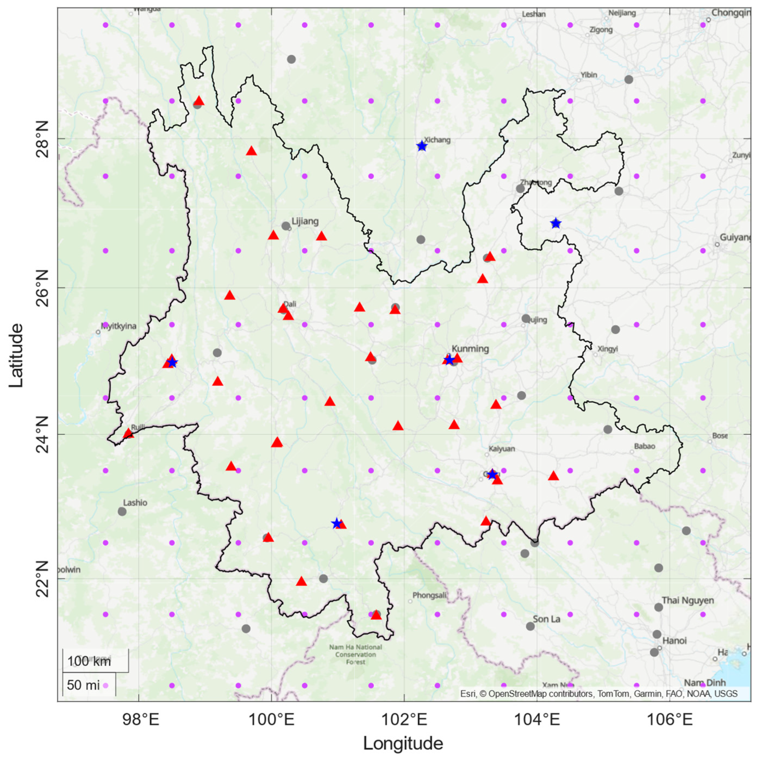
2.1. Data
2.2. The Vertical Reduction Models in ZHD
- -based
- model
- -based
- model
- IGPZWD
2.3. The Vertical Reduction Models in ZWD
- Constant WSH model (CWSH)
3. Results
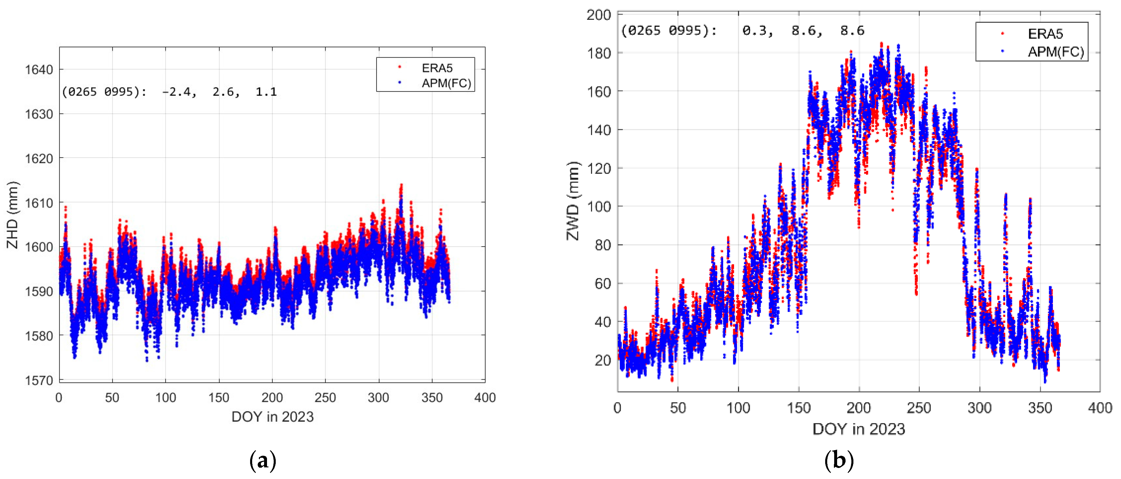
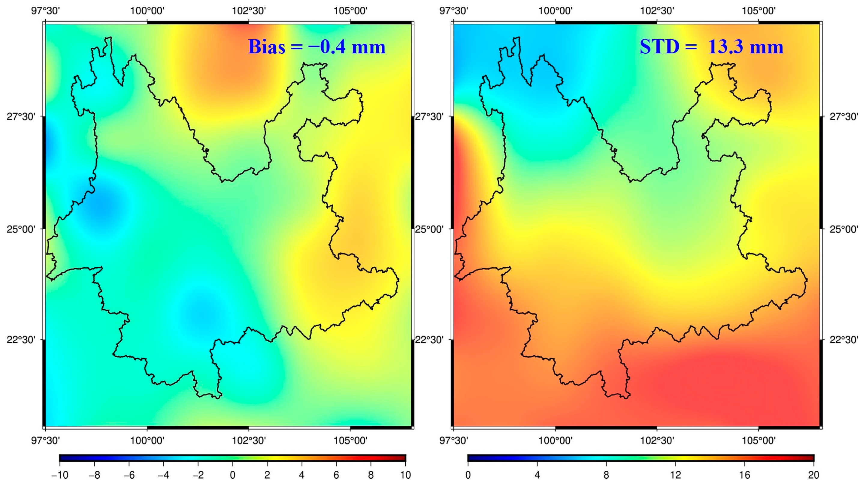
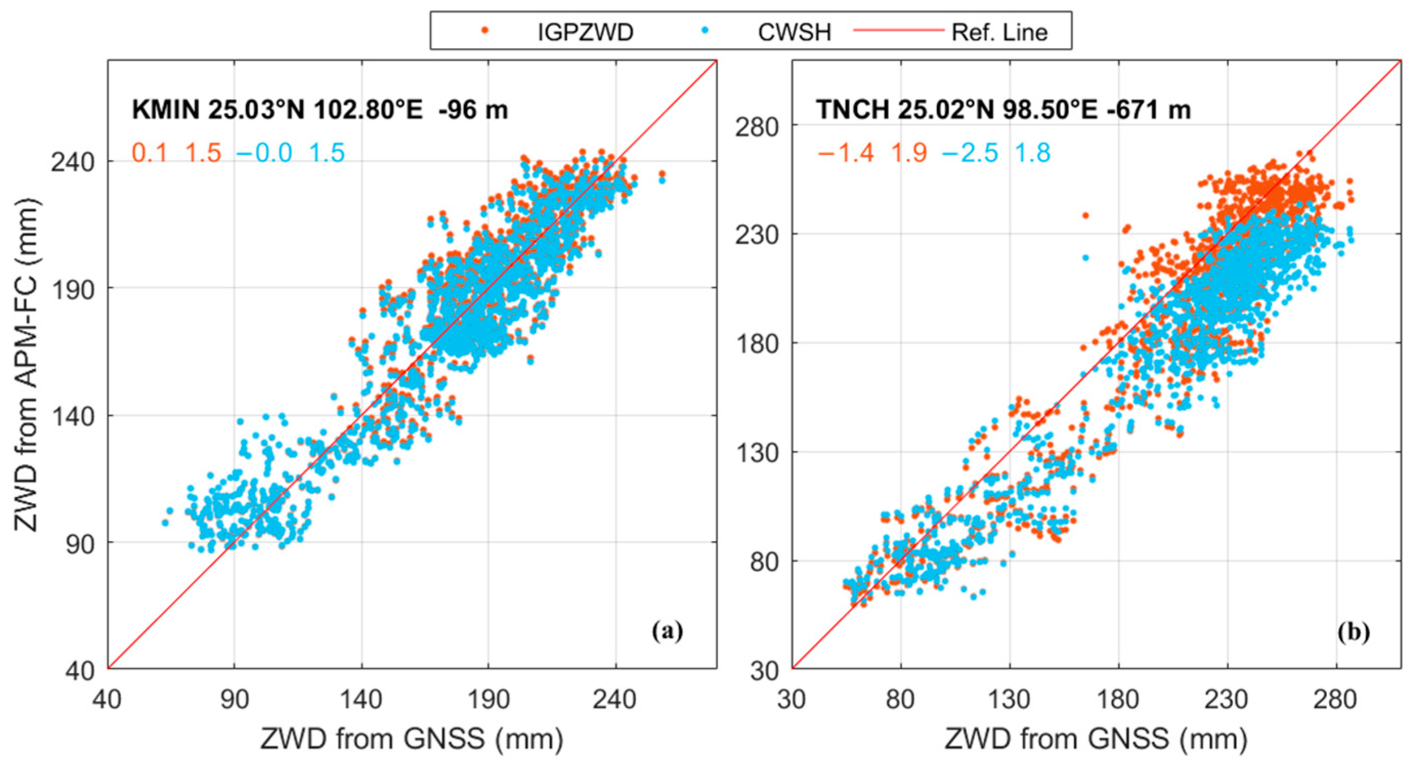
3.1. The ZHD and ZWD Performance from Grid Products
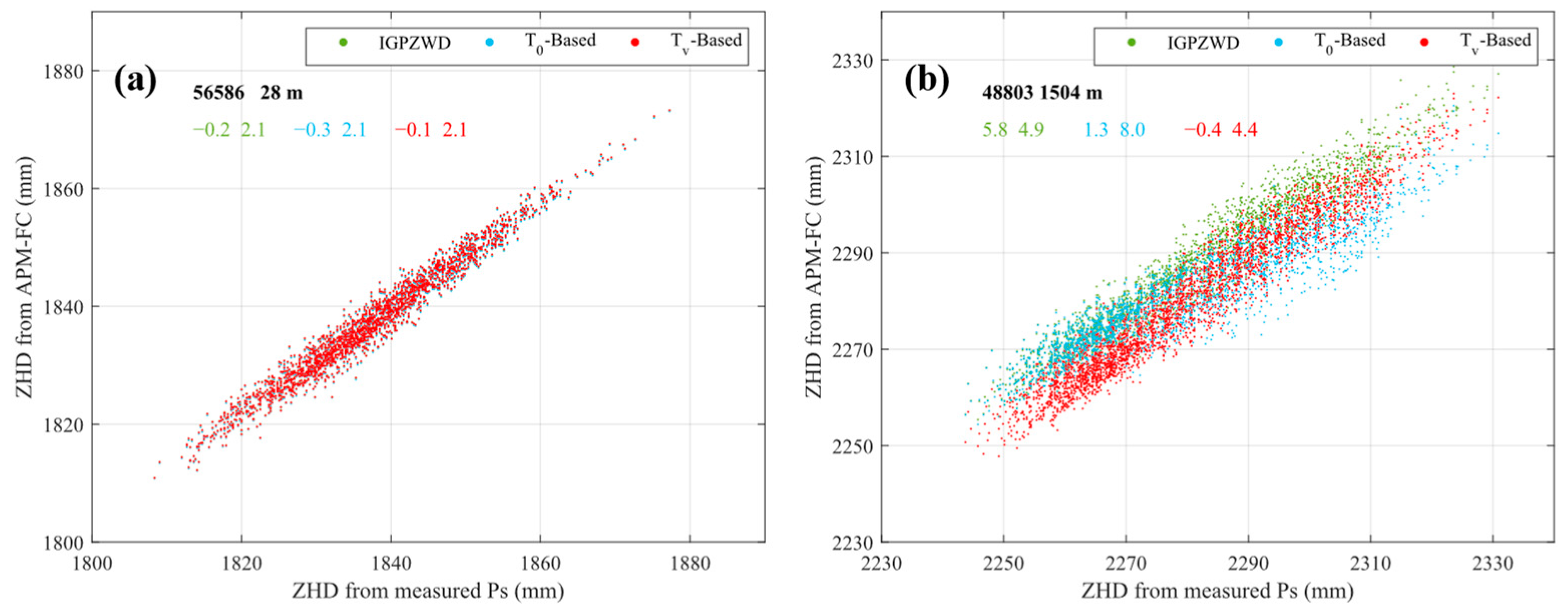
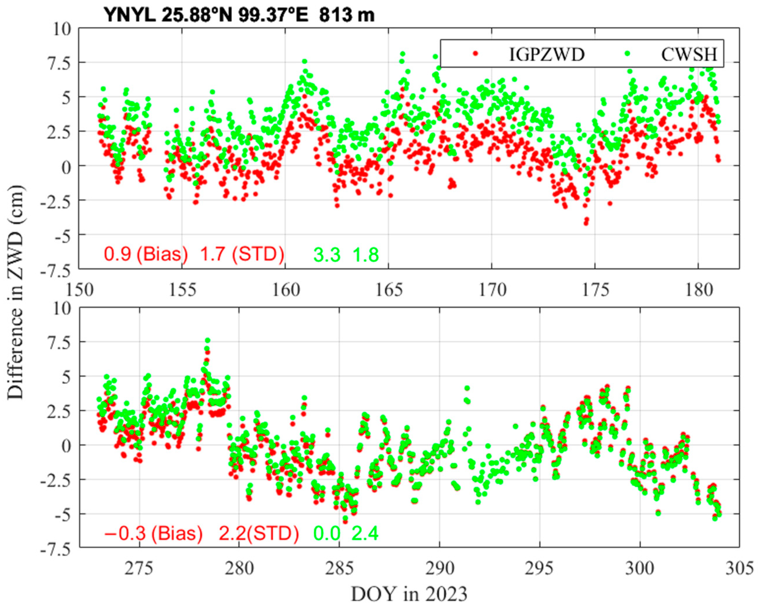
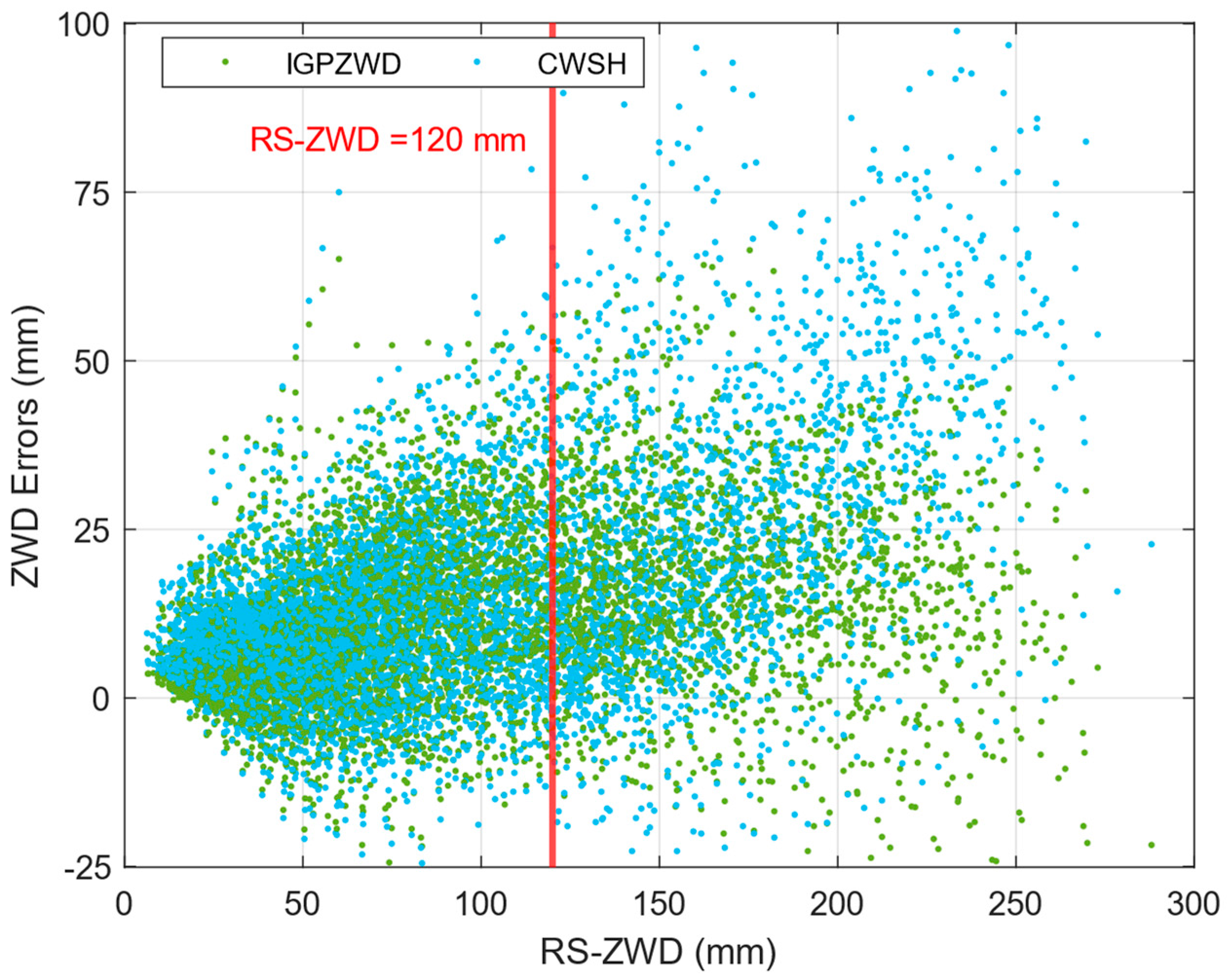
3.2. The Vertical Reduction Models Validated by Measured Meteorological Data
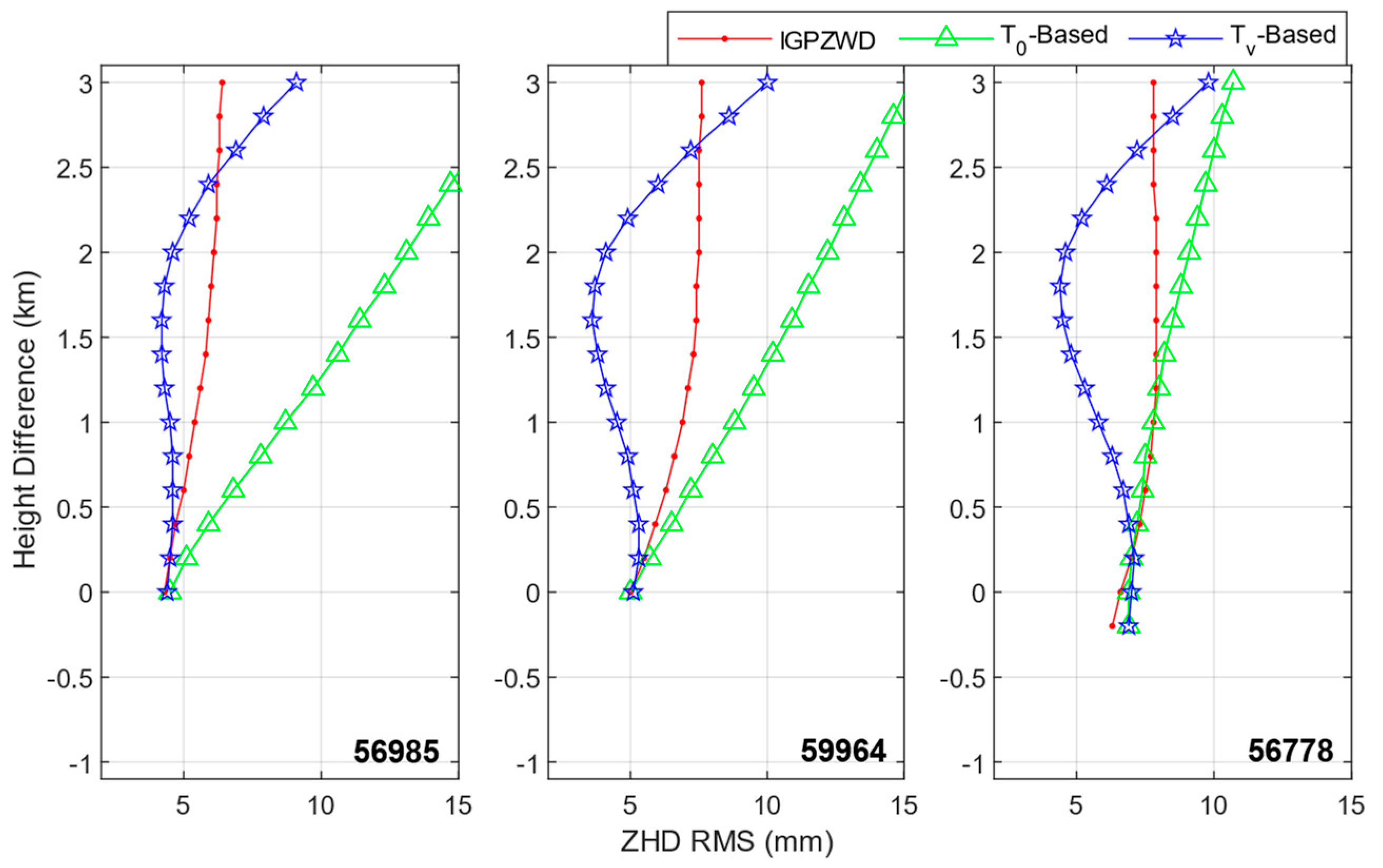
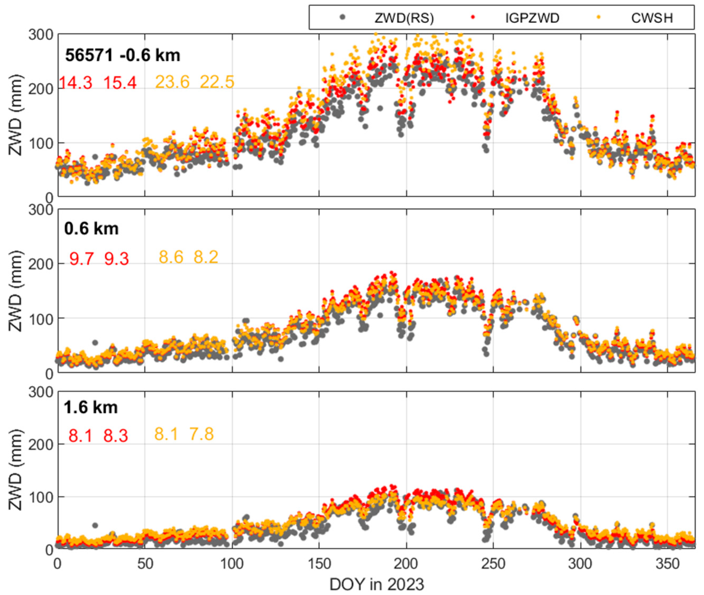
3.3. The Vertical Reduction Models Validated by Radiosondes
4. Conclusions
Author Contributions
Funding
Institutional Review Board Statement
Informed Consent Statement
Data Availability Statement
Acknowledgments
Conflicts of Interest
References
- Böhm, J.; Schuh, H. Atmospheric Effects in Space Geodesy; Springer: Berlin/Heidelberg, Germany, 2013; Volume 5. [Google Scholar]
- Lu, C.; Zhong, Y.; Wu, Z.; Zheng, Y.; Wang, Q. A tropospheric delay model to integrate ERA5 and GNSS reference network for mountainous areas: Application to precise point positioning. GPS Solut. 2023, 27, 81. [Google Scholar] [CrossRef]
- Bevis, M.; Businger, S.; Herring, T.A.; Rocken, C.; Anthes, R.A.; Ware, R.H. GPS meteorology: Remote sensing of atmospheric water vapor using the global positioning system. J. Geophys. Res. Atmos. 1992, 97, 15787–15801. [Google Scholar] [CrossRef]
- Davis, J.; Herring, T.; Shapiro, I.; Rogers, A.; Elgered, G. Geodesy by radio interferometry: Effects of atmospheric modeling errors on estimates of baseline length. Radio Sci. 1985, 20, 1593–1607. [Google Scholar] [CrossRef]
- Hopfield, H.S. Tropospheric effect on electromagnetically measured range: Prediction from surface weather data. Radio Sci. 1971, 6, 357–367. [Google Scholar] [CrossRef]
- Saastamoinen, J. Atmospheric correction for the troposphere and stratosphere in radio ranging of satellites. In Proceedings of the 3rd International Symposium on the Use of Artificial Satellites for Geodesy, Washington, DC, USA, 15–17 April 1971; pp. 247–251. [Google Scholar]
- Böhm, J.; Möller, G.; Schindelegger, M.; Pain, G.; Weber, R. Development of an improved empirical model for slant delays in the troposphere (GPT2w). GPS Solut. 2015, 19, 433–441. [Google Scholar] [CrossRef]
- Lagler, K.; Schindelegger, M.; Böhm, J.; Krásná, H.; Nilsson, T. GPT2: Empirical slant delay model for radio space geodetic techniques. Geophys. Res. Lett. 2013, 40, 1069–1073. [Google Scholar] [CrossRef]
- Landskron, D.; Böhm, J. VMF3/GPT3: Refined discrete and empirical troposphere mapping functions. J. Geod. 2018, 92, 349–360. [Google Scholar] [CrossRef]
- Zhang, H.; Yuan, Y.; Li, W. Real-time wide-area precise tropospheric corrections (WAPTCs) jointly using GNSS and NWP forecasts for China. J. Geod. 2022, 96, 44. [Google Scholar] [CrossRef]
- Zhou, Y.Z.; Lou, Y.D.; Zhang, W.X.; Kuang, C.L.; Liu, W.X.; Bai, J.N. Improved performance of ERA5 in global tropospheric delay retrieval. J. Geod. 2020, 94, 103. [Google Scholar] [CrossRef]
- Dousa, J.; Elias, M. An improved model for calculating tropospheric wet delay. Geophys. Res. Lett. 2014, 41, 4389–4397. [Google Scholar] [CrossRef]
- Wang, J.; Balidakis, K.; Zus, F.; Chang, X.; Ge, M.; Heinkelmann, R.; Schuh, H. Improving the Vertical Modeling of Tropospheric Delay. Geophys. Res. Lett. 2022, 49, e2021GL096732. [Google Scholar] [CrossRef]
- Berberan-Santos, M.N.; Bodunov, E.N.; Pogliani, L. On the barometric formula. Am. J. Phys. 1997, 65, 404–412. [Google Scholar] [CrossRef]
- Askne, J.; Nordius, H. Estimation of tropospheric delay for microwaves from surface weather data. Radio Sci. 1987, 22, 379–386. [Google Scholar] [CrossRef]
- Hobiger, T.; Ichikawa, R.; Koyama, Y.; Kondo, T. Fast and accurate ray-tracing algorithms for real-time space geodetic applications using numerical weather models. J. Geophys. Res. Atmos. 2008, 113, D20302. [Google Scholar] [CrossRef]
- Böhm, J.; Schuh, H. Forecasting Data of the Troposphere Used for IVS Intensive Sessions. In Proceedings of the 18th EVGA Working Meeting & 8th IVS Analysis Workshop, 2nd IVS VLBI2010 Working Meeting, Vienna, Austria, 12–15 April 2007. [Google Scholar]
- Böhm, J.; Kouba, J.; Schuh, H. Forecast Vienna Mapping Functions 1 for real-time analysis of space geodetic observations. J. Geod. 2009, 83, 397–401. [Google Scholar] [CrossRef]
- Yuan, P.; Blewitt, G.; Kreemer, C.; Hammond, W.C.; Argus, D.; Yin, X.; Van Malderen, R.; Mayer, M.; Jiang, W.; Awange, J.; et al. An enhanced integrated water vapour dataset from more than 10,000 global ground-based GPS stations in 2020. Earth Syst. Sci. Data Discuss. 2022, 15, 723–743. [Google Scholar] [CrossRef]
- Chen, B.; Yu, W.; Wang, W.; Zhang, Z.; Dai, W. A global assessment of precipitable water vapor derived from GNSS zenith tropospheric delays with ERA5, NCEP FNL, and NCEP GFS products. Earth Space Sci. 2021, 8, e2021EA001796. [Google Scholar] [CrossRef]
- Zhang, H. Study on BDS/GNSS Tropspheric Modeling under Complex Conditions; The Innovation Academy for Precision Measurement Science and Technology (APM), Chinese Academy of Sciences (CAS): Wuhan, China, 2022. [Google Scholar]
- Zhang, H.; Yuan, Y.; Li, W.; Ji, D.; Lv, M. Implementation of Ready-Made Hydrostatic Delay Products for Timely GPS Precipitable Water Vapor Retrieval Over Complex Topography: A Case Study in the Tibetan Plateau. IEEE J. Sel. Top. Appl. Earth Obs. Remote Sens. 2021, 14, 9462–9474. [Google Scholar] [CrossRef]
- Jiang, C.; Gao, X.; Zhu, H.; Wang, S.; Liu, S.; Chen, S.; Liu, G. An improved global pressure and ZWD model with optimized vertical correction considering the spatial-temporal variability of multiple height scale factors. EGUsphere 2024, 2024, 1–25. [Google Scholar]
- Li, W.; Yuan, Y.; Ou, J.; He, Y. IGGtrop_SH and IGGtrop_rH: Two improved empirical tropospheric delay models based on vertical reduction functions. IEEE Trans. Geosci. Remote Sens. 2018, 56, 5276–5288. [Google Scholar] [CrossRef]
- Yao, Y.; Hu, Y. An empirical zenith wet delay correction model using piecewise height functions. In Annales Geophysicae; Copernicus Publications: Göttingen, Germany, 2018; pp. 1507–1519. [Google Scholar]
- Kleijer, F. Troposphere Modeling and Filtering for Precise GPS Leveling. Ph.D. Thesis, TU Delft Faculty of Aerospace Engineering, Delft, The Netherlands, 2004. [Google Scholar]
- Li, T.; Wang, L.; Chen, R.; Fu, W.; Xu, B.; Jiang, P.; Liu, J.; Zhou, H.; Han, Y. Refining the empirical global pressure and temperature model with the ERA5 reanalysis and radiosonde data. J. Geod. 2021, 95, 31. [Google Scholar] [CrossRef]
- Kouba, J. Implementation and testing of the gridded Vienna Mapping Function 1 (VMF1). J. Geod. 2008, 82, 193–205. [Google Scholar] [CrossRef]
- Li, Q.; Yuan, L.; Jiang, Z. Modeling tropospheric zenith wet delays in the Chinese mainland based on machine learning. Gps Solut. 2023, 27, 171. [Google Scholar] [CrossRef]
- Li, Q.; Böhm, J.; Yuan, L.; Weber, R. Global zenith wet delay modeling with surface meteorological data and machine learning. GPS Solut. 2024, 28, 57. [Google Scholar] [CrossRef]


| Model | Biases Mean [Min, Max] | STD Mean [Min, Max] |
|---|---|---|
| IGPZWD | 1.0 [−3.5, 6.1] | 2.3 [1.5, 5.9] |
| -based model | −0.3 [−7.1, 6.7] | 2.7 [1.5, 8.0] |
| -based model | 0.4 [−3.0, 5.3] | 2.3 [1.4, 4.4] |
| Model | Biases Mean [Min, Max] | STD Mean [Min, Max] |
|---|---|---|
| IGPZWD | 0.4 [−1.4, 1.6] | 1.8 [1.2, 2.8] |
| Constant WSH | 0.7 [2.5, 4.3] | 1.9 [1.2, 3.3] |
Disclaimer/Publisher’s Note: The statements, opinions and data contained in all publications are solely those of the individual author(s) and contributor(s) and not of MDPI and/or the editor(s). MDPI and/or the editor(s) disclaim responsibility for any injury to people or property resulting from any ideas, methods, instructions or products referred to in the content. |
© 2024 by the authors. Licensee MDPI, Basel, Switzerland. This article is an open access article distributed under the terms and conditions of the Creative Commons Attribution (CC BY) license (https://creativecommons.org/licenses/by/4.0/).
Share and Cite
Zhou, F.; Li, L.; Wang, Y.; Dai, Z.; Ding, C.; Li, H.; Yuan, Y. Analysis of Different Height Correction Models for Tropospheric Delay Grid Products over the Yunnan Mountains. Atmosphere 2024, 15, 872. https://doi.org/10.3390/atmos15080872
Zhou F, Li L, Wang Y, Dai Z, Ding C, Li H, Yuan Y. Analysis of Different Height Correction Models for Tropospheric Delay Grid Products over the Yunnan Mountains. Atmosphere. 2024; 15(8):872. https://doi.org/10.3390/atmos15080872
Chicago/Turabian StyleZhou, Fangrong, Luohong Li, Yifan Wang, Zelin Dai, Chenchen Ding, Hui Li, and Yunbin Yuan. 2024. "Analysis of Different Height Correction Models for Tropospheric Delay Grid Products over the Yunnan Mountains" Atmosphere 15, no. 8: 872. https://doi.org/10.3390/atmos15080872