Article

The Historical and Future Variations of Water Conservation in the Three-River Source Region (TRSR) Based on the Soil and Water Assessment Tool Model

1
State Key Laboratory of Earth Surface Processes and Resource Ecology, Faculty of Geographical Science, Beijing Normal University, Beijing 100875, China
2
School of Mathematics and Computational Science, Key Laboratory of Intelligent Control Technology for Wuling-Mountain Ecological Agriculture in Hunan Province, Huaihua University, Huaihua 418008, China
*
Authors to whom correspondence should be addressed.
Atmosphere 2024, 15(8), 889; https://doi.org/10.3390/atmos15080889
Submission received: 30 June 2024 / Revised: 21 July 2024 / Accepted: 22 July 2024 / Published: 25 July 2024
(This article belongs to the Special Issue Observation and Modeling of Evapotranspiration)

Abstract

:
Water conservation is an essential parameter for maintaining the ecological balance. The Three-River Source Region (TRSR) cannot be an exception, since it is one of the most influential water conservation reserves in the Qinghai–Tibet Plateau in China. Therefore, the realization of its scientific significance can determine its future regional sustainable development and the optimal allocation of water resources. The study of the past is critical to predict the future temporal and spatial changes in the water conservation of the TRSR. The first task of this study was to obtain the optimal runoff simulations in the TRSR from 1981 to 2014 by calibrating the adjustable the parameters of the Soil and Water Assessment Tool (SWAT) model. Then, the water conservation of the TRSR from 1981 to 2014 was quantified. Finally, the future water conservation of the TRSR was also predicted using the optimal SWAT model. The predication took into consideration the three terms including the near-term (2015–2044), mid-term (2045–2074), and long-term (2075–2099) in three different climate scenarios of SSP1-1.9 (SSP119), SSP2-4.5 (SSP245), and SSP5-8.5 (SSP585). The main findings are as follows: (1) both the coefficient of determination (R2) and Nash–Sutcliffe efficiency coefficient (NSE) for runoff simulation on the three sub-basins reached above 0.78 during the calibration and validation periods, which indicates the reasonableness of the SWAT model in the TRSR. (2) From 1981 to 2014, the water conservation capacity of the TRSR showed an increasing trend (0.5135 mm/year), and its changes had significant positive correlations with precipitation and temperature. The Yellow River Source (YR) and the Yangtze River Source (YZ) had the strongest and weakest water conservation capacities, respectively. (3) From 2015 to 2099, the water conservation in the TRSR in the SSP119, SSP245, and SSP585 scenarios decreased first and then increased, increased first and then decreased, and increased steadily, respectively.

1. Introduction

The water conservation function is one of the most significant service functions of ecosystems [1]. Water conservation refers to the interception and seepage of precipitation from vegetation canopy, dead leaves, and soil [2], which participate in the water cycle by affecting precipitation, runoff, evapotranspiration, and seepage [3,4]. With the development of the human society, the destruction of water resources by human activities has become increasingly serious, and the depletion and continuous reduction in water resources have forced human beings to pay more attention to it, making the assessment and analysis of the water conservation function a key point of the study of ecological service function [5].
The Three-River Source Region (TRSR), located on the Qinghai–Tibetan Plateau in southwestern China, is the birthplace of the Yangtze River, the Lancangjing River, and the Yellow River. It is not only an important water supply area in China, but also a “water tower” for many countries in Southeast Asia and South Asia, so the study of the water conservation function in the TRSR is of great significance. In addition, it is conducive to the study of the changes in the ecological environment of the region, which has an enormous ecological reference value for the establishment of the ecological security barrier in the Qinghai–Tibetan Plateau in the future.
Currently, there are two popular physical models to estimate water conservation capacity: the Integrated Valuation of Ecosystem Services and Tradeoffs (InVEST) model and the Soil and Water Assessment Tool (SWAT) model. Compared to the InVEST model, the SWAT model can provide a finer resolution of simulation results. For instance, the highest temporal resolution for the SWAT model is daily, while the highest temporal resolution for the InVEST model is monthly. In addition, the SWAT model provides more detailed descriptions on hydrological and eco-physical processes, such as surface runoff, underground runoff, and evapotranspiration. Therefore, the more accurate water conservation capacity can be obtained by the SWAT model rather than the InVEST model.
The SWAT model is a comprehensive hydrologic simulation program developed by USDA Agricultural Research Service (ARS) in the mid-1980s [6]. Since its inception, the SWAT model has been widely used in hydrology-related fields. For instance, in many countries, such as in Africa [7], in Southeast Asia [8,9], in Europe [10,11], and the United States [12], the SWAT model has been widely used for the assessment of climate change, water resource management, and groundwater recharge, etc. In China, many runoff simulations have been conducted by the SWAT model such as in the Jinsha River Basin [13], the Golmud River Basin [14], the Han River Basin [15], and the Minjiang River Basin [16]. In addition to runoff, the simulations of nitrogen and phosphorus surface pollution in agricultural fields [17], sand production [18], and soil moisture [19] have also been conducted by the SWAT model. Since the SWAT model can calculate runoff at monthly or even daily scales, which considerably improves the temporal accuracy of hydrological process simulations compared with previous models, regional water conservation studies based on the SWAT model have begun to appear. For example, Chen et al. [20] used an improved SWAT model to simulate the impacts of agricultural production activities on water conservation and crop yields in the Texas High Plains. Li et al. [21] evaluated the impacts of land use change on water conservation in the Beijing–Tianjin–Hebei region of China. Lin et al. [22] analyzed the spatial and temporal change patterns of forest water conservation in the Jinjiang River Basin of the Southeast Coast in China from 2002 to 2010 based on the SWAT model. Li et al. [23] used the SWAT model to assess the impacts of climate change and land use on changes in the water conservation capacity of the TRSR, but they did not analyze the contribution of meteorological and hydrological drivers to water conservation capacity, nor did they predict the changes in water conservation capacity in different climate scenarios in the future.
Today, climate change is recognized all peoples. The Sixth Assessment Report (AR6) of the Intergovernmental Panel on Climate Change (IPCC), launched from 2021 to 2023, offers five different future climate change scenarios corresponding to the different global warming temperatures [24]. By simulating multiple scenarios, researchers and policymakers can assess the uncertainties and risks associated with different levels of greenhouse gas emissions and potential climate responses. This helps in developing robust adaptation and mitigation strategies to address the challenges posed by climate change on ecosystems, societies, and economies. The AR6 took 2015 as the dividing line to distinguish the past from the future. Therefore, this study selected the past 34 years of 1981–2014 to analyze the variations of the historical water conservation, and the rest 85 years in the 21st century to predict the variations of the future water conservation in the TRSR.
This study aimed to analyze the variations of the historical water conservation and make predictions of the variations of the future water conservation in the TRSR, so as to provide a valuable reference for ecological protection and water resource management in the region. Therefore, this study used the SWAT model to simulate the spatial and temporal changes in water conservation in the TRSR over the past 34 years (1981–2014) and nearly 100 years into the future (2015–2099) in three different scenarios. The structure of the article is organized as follows: the first section introduces the concept and significance of water conservation and some relative studies. The second section briefly introduces the study area, the SWAT model, and the related driving and validation data. The simulation results of historical and future water conservation are presented in the third section. Finally, the discussion and conclusions are presented in the fourth and fifth sections, respectively.

2. Materials and Methods
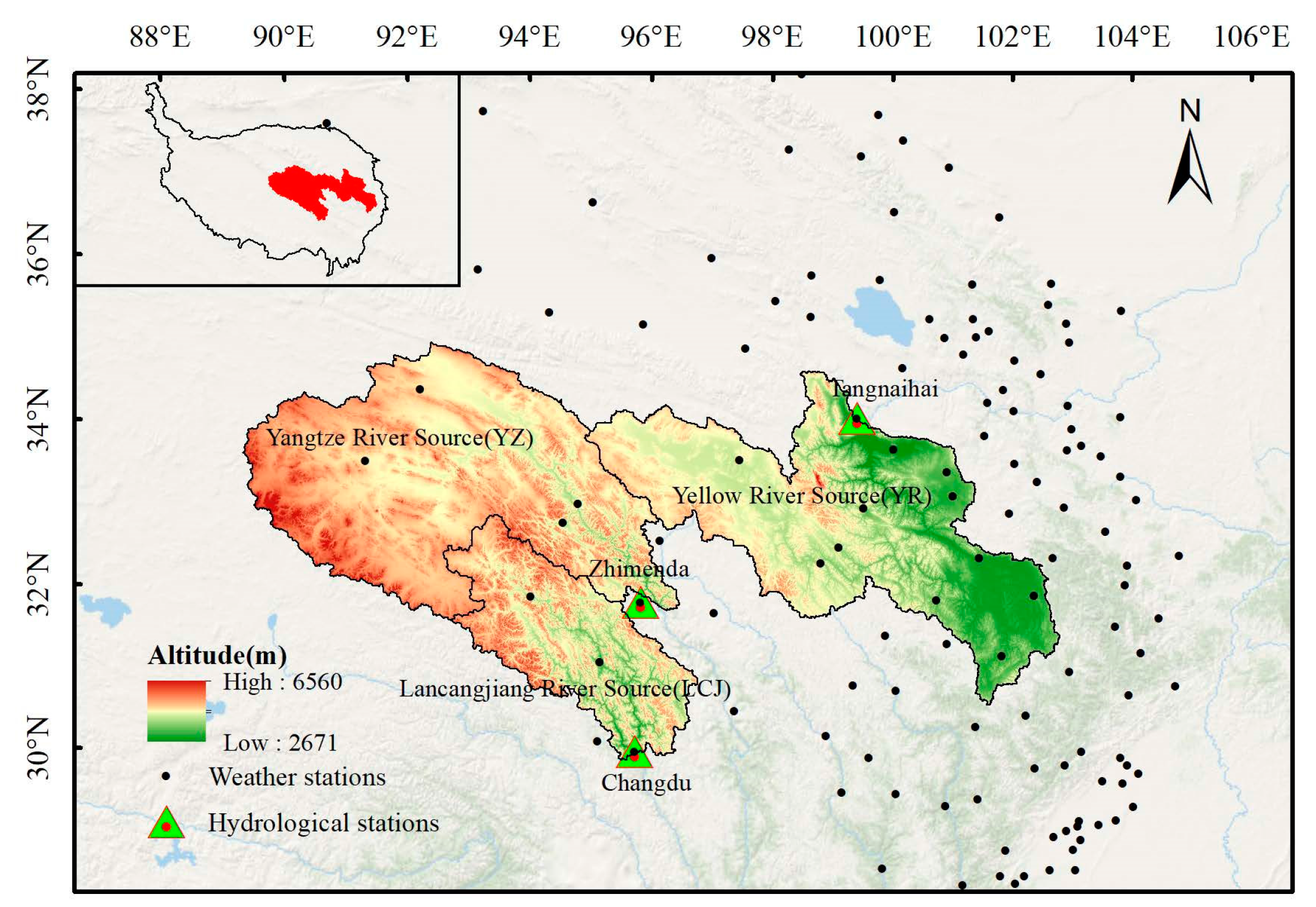
2.1. Region

The study area is located northeast of the Qinghai–Tibet Plateau and south of Qinghai Province. The TRSR includes the Yangtze River source (YZ), Yellow River source (YR), and Lancangjing River source (LCJ). Covering approximately 364,000 square kilometers with an average altitude of over 4000 m, the region features a unique plateau climate and complex geographical environment. The location and elevation of the Three Rivers’ source area are shown in Figure 1.

2.2. Data

The datasets of the digital elevation model (DEM), runoff, land use, soil, meteorology, and river network were used in this study. A brief overview of these datasets is provided as follows.
The DEM data are based on the Shuttle Radar Topography Mission (SRTM) data with a spatial resolution of 90 m obtained by NASA and other institutions through the radar system on the space shuttle in 2000 to provide global elevation data. These data were downloaded from the National Science Data Center (https://data.tpdc.ac.cn/home (accessed on 1 March 2023)) of the Qinghai–Tibet Plateau.
The runoff data include measured data from hydrology stations at the sources of the YR (Tangnaihai), the YZ (Zhimenda), and the LCJ (Changdu) over many years, collected from the China Hydrology Statistical Yearbook. These data were used to calibrate the SWAT model, and the details of the three sites are shown in Table 1.
The land use data were sourced from the Resources and Environmental Sciences and Data Center, Chinese Academy of Sciences, covering the period from 1980 to 2015. The data from 2000 were used as the driving data for the SWAT model and reclassified to the types of grassland, glacier, and snow.
The soil data were obtained from the United Nations Food and Agriculture Organization (FAO) and the Vienna International Institute for Applied Systems Analysis (IIASA) World Harmonized Soil Database (HWSD: https://www.fao.org/home/en/ (accessed on 10 March 2023)), with a resolution of 1 km.
The meteorological data were from the Daily Values of China Surface Climatological Data (V3.0) of the China Meteorological Administration. There are over 2400 meteorological stations in China, and 103 of them in and around the TRSR were selected to run the SWAT model. The meteorological data include precipitation, maximum temperature, minimum temperature, relative humidity, solar radiation, and wind speed. These weather elements were used to create the weather generator for the SWAT model. Note that the deficiency in the meteorological posts in the western part of the TRSR may cause some uncertainties in the hydrological simulations of the region.
To simulate the hydrological process more accurately, the 5th level of the river network presented in the smallest grade watersheds with areas lower than 100 km2 in China was downloaded from the National Catalogue Service for Geographic Information (https://www.webmap.cn/commres.do?method=dataDownload (accessed on 1 May 2023)) and used to generate finer network of waterways for accurate runoff simulations.
The future climate scenario data mainly include daily rainfall and climate data. The CAMS-CSM1-0 model data (https://cmip-publications.llnl.gov/view/CMIP6/?type=model&option=CAMS-CSM1-0 (accessed on 1 July 2023)), developed by the Institute of Atmospheric Physics, Chinese Academy of Sciences, under the framework of CMIP6 (Sixth Global Climate Model Comparison Program), was used in this study. In the CMIP6 project, “Shared Socio-economic Pathways” (SSPs) are a new tool used to describe possible future scenarios of social development and environmental change [24]. This study selected three major SSPs for analysis as follows:
(1)
SSP1-1.9 (SSP119): Sustainable development path
In the SSP119 scenario, the global community moves towards a lower carbon future, with the goal of limiting global temperature rise to 1.5 °C. Model projections show a small increase in global mean temperature over pre-industrial levels and relatively stable changes in precipitation in this scenario. This path is characterized by enhanced climate mitigation measures, including large-scale renewable energy applications and global greening projects, to effectively control the impact of climate change on ecosystems and human habitats.
(2)
SSP2-4.5 (SSP245): Medium development path
The SSP245 scenario assumes moderate global economic growth and climate change mitigation. In this scenario, models predict that global average temperatures could rise by about 2 °C by 2100. Precipitation patterns show increased precipitation over equatorial regions and high latitudes, especially over the Asian monsoon and high latitudes of North America, where more extreme precipitation events likely occur. Some regions in the mid-latitudes, such as the Mediterranean, may experience a decrease in precipitation.
(3)
SSP5-8.5 (SSP585): High economic growth path
In the SSP585 scenario, a rapid global economic growth and lack of effective control of greenhouse gas emissions lead to a possible increase in global average temperatures of more than 4 °C by 2100. In this scenario, precipitation patterns change significantly, especially in tropical and subtropical regions, where significant increases in precipitation are expected, along with an increase in the frequency and intensity of extreme weather events such as heat waves and heavy rain. Droughts can also occur over a wider area, especially inland areas at mid-latitudes.
In this study, precipitation and temperature data at corresponding locations of meteorological stations in the three scenarios were used as meteorological inputs to run the SWAT model for the future runoff simulations.

2.3. SWAT Model

The SWAT model, version 2012, was used to simulation hydrological elements, such as runoff, evapotranspiration, and soil layer permeability. The model simulates the flow within a set hydrological response unit and calculates the circulation and transfer of runoff and water quality at the outlet of the basin. The equation of water balance is as follows:
S w t = S w 0 + i = 1 t R day   Q surf   E T W seep   Q g w
where S w t is the soil water content (unit: mm) for the tth day;   S w 0 is the initial soil water content (unit: mm);   R d a y is precipitation (unit: mm);   Q s u r f is the surface runoff (unit: mm); ET is the evapotranspiration (unit: mm); W s e e p is the soil layer permeability (unit: mm), indicating the part that penetrates the groundwater;   Q g w is groundwater flow (unit: mm); t is time (unit: day).
The SWAT model divides the sub-watersheds into multiple hydrologic response units (HRUs) and performs hydrological simulations on the HRUs. The water conservation capacity based on the SWAT model can be expressed as follows [23]:
W = P R E E T S U R Q
where W represents the water conservation amount of the entire basin, PRE is the precipitation in the basin, ET represents evapotranspiration, and SURQ represents surface runoff. All of these are measured in millimeters (mm).
The calculation of actual ET was conducted by the SWAT model. According to the input atmospheric datasets, one of three potential ET methods including the Penman–Monteith method [25], Priestiley–Taylor method [26], and Hargreaves method [27] was selected to calculate the potential ET. For instance, The Penman–Monteith method requires solar radiation, air temperature, relative humidity, and wind speed. The Priestley–Taylor method requires solar radiation, air temperature, and relative humidity. The Hargreaves method requires air temperature only. Once total potential ET is determined, the actual evaporation can be calculated. SWAT first calculates evaporation from rainfall intercepted by the plant canopy and then estimates plant transpiration and soil evaporation.
Water conservation coefficient is the ratio of water conservation to precipitation, which can be used to assess how much precipitation is conserved in a region [6]. The larger the water conservation coefficient is, the less water is lost through evapotranspiration and runoff; on the contrary, the more water is lost through evapotranspiration and runoff. The calculation formula for water conservation coefficient is shown as follows:
W i = W P R E
where W i is the water conservation coefficient, W is the water conservation amount, and PRE is the precipitation in the basin.

2.4. Calibration Method

Since the underlying surface conditions and climate driving data in each region are different, the parameters in the model may have different values in different regions. Parameter calibration can help in obtaining more accurate simulation results in a certain region. SWAT-CUP is a built-in parameter calibration tool for SWAT. It supports a variety of calibration algorithms, including Sequential Uncertainty Fitting (SUFI2), Parameter Solution (ParaSol), Particle Swarm Optimization (Particle Swarm Optimization) (PSO), Generalized Likelihood Uncertainty Estimation (GLUE), and MCMC (Markov Chain Monte Carlo) [28,29]. In this study, the SUFI2 algorithm was used for optimization, which is briefly introduced as follows: the SUFI2 algorithm starts by setting the prior range of parameters and then uses an iterative process to refine the parameter space to reduce the uncertainty while maintaining a good match between model output and observation data. The Nash–Sutcliffe efficiency coefficient (NSE) is a commonly used objective function for evaluating the difference between model runoff performance and observations. Finally, SUFI2 uses p-factor and r-factor to evaluate the accuracy and uncertainty range of the model prediction, respectively. Finally, the optimal runoff simulations and the optimal parameters of the SWAT model are realized.

2.5. Evaluation Indicator

The core of the SWAT hydrological simulation is runoff simulation. Through a comparative analysis of simulated flow and measured flow, the model simulation can be evaluated. Here, the NSE [30] is used as the objective function of optimization. In addition, the correlation coefficient (R2) is also used to evaluate the runoff simulation. The evaluation indicators are described as follows:
N S E = 1 i = 1 n ( Q o b s , i Q s i m , i ) 2 i = 1 n ( Q o b s , i Q ¯ o b s ) 2
R 2 = i = 1 n ( Q o b s , i Q ¯ o b s ) ( Q s i m , i Q ¯ s i m ) i = 1 n ( Q o b s , i Q ¯ o b s ) 2 i = 1 n ( Q s i m , i Q ¯ s i m ) 2
S o b s , i is the observation for ith month, Q s i m , i is the simulated value of the ith month, Q ¯ obs is the average of the observations, Q ¯ sim is the average of the simulation, and n is the total number of observations. The range of NSE values is from negative infinity to 1. NSE = 1 indicates that the simulation results of the model perfectly match the observed data; NSE = 0 indicates that the results of the model are as good as the average of the observed data; NSE < 0 indicates that the model results are worse than the average of the observed data. The range of R 2 is [1], and the closer it is to 1, the closer the simulation results are to the measured results.

3. Results

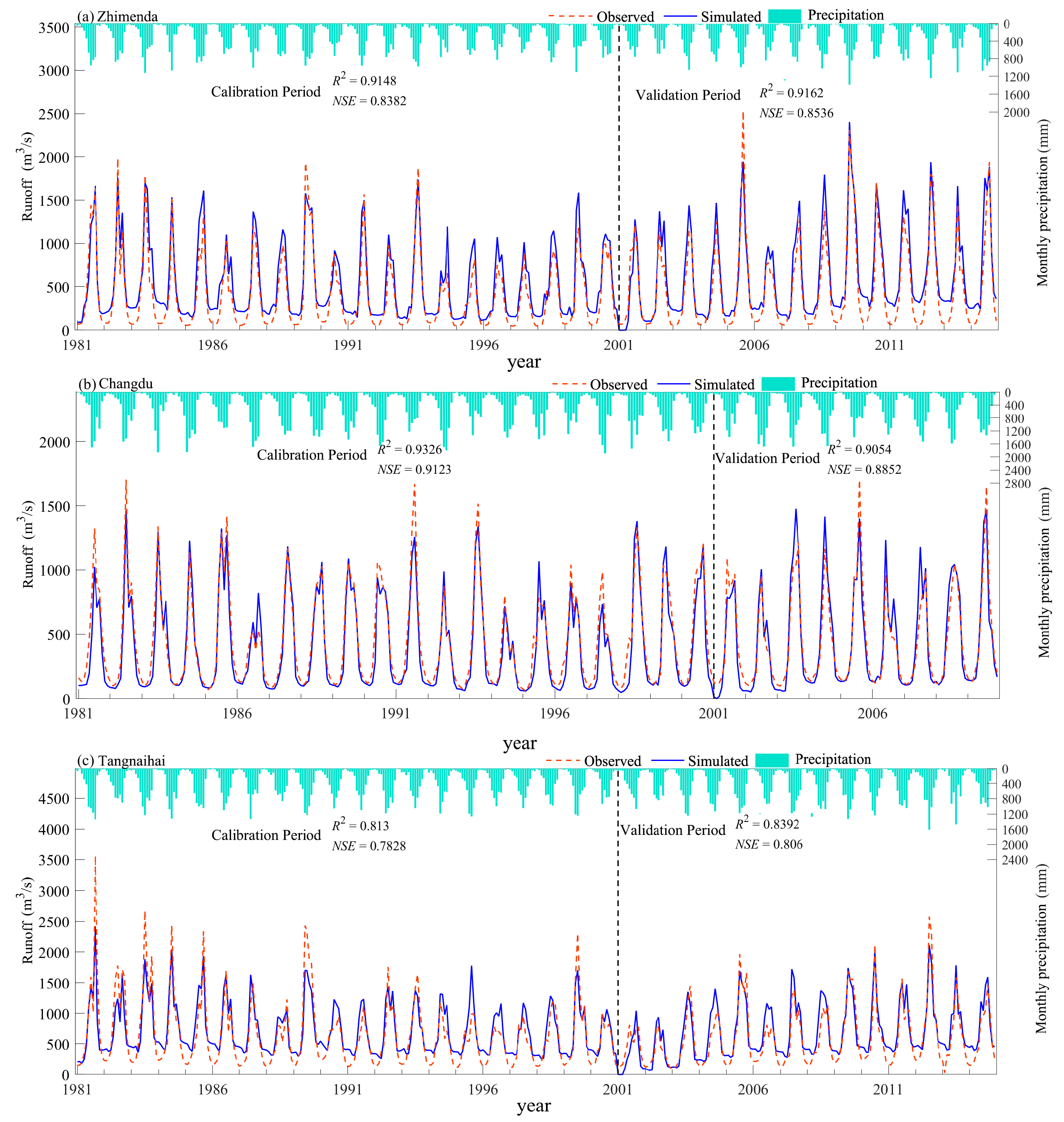
3.1. Model Optimization and Validation

In this study, SWAT-CUP was used to optimize the runoff simulation in the TRSR for obtaining results that are closer to the observed runoff. According to the collected runoff observation data, the calibration periods of three subbasins of TRSR (i.e., YR, YZ, and LCJ) are consistent from 1981 to 2001, while their validation periods are different. The validation periods of the YR and the YZ are 18 years from 2002 to 2019, while the validation period of the LCJ is 8 years from 2002 to 2009. Based on SWAT-CUP, the calibration and validation results of the TRSR runoff are shown in Figure 2. It is found that the simulation result of the LCJ is the best, followed by the YZ and the YR. The simulation of the YR is relatively poor, but the NSE for both the calibration and validation periods is still above 0.78, and the R2 is above 0.8. Note that the NSE of the LCJ for both the calibration and validation periods is over 0.88, and the R2 is over 0.9. Obviously, the simulated runoff in the TRSR is not only consistent with the observation, but the peak of the simulated runoff is also highly consistent with the peak of precipitation. This shows that after calibration and verification, the SWAT model has good applicability in the TRSR.

3.2. Spatiotemporal Variations of Water Conservation in the Three Regions(YR, YZ, and LCJ) from 1981 to 2014

In order to better match the historical scenario simulation of CMIP6, the simulation period for the water conservation of the TRSR was selected as 1981 to 2014. The water conservation was calculated using Formula (2), where the runoff was the optimal runoff simulation results, the evapotranspiration was from the evapotranspiration simulation results obtained by the optimal SWAT simulation, and the precipitation was obtained by interpolation from the station observation.

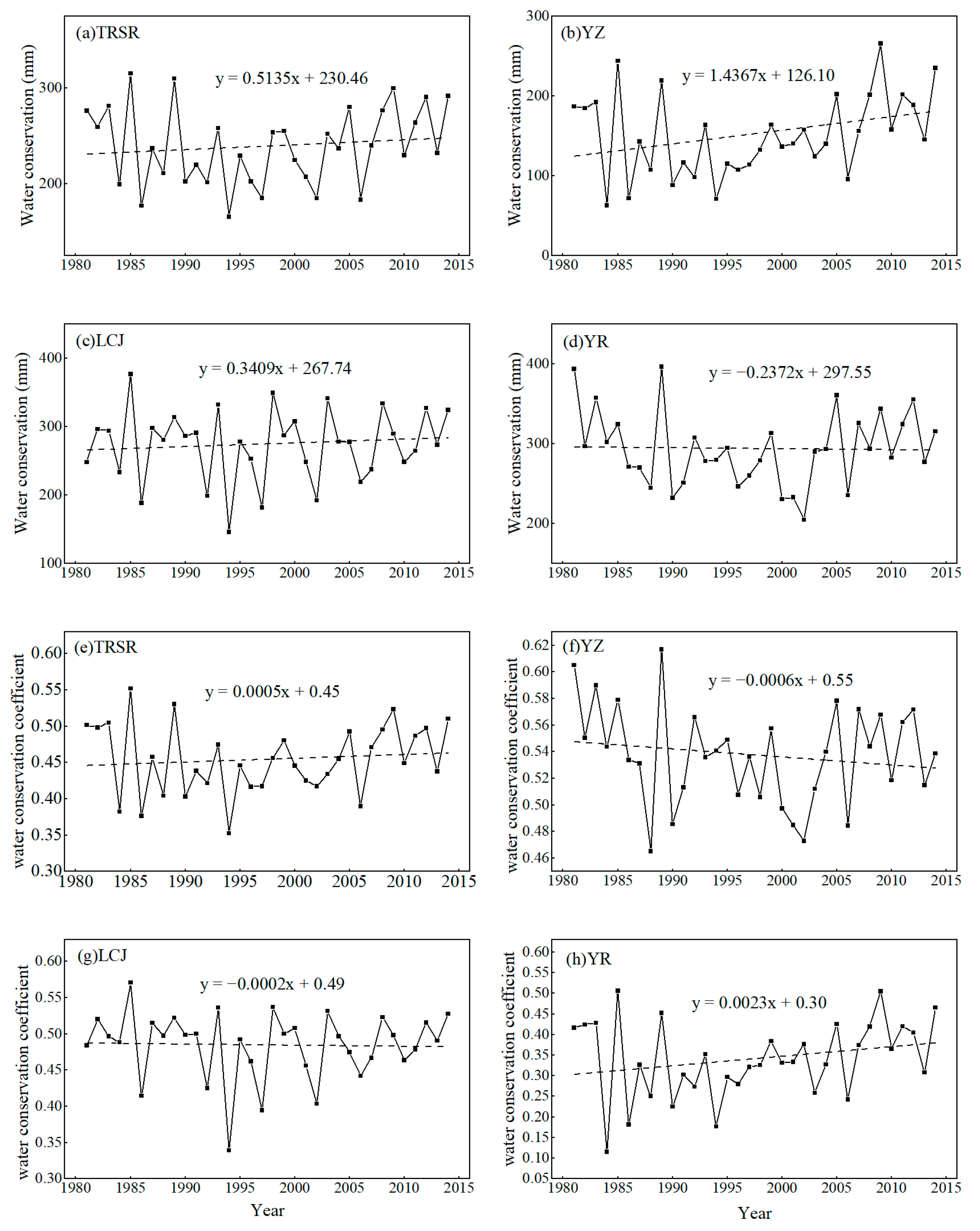
3.2.1. Temporal Variation

Figure 3 shows the annual variation of water conservation capacity and water conservation coefficient in the TRSR and its three sub-basins (YZ, YR, and LCJ). Overall, the water conservation capacity of the TRSR shows an upward trend from 1990 to 2014, with a slope of 0.5135 mm/year. Specifically, the annual water conservation capacity of the YR and LCJ fluctuated around 300 mm, while the annual water conservation of the YZ was less than 300 mm. Therefore, the water conservation of the YR and LCJ was higher than that of the YR. The water conservation of the YZ and LCJ showed an upward trend, with slopes of 1.4367 and 0.3409 mm/year, respectively, while the water conservation of the YR showed a downward trend, with a slope of −0.2372 mm/year.
The water conservation coefficient can reflect the effective interception capacity of the surface to precipitation. Figure 3e–h shows the interannual variation of the water conservation coefficient of the TRSR and its three sub-basins. The water conservation coefficient of the YZ was the highest among the three regions, fluctuating between 0.46 and 0.6, while that of the YR was the lowest, fluctuating below 0.46 in most years, and the water conservation coefficient of the LCJ was between 0.4 and 0.55, which is an intermediate level. The water conservation coefficients of the YZ and the LCJ showed overall downward trends, with the slopes of −0.0006/year and −0.0002/year, respectively; the water conservation coefficient of the YR showed an increasing trend, with the slope of the fitting curve being 0.0023. It is noted that the overall water conservation capacity and water conservation coefficient of the TRSR were both increasing, while for the three sub-regions, the trends of water conservation capacity and water conservation coefficient were opposite.

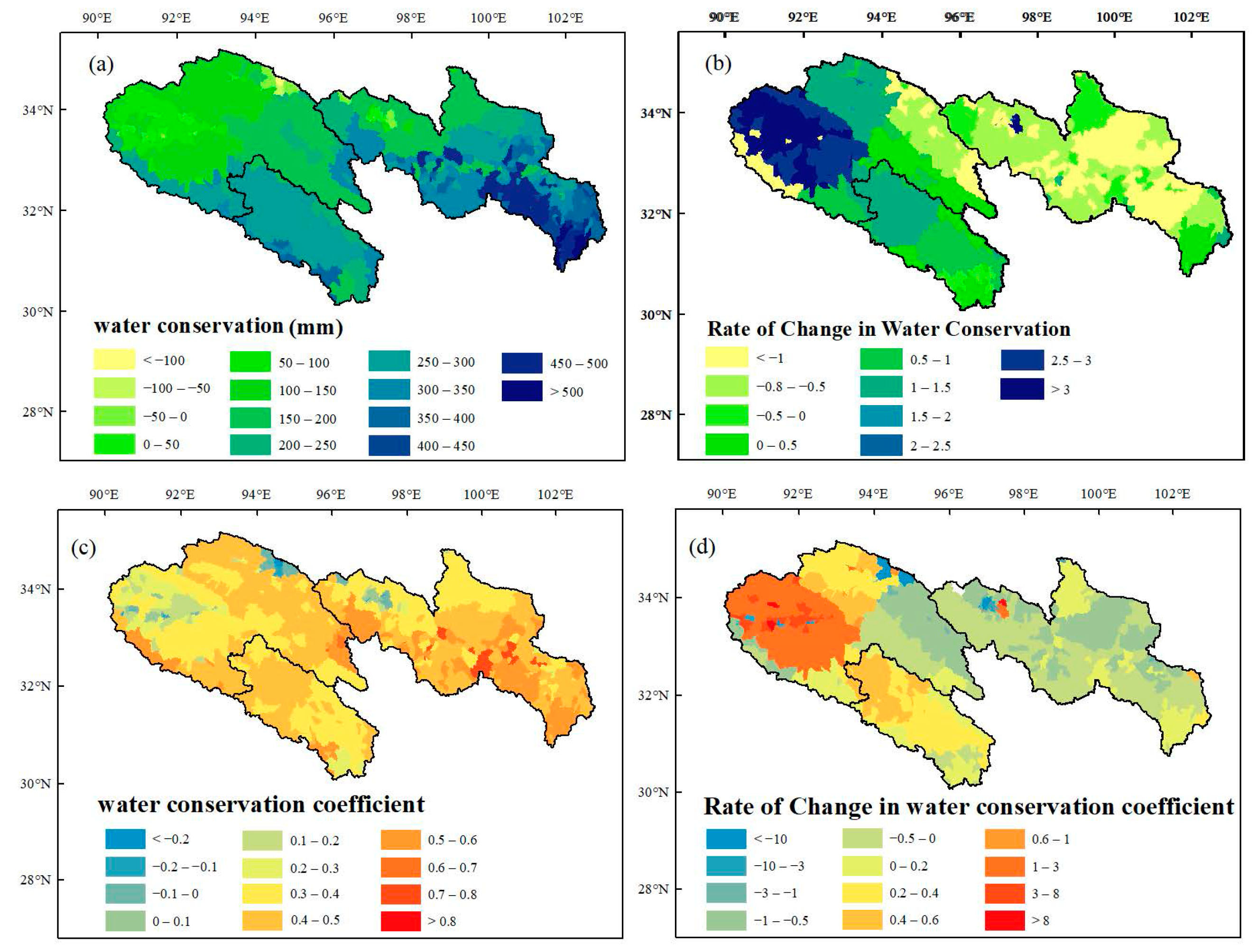
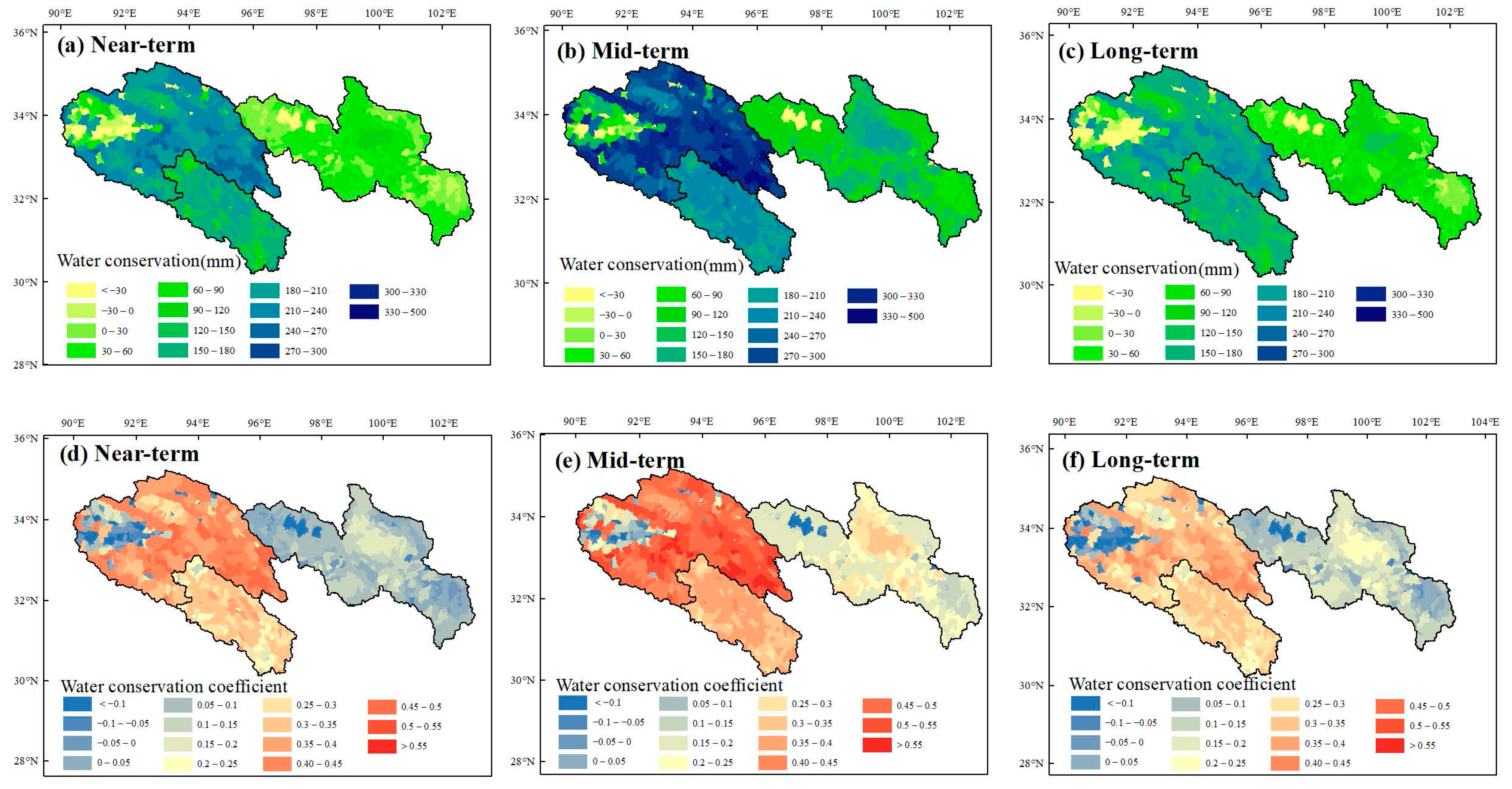
3.2.2. Spatial Variation

The spatial distribution and variations of water conservation capacity in the TRSR from 1981 to 2014 are shown in Figure 4a,b. It can be seen that the area with the largest water conservation was in the southeastern part of the YR, where the annual average water conservation capacity reached more than 400 mm; however, the growth rate of water conservation capacity in this area was not high. This shows that the annual water conservation capacity in the southeastern part of the YR was relatively large, and the change was small. The water conservation capacity in the western part of the YZ was relatively small, but the annual average change rate was relatively high with above 2.5 mm/year, indicating that the water conservation in this area increased significantly. The annual average water conservation capacities in the LCJ were between 50 and 400 mm, which are lower than those in the YR but higher than those in the YZ, and the interannual change was relatively stable, with values basically between 0 and 1.5 mm/year.
The spatial distribution and variations of the water conservation coefficient in the TRSR from 1981 to 2014 are shown in Figure 4c,d. It can be seen that the average water conservation coefficients for more than 90% of the areas in the TRSR from 1981 to 2014 were above 0.3. The high-value area was located in the southeast of the YR, and some of its areas exceed 0.8. The water conservation coefficients in some areas such as the northeast of the YZ and the northwest of the YR were negative. For the areas in the western part of the YZ with a high rate of change in water conservation, the growth rate of the water conservation coefficient was also at a relatively high level (greater than 1) in the TRSR. In other words, the water conservation potential of this area has increased significantly in the past 34 years. Both the water conservation coefficient and its growth rate in the regions with two lakes, Zhaling Lake and Eling Lake in the YR, are relatively low.

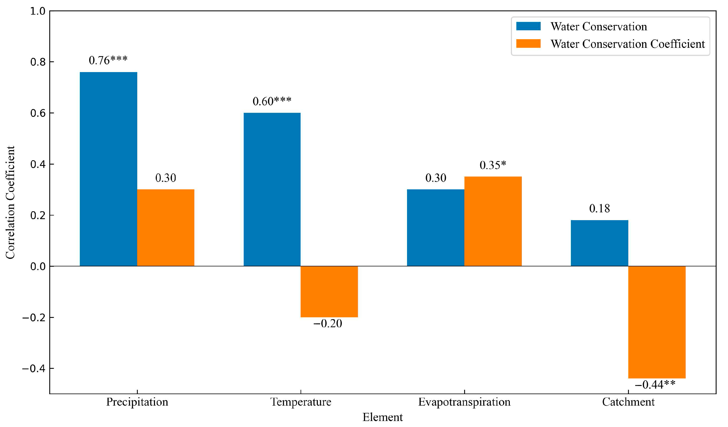
3.2.3. Correlation Analysis between Meteorological and Hydrological Elements and Water Conservation

In order to explore the correlation between the main meteorological and hydrological elements and water conservation, correlation analyses were conducted. Specifically, the correlation coefficients between the meteorological elements (precipitation and temperature) and the water conservation index (water conservation and water conservation coefficient) were calculated. In addition, the correlation coefficients between the hydrological elements (evapotranspiration and catchment amount) and the water conservation index (water conservation and water conservation coefficient) were also calculated. The corresponding results are shown in Figure 5.
As shown in Figure 5, there is a significant positive correlation between precipitation and water conservation capacity, with a correlation coefficient of 0.76, passing the significance test of p < 0.001. It shows that the increase in precipitation significantly increased the water conservation capacity in the TRSR. Precipitation, as the main source of water resources, directly affects the process of water conservation. At the same time, there is also a positive correlation between precipitation and water conservation coefficient, with a correlation coefficient of 0.30. Unfortunately, this result did not pass the significance test of p < 0.05.
The correlation coefficient between temperature and water conservation capacity was 0.60, passing the significance test of p < 0.001. It shows that there is a moderately strong positive correlation with temperature compared with precipitation. This also shows that the increase in temperature may promote the process of water conservation capacity. However, the correlation coefficient between temperature and water conservation coefficient is −0.20 (p > 0.05), indicating that the increase in temperature may reduce the efficiency of water conservation.
The correlation coefficient between evapotranspiration and water conservation capacity is 0.30 (p > 0.05), indicating a weak positive correlation tween the two. It is worth noting that evapotranspiration, as an important link in the water cycle, has a more complex effect on water conservation. The correlation coefficient between evapotranspiration and water conservation coefficient is 0.35, passing the significance test of p < 0.05. It shows that evapotranspiration can promote improvement in the water conservation coefficient.
The correlation coefficient between catchment and water conservation capacity was 0.18 (p > 0.05), showing a weak positive correlation tween the two. Obviously, the increase in the catchment amount does not significantly improve the water conservation capacity, which may also be affected by runoff. However, the correlation between catchment and water conservation coefficient is −0.44 (p < 0.01), indicating that there is a strong negative correlation between the two. The increase in catchment amount will reduce the water conservation coefficient and inhibit the increase in water conservation capacity.

3.3. Temporal and Spatial Changes in Water Conservation in TRSR in the Future

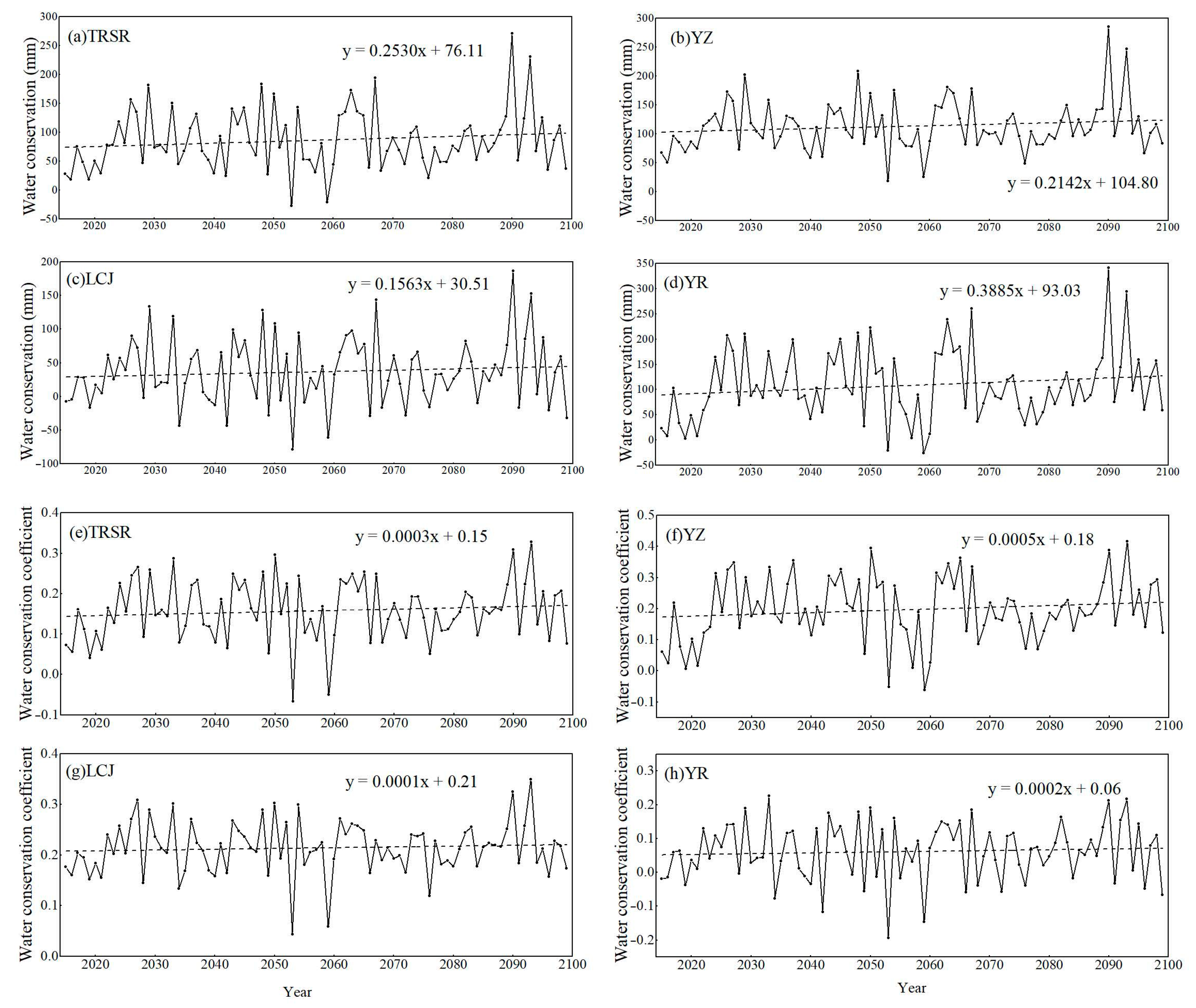
3.3.1. SSP1-1.9 (SSP119) Scenario

The temporal changes in water conservation capacity and water conservation coefficient in the TRSR from 2015 to 2099 in the SSP119 low-emission scenario are shown in Figure 6. It can be seen that both water conservation capacity and water conservation coefficient tend to increase in the future scenario from 2015 to 2100.
The future is divided into three different periods: the near-term of 2015–2044; the mid-term of 2045–2074; and the long-term of 2075–2099. The growth rates of water conservation capacity and water conservation coefficients in TRSR and its three sub-regions in the SSP119 scenario were calculated separately, and the results are shown in Table 2. Overall, the water conservation capacity of the TRSR showed a large inter-annual fluctuation in the near-term, and the slope of the trend line was positive (1.4091 mm/year). However, the fluctuation of the water content coefficient was small, with a trend line slope of 0.0024/year. The trend line slope of water conservation capacity changed to −0.1089 mm/year. In the mid-term, the fluctuation of water conservation coefficient increased slightly, and the slope of the trend line remained at a low level (−0.0002/year), that is, the overall water conservation potential of the TRSR declined.
The fluctuation of the water conservation capacity increased in the long-term, and the slope of the trend line was 2.2681 mm/year, meaning the water conservation capacity of the TRSR in the long-term in the SSP119 scenario increased significantly. The slope of the trend line of the water conservation coefficient recovered to be comparable with that of the near-term (0.0025/year), and the inter-annual fluctuation was relatively stable.
Figure 7 shows the spatial distribution of the water conservation capacity and water conservation coefficient of the TRSR in three different periods in the SSP119 scenario. In the central area, the annual conservation capacity was generally between 100 and 350 mm, indicating that these areas had significant water conservation potential. A similar trend in the overall distribution of water conservation capacity in the mid-term was also observed, but the value of the central high-conservation region was reduced, while that in the western low-conservation region was expanded, suggesting a probable decline in the water conservation capacity of these regions. In the long-term, the high-conservation regions were further concentrated, especially in the middle to the northwestern regions of the YZ, where the water conservation capacity reached above 400 mm in most areas, whereas the water conservation capacity in the east was still weak.
The water conservation coefficient of TRSR in the near-term (Figure 7d) showed significant spatial differences. During this period, the water conservation coefficients of the YR and the western YZ were lower, while those of the southern YZ and the northern LCJ had higher coefficients, accounting for roughly 50% of the total area of the TRSR. In the mid-term (Figure 7e), it can be observed that the high-value region of the water coefficient changed significantly. Basically, the whole TRSR had a water conservation coefficient below 0.25, which was small, showing a significant decrease in the water conservation potential of the TRSR compared with the near-term. Figure 7f displays the spatial distribution of the water conservation coefficient in the long-term of the TRSR. The water conservation coefficients of the YZ and the LCJ were greatly improved, while the water conservation coefficient of the YR was also increased to different degrees. The water conservation coefficient of the YZ was the highest and basically above 0.4. The water conservation coefficient of the LCJ was basically between 0.3 and 0.4, while the water conservation coefficient of the YR was the smallest and basically below 0.3.

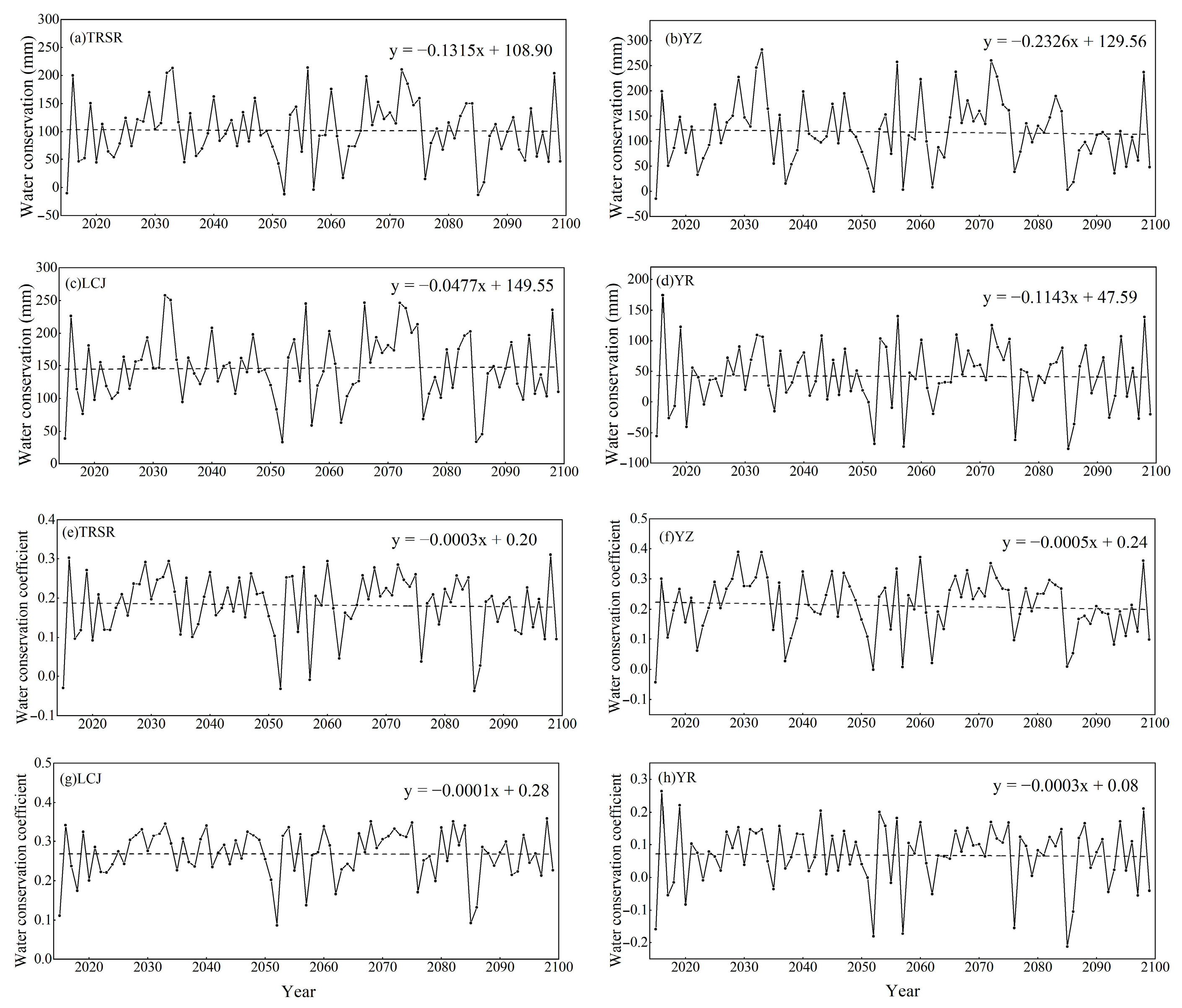
3.3.2. SSP2-4.5 (SSP245) Scenario

SSP245 is a medium-emission scenario, which simulates current emissions without restraint or expansion. Figure 8 shows the temporal changes in water conservation capacity and water conservation coefficients in the TRSR in the medium-emission scenario of SSP245. Generally, the water conservation capacity and water conservation coefficient in the TRSR and its three sub-regions show a downward trend. For the SSP245 scenario, the growth slopes of the water conservation capacity and water conservation coefficient in different periods are shown in Table 3. In the near-term, the TRSR and its three sub-regions exhibit an upward trend, among which the LCJ has the highest upward trend (1.1682 mm/year), and the YR has the smallest upward trend (0.7764 mm/year).
The upward trend of the water conservation capacity in the mid-term continues to accelerate, and the increase rate is about twice that of the near-term. The fastest increase occurs in the YZ (2.7391 mm/year), and the slowest increase occurs in the YR (1.5293 mm/year). In addition, the water conservation coefficient also shows an increasing trend to varying degrees during this period. In the long-term, both the water conservation capacity and water conservation coefficient of the TRSR show a downward trend. The decrease rate of the water conservation capacity in the YZ reach −2.7437 mm/year.
Figure 9 shows the spatial distribution of the water conservation capacity and the water conservation coefficient of the TRSR in three different periods in the SSP245 scenario. Overall, in the SSP245 scenario, the spatial distribution of the water conservation capacity shows obvious spatial heterogeneity, that is, the YZ and the LCJ are generally high, while the YR is generally low. Specifically, in the near-term (Figure 9a), the lowest annual water conservation is mainly concentrated in the YR, with an overall value lower than 90 mm. The annual water conservation capacity of the LCJ is between 100 and 200 mm. Except for the western region, most of the YZ have more than 300 mm, which indicates that the region has a strong water conservation capacity. The regions with the lowest water conservation coefficients of the TRSR in the near-term (index lower than 0.1) are mainly located in the west of the YZ and the northeast of the YR, which is basically consistent with the distribution of the water conservation capacity. The annual water conservation coefficient of most regions of the YZ and the LCJ is higher than 0.2, indicating that the water conservation potential of the YZ and LCJ is higher than that of the YR in this scenario.
Compared with the near-term, the water conservation capacity of the whole TRSR increases significantly in the mid-term (Figure 9b). Among them, the annual water conservation capacity of more than 70% of the YZ reaches more than 270 mm, but the west of the YZ is still a low-value area. The growth of the LCJ is obviously larger than that of the YR, but not as large as that of the YZ. The spatial change trend of the water conservation coefficient in the mid-term is the same as that of the water conservation capacity, that is, the overall water conservation coefficient of the TRSR increases, and the water conservation capacity of the YZ and the LCJ is stronger than that of the YR. The water conservation capacities in Zhaling Lake and Eling Lake in YR and the west of YZ are still low. In the long-term, the overall water conservation capacity declines, and the value of each region falls back to the initial level. The overall water conservation coefficient decreases, and YZ particularly decreases significantly.
By analyzing the spatial distribution and temporal changes in the water conservation capacity and its coefficients in the SSP245 scenario, it can be found that the water conservation and water conservation coefficients of the TRSR show a trend of first increasing and then decreasing in the SSP245 scenario, that is, they are low in the near-term, rise in the mid-term, and then decline again in the long-term. This suggests that in the hypothetical future scenario, the regional water conservation potential might first be improved and then challenged by long-term environmental changes.

3.3.3. SSP5-8.5 (SSP585) Scenarios

The SSP585 scenario posits unbridled human emissions of greenhouse gases. Figure 10 illustrates the temporal fluctuations in water conservation capacity and water conservation coefficient in the SSP585 scenario, spanning the years 2015 to 2099. Broadly speaking, the water conservation capacity and water conservation coefficient of the TRSR and its sub-regions exhibited an upward trend during this timeframe. Table 4 outlines the growth trends of water conservation capacity and conservation coefficients at different intervals in the SSP245 scenario. Overall, the TRSR and its three sub-regions displayed increasing trends across the near-term, mid-term, and long-term. Notably, the initial period saw an overall water conservation capacity growth rate of 0.3165 mm/year in the TRSR, with the fastest growth occurring in the LCJ (0.6318 mm/year) and the slowest in the YR (0.103 mm/year). In the mid-term, there was a significant spike in the growth rate of water conservation capacity across all regions, ranging from 4 to 10 times higher than the preceding period. This period witnessed a rapid increase in water conservation capacity in the TRSR. In the long-term, the growth rate reached its zenith, surpassing that of the earlier stages; particularly notable were the slopes of the YZ and LCJ, exceeding 5 mm/year, and the YR, exceeding 4 mm/year. The growth slope of the water conservation coefficient remained positive throughout all periods, with the long-term’s growth rate being more than three times that of the near-term and mid-term.
Overall, the water conservation capacities of the TRSR and its three sub-regions were manifestly improved from the near-term to long-term. Notably, the LCJ exhibited a notably robust growth rate in water conservation capacity, whereas the water conservation capacity at the YZ experienced a relatively sluggish increase in the near-term and a marked acceleration in the long-term. Furthermore, the water conservation coefficients of the TRSR and its three sub-regions underwent progressive increase from the near-term to the long-term, with a consistent growth rate during the near-term and mid-term, followed by a conspicuous surge in the long-term.
Figure 11 depicts the spatial distribution of water conservation capacity and the water conservation coefficient in three distinct periods in the SSP585 scenario. Overall, the spatial growth trends of water conservation capacity and the conservation coefficient were pronounced in this scenario. Specifically, in the near-term, the water conservation capacity in the TRSR displayed a west-to-east declining trend across the entire area. The LCJ and the southern regions of the YZ exhibited a high annual water conservation capacity, surpassing 120 mm. In contrast, the annual water conservation capacities in the eastern and southern parts of the TRSR were notably lower, falling below 0 mm, indicating a weaker conservation capacity. Areas exhibiting low conservation coefficients, particularly those falling below 0, were predominantly situated at the whole YR and the western edge of the YZ. The conservation coefficient in the central region of the TRSR exceeded 0.1, with the overall weak water conservation capacity in the Tibetan Plateau in this stage in the scenario. In the mid-term, the water conservation capacity at the TRSR notably increased, especially in the LCJ and the YZ, which displayed heightened conservation capacities. Simultaneously, the area with water conservation exceeding 0 mm in the YR appeared to have expanded, albeit retaining insufficient capacity compared to the other two sub-regions during this period. Furthermore, the water conservation coefficients underwent a noteworthy increase in the mid-term, rising from below 0.2 to 0.4 in most areas of the YZ and LCJ, and exceeded −0.1 in the majority of the YR. In the long-term, the high water conservation areas experienced further expansion, markedly escalating the water conservation capacity compared to the preceding period. Most areas in the western and southern parts of the TRSR saw their annual conservation capacity exceed 200 mm, and the YR also achieved a positive conservation level. However, the western part of the YZ and certain parts of the northwest of the YR (Ngoring Lake and Zhaling Lake) remained at relatively low-values. Areas with high values for the water conservation coefficient were also broadened, particularly at the YZ and the LCJ, with water conservation coefficients significantly surpassing those in the mid-term.
Overall, the consistent upward trajectory of water conservation capacity and the water conservation coefficient in the SSP585 scenario underscores the potential of regional ecosystems to adapt to the dynamic variations of climate change and water resources.

4. Discussion

4.1. The Consistency of Runoff Simulaiton with the References

This study utilized the SWAT model to simulate and analyze the spatiotemporal changes in water conservation from the past to the future in the TRSR region. Both R2 and NSE for the calibrated and verified runoff results exceeded 0.78, signifying the high applicability of the SWAT model in the TRSR. Nevertheless, the simulation performance for the YR proved relatively poor, particularly in the simulations of flood peaks and base flows, which may be attributed to the intricate topography and unstable meteorological conditions in the region. Li et al. [31] found that despite the SWAT model demonstrating high applicability in simulating and forecasting runoff in the YR, the simulation accuracy in certain regions remained to be improved due to complex topographic and meteorological conditions. In addition, some studies on past runoff variations occurring in the TRSR are consistent with our study [32,33]. Obviously, these findings are consistent with this study in the TRSR.

4.2. Some Physical Explainations on the Past Water Conservation Changes in the TRSR

The water conservation capacity in the TRSR exhibited a discernible upward trend from 1981 to 2014, with an average increase of 0.5135 mm/year. This trend can be attributed to several factors, such as heightened regional precipitation, temperature, evapotranspiration, and water catchment per unit area [23]. Notably, the water conservation capacity of the YZ and the LCJ experienced annual growth slopes of 1.4367 mm/year and 0.3409 mm/year, respectively. These findings indicate that despite the different variations in precipitation and runoff patterns across the regions, water conservation capacity overall demonstrated a consistent growth over the past few decades. In contrast, the water conservation capacity of the YR displayed a declining trend, with a fitting curve slope of −0.2372 mm/year. This decline is linked to the sluggish increase in precipitation in the YR [23]. Such a phenomenon suggests the existence of notable disparities in the trends of water conservation capacity across different regions under the backdrop of climate change. Further detailed analyses are warranted to elucidate these differences.

4.3. Some Suggestions or Measures to Deal with the Future Water Conservation Changes in Different Emission Scenarios

In the low-emission scenario (SSP119 scenario), the water conservation capacity and the water conservation coefficient in the TRSR exhibit an initial decrease followed by an increase. This implies that global climate mitigation measures in the mid-term are likely to be effective, although their positive impacts may take longer to manifest in local ecosystems. Concurrently, it shows that the water conservation potential of the TRSR region may face certain challenges in the near-term in this scenario. Liu et al. [34] conducted a study on the hydrological processes of the Lhasa River basin in the Tibetan Plateau and found that water conservation capacity may temporarily decline even in the low-emission scenario. Similarly, Zhang et al. [35] found that the same runoff trend occurred in the TRSR from 2010 to 2039. This indicates the reasonability of the obtained water conservation trends in the TRSR. However, as the effectiveness of climate measures extends with time, water conservation capacity is expected to gradually recover and increase in the mid-term and long-term. Obviously, keeping the low-emission scenario will be conducive to water conservation protection.
In the medium-emission scenario (SSP245 scenario), the water conservation capacity and the water conservation coefficient in the TRSR will experience an initial increase followed by a decrease. This indicates that the current emission scenario is not conducive to the sustainable development of the ecological environment in the TRSR. The pattern of change in this scenario suggests that although some positive changes may be observed in the near-term under the existing climate policies, more stringent climate mitigation measures, such as planting short grasses with low water consumption and reducing the planting of forest plants with high water consumption, are necessary in the mid-term and long-term to ensure the sustainability of regional water resources and the stability of the ecosystem stability.
In the high-emission scenario (SSP585 scenario), the water conservation capacity and the water conservation coefficient in the TRSR continue to increase. This outcome may be attributed to improved local vegetation conditions resulting from the melting of snow and ice caused by rising temperatures [36]. However, high-emission scenarios also mean higher climate risks, including more frequent extreme weather event occurrences and more serve damage to the ecosystem. Therefore, although the enhancement of water conservation in this scenario appears to be beneficial, the potential ecological risks should not be overlooked. Therefore, establishing lakes to store glacial meltwater and reducing runoff to the outside of the Qinghai–Tibet Plateau may be an effective solution to maintain the long-term development of water conservation and protect ecological security. He et al. [37] demonstrated that the melting of ice and snow due to rising temperatures in the SSP5-8.5 scenario leads to increased surface runoff, further temporarily improving water conservation capacity. Nonetheless, it is also highlighted that this scenario may trigger more frequent extreme weather events and more serve ecological risks.

5. Conclusions

This study analyzed the historical simulation and future scenario prediction of the water conservation function including water conservation capacity and water conservation coefficient in the TRSR based on the SWAT model, and the main conclusions are as follows:
(1)
By calibrating and validating the runoff simulation results of the SWAT model in the TRSR, it was found that both the R2 and NSE values of the SWAT model exceeded 0.78 in the calibration period and the validation period, which indicates that the model has good applicability in the TRSR.
(2)
During the period of 1981–2014, the overall water conservation capacity and water conservation coefficient of the TRSR showed upward trends. However, different sub-regions behaved differently. For instance, the water source capacities of the YTZ and LC showed upward trends, while the water source capacity of the YL showed a significant decrease. In terms of spatial distribution, the southeastern part of the YR had the highest water conservation capacity, but its growth rate was not high; it even slightly decreased. The western part of the YZ had the lowest water conservation capacity, but its growth rate was the highest. Moreover, the spatial change trend of the water conservation capacity was basically consistent with that of the water conservation coefficient in the TRSR, indicating that both of them had favorable consistency in the TRSR.
(3)
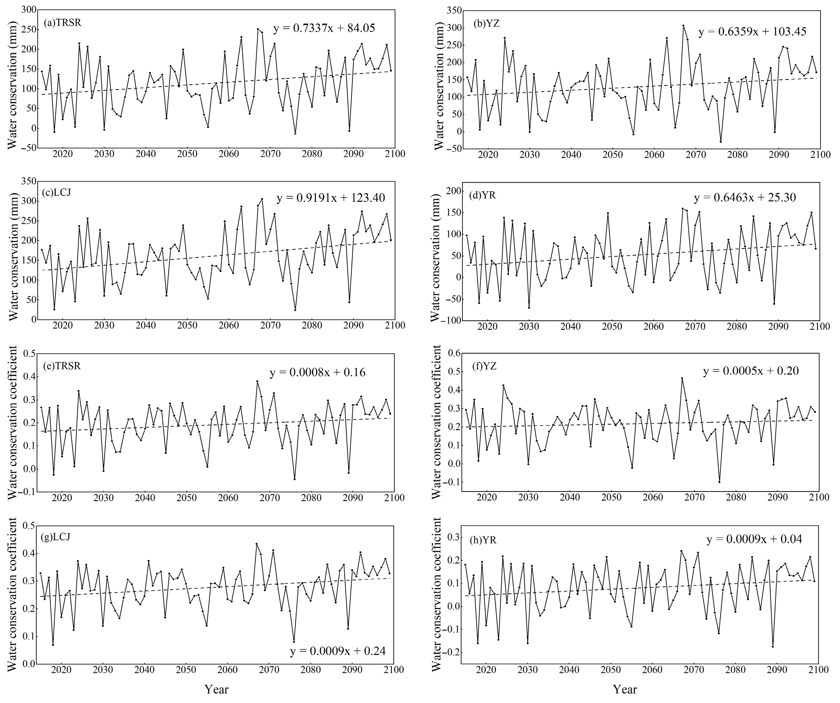
In different emission scenarios for the future, the water conservation capacity and water conservation coefficient of the TRSR showed different changes. In the SSP119 scenario, the water conservation capacity and water conservation coefficient of the TRSR and its three sub-regions showed an initial decreasing trend and then an increasing trend. In the SSP245 scenario, the water conservation capacity and water conservation coefficient of the TRSR and its three sub-regions first showed an upward trend and then a downward trend. In the SSP585 scenario, the trends of water conservation capacity and water conservation coefficient in the TRSR and its three sub-regions were significantly higher, with the most obvious increase being in the long-term, when the growth slope of water conservation reached about 5 mm/year, which is 10 times that of the near-term and 3~5 times that of the mid-term. The growth rate of water conservation coefficient was about 0.006/year in the long-term, which was 5–6 times that of the near- and mid-terms, while the growth rates in the mid- and long-terms were basically the same. For the different scenarios, the different measures should be adopted to protect the water conservation and the sustainable ecological development in the TRSR.
This study provides an important reference for ecological protection and water resource management in the region. Future studies can combine more actual observation data and advanced models such as an improved version of the SWAT model (SWAT+) for a comprehensive analysis to further improve the simulation accuracy. For the impacts of climate change and human activities on water conservation function, more in-depth studies will be carried out in the future, especially for the assessment and responses of specific water conservation capacities under extreme climate events and different land use changes.

Author Contributions

Conceptualization, Z.D. and J.L.; methodology, Z.L.; software, Z.L.; validation, W.Z., H.S., X.T. and H.M.; formal analysis, Z.L. and W.Z.; investigation, Z.L. and H.S.; writing—original draft preparation, Z.L.; writing—review and editing, W.Z., H.S., X.T. and H.M.; supervision, Z.L. and J.L. All authors have read and agreed to the published version of the manuscript.

Funding

This research was funded by the Natural Science Foundation of Hunan Province (Grant No. 2023JJ30484) and the National Natural Science Foundation of China (Grant Nos. 42375040 and 42275021).

Institutional Review Board Statement

Not applicable.

Informed Consent Statement

Not applicable.

Data Availability Statement

The DEM dataset used in our work can be freely accessed at the Natioal National Science Data Center of the Qinghai–Tibet Plateau: https://data.tpdc.ac.cn/home (accessed on 1 March 2023). The soil data can be freely accessed at Applied Systems Analysis (IIASA) World Harmonized Soil Database from the United Nations Food and Agriculture Organization (FAO) and the Vienna International Institute: HWSD: https://www.fao.org/home/en/ (accessed on 10 March 2023). The meteorological data can be freely accessed at the China Meteorological Administration: (https://data.cma.cn (accessed on 1 May 2023)).

Conflicts of Interest

The authors declare no conflicts of interest.

References

  1. Vörösmarty, C.J.; Green, P.; Salisbury, J.; Lammers, R.B. Global Water Resources: Vulnerability from Climate Change and Population Growth. Science 2000, 289, 284–288. [Google Scholar] [CrossRef] [PubMed]
  2. Sun, L.; Zhu, J. Comprehensive Benefit Study and Evaluation of Soil and Water Conservation Forest System; China Science and Technology Press: Beijing, China, 1995. [Google Scholar]
  3. Zhang, B.; Li, W.; Xie, G.; Xiao, Y. Water conservation function and its measurement methods of forest ecosystem. Chin. J. Ecol. 2009, 28, 529–534. (In Chinese) [Google Scholar]
  4. Deng, K.; Shi, P.; Xie, G. Water conservation of forest ecosystem in the upper reaches of yangtze river and its benefits. Resour. Sci. 2002, 24, 68–73. (In Chinese) [Google Scholar]
  5. Wei, C. Assessment and Comparative Study on the Changes of Water Conservation Function in Songjiang and Baihe Small Watersheds; Northeast Normal University: Changchun, China, 2021; (In Chinese). [Google Scholar] [CrossRef]
  6. Wang, Y.; Ye, A.; Qiao, F.; Li, Z.; Miao, C.; Di, Z.; Gong, W. Overview of the connotation and estimation methods of water conservation function. South-North Water Transf. Water Sci. Technol. 2021, 19, 1041–1071. [Google Scholar] [CrossRef]
  7. Akoko, G.; Le, T.H.; Gomi, T.; Kato, T. A review of SWAT model application in Africa. Water 2021, 13, 1313. [Google Scholar] [CrossRef]
  8. Shrestha, S.; Shrestha, M.; Shrestha, P.K. Evaluation of the SWAT model performance for simulating river discharge in the Himalayan and tropical basins of Asia. Hydrol. Res. 2018, 49, 846–860. [Google Scholar] [CrossRef]
  9. Sok, T.; Oeurng, C.; Ich, I.; Sauvage, S.; Miguel Sánchez-Pérez, J. Assessment of hydrology and sediment yield in the Mekong river basin using SWAT model. Water 2020, 12, 3503. [Google Scholar] [CrossRef]
  10. Martínez-Salvador, A.; Millares, A.; Eekhout, J.P.C.; Conesa-García, C. Assessment of streamflow from EURO-CORDEX regional climate simulations in semi-Arid catchments using the SWAT model. Sustainability 2021, 13, 7120. [Google Scholar] [CrossRef]
  11. Abbaspour, K.C.; Rouholahnejad, E.; Vaghefi, S.A.; Srinivasan, R.; Yang, H.; Kløve, B. A continental-scale hydrology and water quality model for Europe: Calibration and uncertainty of a high-resolution large-scale SWAT model. J. Hydrol. 2015, 524, 733–752. [Google Scholar] [CrossRef]
  12. Chien, H.; Yeh, P.J.; Knouft, J.H. Modeling the potential impacts of climate change on streamflow in agricultural watersheds of the Midwestern United States. J. Hydrol. 2013, 491, 73–88. [Google Scholar] [CrossRef]
  13. Chen, Y.; Feng, Q.; Wang, K. Research on the impact of pollution control measures on the improvement of Mangxi River water quality based on SWAT model. Sichuan Environ. 2024, 43, 24–31. (In Chinese) [Google Scholar] [CrossRef]
  14. Tai, L.; Rao, W.; Tan, T.; Tan, H.; Jiang, S.; Zhang, X. Scenario simulation study of hydrological characteristics in the Golmud river basin based on SWAT model. J. China Hydrol. 2023, 43, 46–51. (In Chinese) [Google Scholar] [CrossRef]
  15. Ma, X.; Wu, T.; Yu, Y. A study of runoff scenario prediction in the upper reaches of Hanjiang River based on SWAT model. Remote Sens. Nat. Resour. 2021, 1, 174–182. (In Chinese) [Google Scholar] [CrossRef]
  16. Zhou, D. Study on the Response of Runoff in the Upper Minjiang River Basin to Land Use and Climate Change over the Past 40 Years; Sichuan Agricultural University: Ya’an, China, 2019; (In Chinese). [Google Scholar] [CrossRef]
  17. Guo, W. Study on the Temporal and Spatial Variation of Nitrogen and Phosphorus Non-Point Source Pollution in Farmland Based on SWAT Model; North China University of Water Resources and Electric Power: Zhengzhou, China, 2019. [Google Scholar]
  18. Zhao, L. Simulation Study on Runoff and Sediment Yield in the Upstream of Huangqian Reservoir Based on SWAT Model; Shandong Agricultural University: Tai’an, China, 2022. [Google Scholar]
  19. Liu, Y.; Wang, W.; Liu, Y.; Cui, W. Data assimilation experiment of soil moisture based on EnKF method and SWAT model. Eng. J. Wuhan Univ. 2024, 57, 17–27. [Google Scholar] [CrossRef]
  20. Chen, Y.; Marek, G.W.; Marek, T.H.; Porter, D.O.; Brauer, D.K. Simulating the effects of agricultural production practices on water conservation and crop yields using an improved SWAT model in the Texas High Plains, USA. Agric. Water Manag. 2021, 244, 106574. [Google Scholar] [CrossRef]
  21. Li, C.; Zhang, X.; Wu, Y.; Hao, F.; Yin, G. Landscape pattern change of the ecological barrier zone in Beijing-Tianjin-Hebei region and its impact on water conservation. China Environ. Sci. 2019, 39, 2588–2595. (In Chinese) [Google Scholar]
  22. Lin, F.; Chen, X.; Yao, W.; Fang, Y.; Deng, H.; Wu, J.; Liu, B. Multi-time scale analysis of water conservation in a discontinuous forest watershed based on SWAT model. Acta Geogr. Sin. 2020, 75, 1065–1078. (In Chinese) [Google Scholar] [CrossRef]
  23. Li, M.; Di, Z.; Yao, Y.; Ma, Q. Variations in water conservation function and attributions in the Three-River Source Region of the Qinghai–Tibet Plateau based on the SWAT model. Agric. For. Meteorol. 2024, 349, 109956. [Google Scholar] [CrossRef]
  24. IPCC. 2023: Sections. In Climate Change 2023: Synthesis Report. Contribution of Working Groups I, II and III to the Sixth Assessment Report of the Intergovernmental Panel on Climate Change; Core Writing Team, Lee, H., Romero, J., Eds.; IPCC: Geneva, Switzerland, 2023; pp. 35–115. [Google Scholar] [CrossRef]
  25. Jensen, M.E.; Burman, R.D.; Allen, R.G. Evapotranspiration and Irrigation Water Requirements; American Society of Civil Engineers: New York, NY, USA, 1990; 360p. [Google Scholar]
  26. Priestley, C.H.B.; Taylor, R.J. On the assessment of surface heat flux and evaporation using large-scale parameters. Mon. Weather Rev. 1972, 100, 81–92. [Google Scholar] [CrossRef]
  27. Hargreaves, G.L.; Hargreaves, G.H.; Riley, J.P. Agricultural benefits for Senegal River Basin. J. Irrig. Drain. Eng. 1985, 111, 113–124. [Google Scholar] [CrossRef]
  28. Grusson, Y.G.; Sun, X.L.; Gascoin, S.; Sauvage, S.; Raghavan, S.; Anctil, F.; Sáchez-Pérez, J.M. Assessing the capability of the SWAT model to simulate snow, snow melt and streamflow dynamics over an alpine watershed. J. Hydrol. 2015, 531, 574–588. [Google Scholar] [CrossRef]
  29. Song, Z.; Zeng, J.; Jin, Y.; Hu, X.; Sun, D.; Lu, S.; Zhang, Y. Distributed simulation of monthly runoff using SWAT and SUFI-2 algorithm in Shiyang river basin. J. Soil Water Conserv. 2016, 36, 172–177. (In Chinese) [Google Scholar] [CrossRef]
  30. Liu, Y.; Lu, Y.; Zhou, Q.; Li, C. Application of HBV model to the study on risk precipitation in different grades in Batang river region. Res. Soil Water Conserv. 2015, 22, 5. (In Chinese) [Google Scholar] [CrossRef]
  31. Zhang, X.; Srinivasan, R.; Debele, B.; Hao, F. Runoff simulation of the headwaters of the Yellow River using the SWAT model with three snowmelt algorithms. J. Am. Water Resour. AS. 2008, 44, 48–61. [Google Scholar] [CrossRef]
  32. Zhang, Y.; Zhang, S.; Xia, J.; Dong, H. Temporal and spatial variation of the main water balance components in the three rivers source region, China from 1960 to 2000. Environ. Earth Sci. 2013, 68, 973–983. [Google Scholar] [CrossRef]
  33. Li, X.; Jia, H.; Chen, Y.; Wen, J. Runoff simulation and projection in the source area of the Yellow River using the SWAT model and SSPs scenarios. Front. Environ. Sci. 2022, 10, 1012838. [Google Scholar] [CrossRef]
  34. Liu, W.; Xu, Z.; Li, F.; Zhang, L.; Zhao, J.; Yang, H. Impacts of climate change on hydrological processes in the Tibetan Plateau: A case study in the Lhasa River basin. J. Am. Water Resour. Assoc. 2015, 29, 1809–1822. [Google Scholar] [CrossRef]
  35. Zhang, Y.; Zhang, S.; Zhai, X.; Xia, J. Runoff variation and its response to climate change in the Three Rivers Source Region. J. Geogr. Sci. 2012, 22, 781–794. [Google Scholar] [CrossRef]
  36. Zhang, F.; Yang, L.; Wang, C.; Zhang, C.; Wan, J. Distribution and conservation of plants in the northeastern Qinghai–Tibet Plateau under climate change. Diversity 2022, 14, 956. [Google Scholar] [CrossRef]
  37. He, Q.; Kuang, X.; Ma, E.; Chen, J.; Feng, Y.; Zheng, C. Evolution of runoff components and groundwater discharge under rapid climate warming: Lhasa river basin, Tibetan Plateau. J. Hydrol. 2024, 628, 130556. [Google Scholar] [CrossRef]
Figure 1. Location and elevation of the Three-River Source Region (TRSR).
Atmosphere 15 00889 g001
Figure 2. The optimal monthly runoff simulations and the corresponding observations in TRSR: (a) Yangtze River source (YZ); (b) Lancangjing River source (LCJ); (c) Yellow River source (YR).
Atmosphere 15 00889 g002
Figure 3. Annual changes in water conservation capacity and water conservation coefficient from 1981 to 2014: (ad) are water conservation capacities; (eh) are water conservation coefficients.
Atmosphere 15 00889 g003
Figure 4. Spatial distributions of water conservation capacity and water conservation coefficient from 1981 to 2014: (a,b) annual average distribution of water conservation capacity and its growth rate, respectively; (c,d) annual average distribution of water conservation coefficient and its growth rate, respectively.
Atmosphere 15 00889 g004
Figure 5. Correlation between the main meteorological (precipitation and temperature) and hydrological (evapotranspiration and catchment amount) elements and water conservation index (water conservation and water conservation coefficient).* represents p < 0.05, ** represents p < 0.01, and *** represents p < 0.001.
Atmosphere 15 00889 g005
Figure 6. Inter-annual variation of water conservation capacity and water conservation coefficient of TRSR in the SSP119 scenario from 2015 to 2099: (a,e) for TRSR; (b,f) for YZ; (c,g) for LCJ; (d,h) for YR.
Atmosphere 15 00889 g006
Figure 7. Spatial distribution of water conservation capacity and water conservation coefficient of TRSR in the SSP119 scenario: (a,d) for near-term; (b,e) for mid-term; (c,f) for long-term.
Atmosphere 15 00889 g007
Figure 8. Inter-annual variations of water conservation capacity and water conservation coefficient of TRSR in the SSP245 scenario: (a,e) for TRSR; (b,f) for YZ; (c,g) for LCJ; (d,h) for YR.
Atmosphere 15 00889 g008
Figure 9. Spatial distribution of water conservation capacity and water conservation coefficient of TRSR in the SSP245 scenario: (a,d) for near-term; (b,e) for mid-term; (c,f) for long-term.
Atmosphere 15 00889 g009
Figure 10. Inter-annual variations of water conservation capacity and water conservation coefficient of TRSR in the SSP585 scenario: (a,e) for TRSR; (b,f) for YZ; (c,g) for LCJ; (d,h) for YR.
Atmosphere 15 00889 g010
Figure 11. Spatial distribution of water conservation capacity and water conservation coefficient of the TRSR in the SSP585 scenario: (a,d) for near-term; (b,e) for mid-term; (c,f) for long-term.
Atmosphere 15 00889 g011
Table 1. TRSR hydrological station information.
Station IDStation NameLongitudeLatitudeData Range
40100350Tangnaihai100.1535.51 January 1981 to 1 December 2019
60100700Zhimenda97.2532.991 January 1981 to 15 September 2019
90200100Changdu97.1831.1815 January 1981 to 15 December 2009
Table 2. Slope of growth of water conservation capacity and water conservation coefficient in different time periods in the SSP119 scenario.
Water Conservation Capacity (mm/Year)Water Conservation Coefficient
Near-TermMid-TermLong-TermNear-TermMid-TermLong-Term
Three-River Source Region (TRSR)1.4091−0.10892.26810.0024−0.00020.0025
Yangtze River Source (YZ)0.838−0.16951.76630.0054−0.00050.0054
Lancangjing River Source (LCJ)0.59940.10041.11680.001−0.00030.0011
Yellow River Source (YR)2.7897−0.25763.92120.00080.00030.001
Table 3. Slope of growth of water conservation capacity and water conservation coefficients for different time periods in the SSP245 scenario.
Water Conservation Capacity (mm/Year)Water Conservation Coefficient
Near-TermMid-TermLong-TermNear-TermMid-TermLong-Term
TRSR1.00662.217−0.08540.0020.002−0.0007
YZ1.07512.7391−2.74370.0020.0025−0.0032
LCJ1.16822.3827−2.37490.00190.0015−0.002
YR 0.77641.5293−0.61270.00210.0021−0.0021
Table 4. Growth slope of water conservation capacity and water conservation coefficient at different times in the SSP585 scenario.
Water Conservation Capacity (mm/Year)Water Conservation Coefficient
Near-TermMid-TermLong-TermNear-TermMid-TermLong-Term
TRSR0.31651.7684.98390.0010.00120.0064
YZ0.21471.57565.28280.00080.00060.0068
LCJ0.63182.46825.65280.00140.00170.0061
YR 0.1031.264.01610.00090.00140.0061
Disclaimer/Publisher’s Note: The statements, opinions and data contained in all publications are solely those of the individual author(s) and contributor(s) and not of MDPI and/or the editor(s). MDPI and/or the editor(s) disclaim responsibility for any injury to people or property resulting from any ideas, methods, instructions or products referred to in the content.

