
Parameter Study of Geoeffective Active Regions


Abstract
:1. Introduction
2. Data and Event Sample
- USFLUX: Total unsigned flux [Mx];
- MEANGAM: Mean inclination angle, [degrees];
- MEANGBT: Mean value of the total field gradient [G/Mm];
- MEANGBZ: Mean value of the vertical field gradient [G/Mm];
- MEANGBH: Mean value of the horizontal field gradient [G/Mm];
- MEANJZD: Mean vertical current density [mA/m2];
- TOTUSJZ: Total unsigned vertical current [A];
- MEANALP: Mean twist parameter, [1/Mm];
- MEANJZH: Mean current helicity [G2/m];
- TOTUSJH: Total unsigned current helicity [G2/m];
- ABSNJZH: Absolute value of the net current helicity [G2/m];
- SAVNCPP: Sum of the absolute value of the net currents [A];
- MEANPOT: Mean photospheric excess magnetic energy density [Ergs/cm3];
- TOTPOT: Total photospheric magnetic energy density [Ergs/cm3];
- MEANSHR: Mean shear angle for Btotal [degrees];
- RVALUE: Unsigned flux, R [35] [Mx].
3. Results
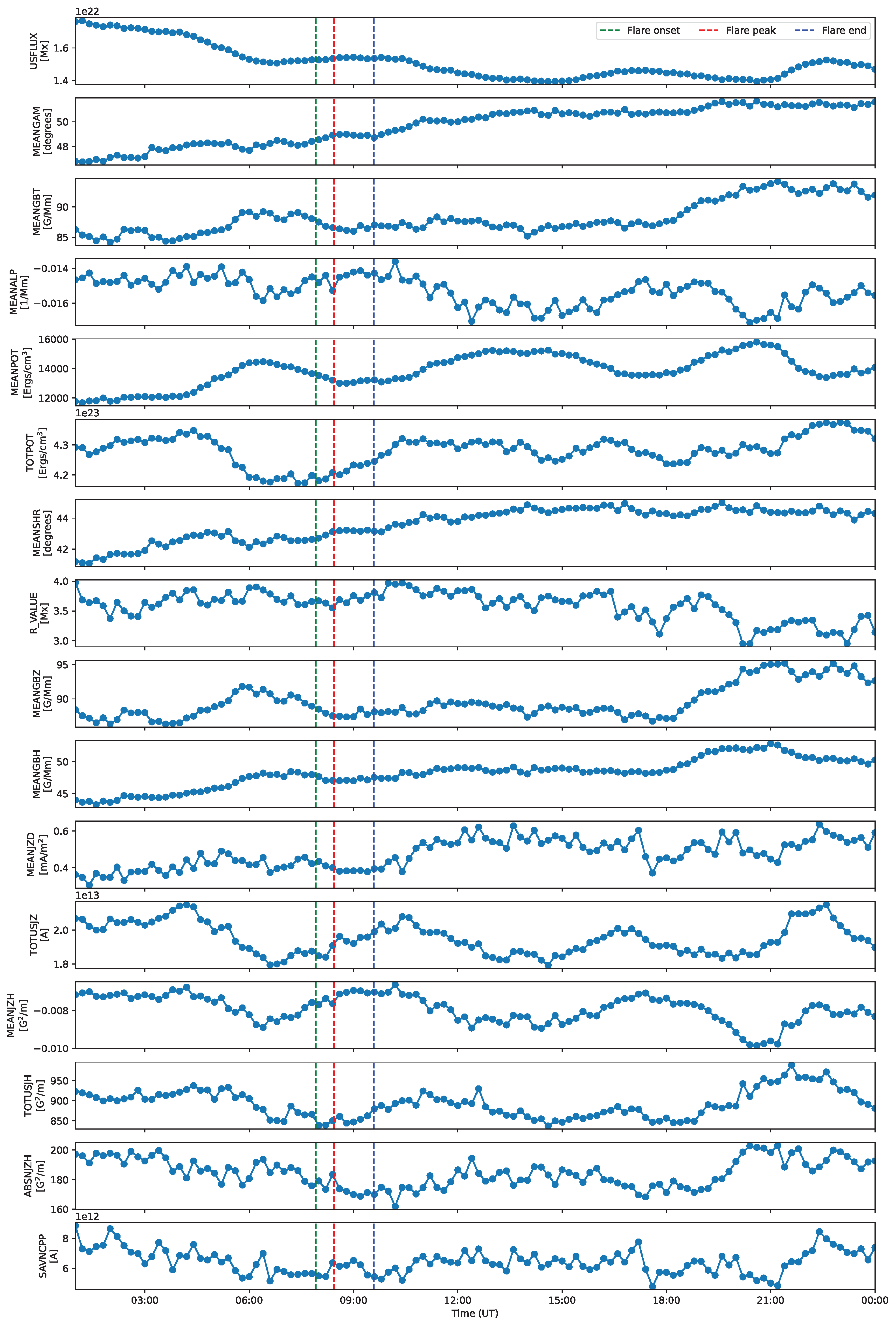
3.1. Timing Estimation
- An exact value taken just prior to the SF start;
- Averaged value during the rise phase of the SF (onset-to-peak);
- Averaged value during the entire SF duration (onset-to-end);
- Averaged value during the decline phase of the SF (peak-to-end).
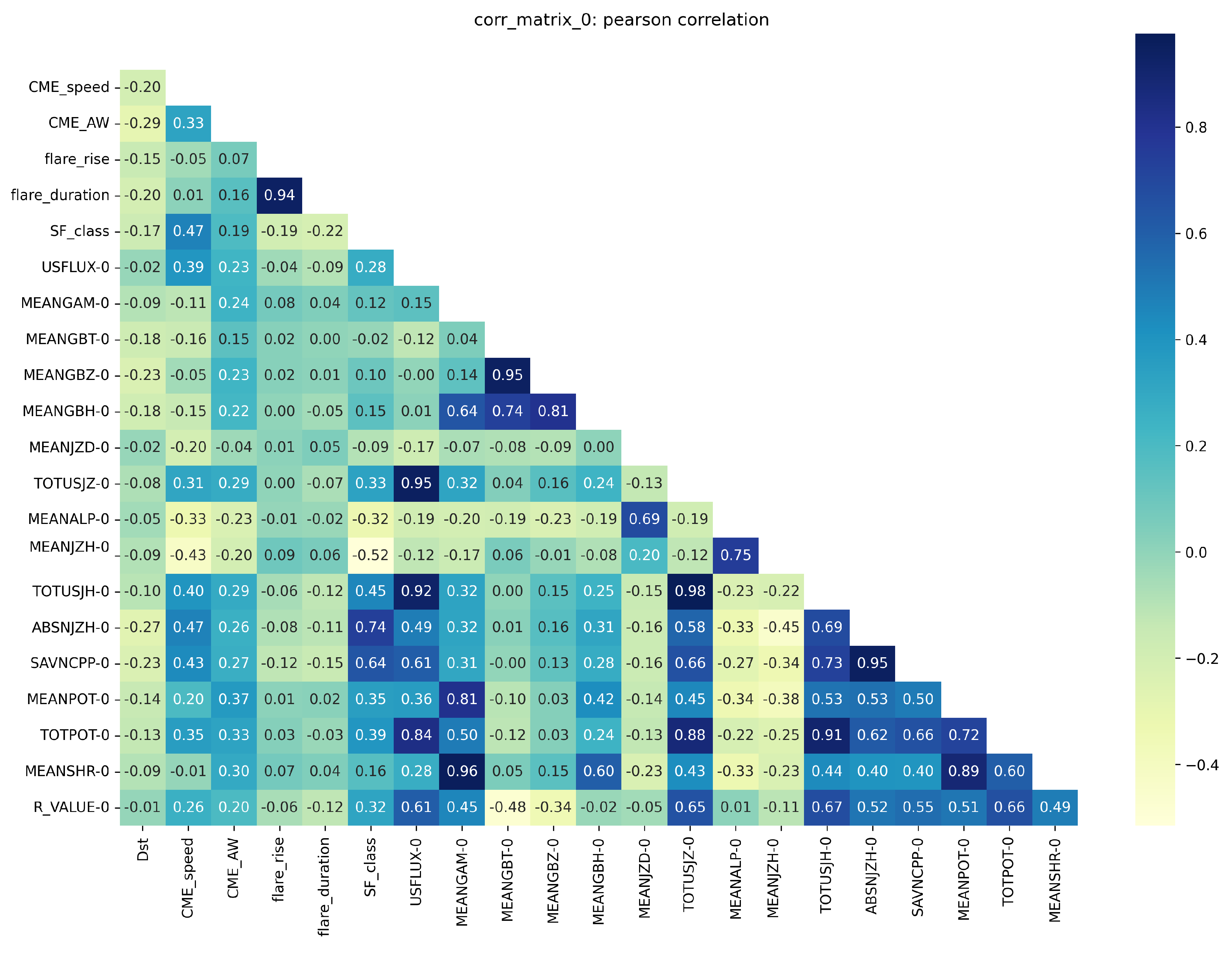
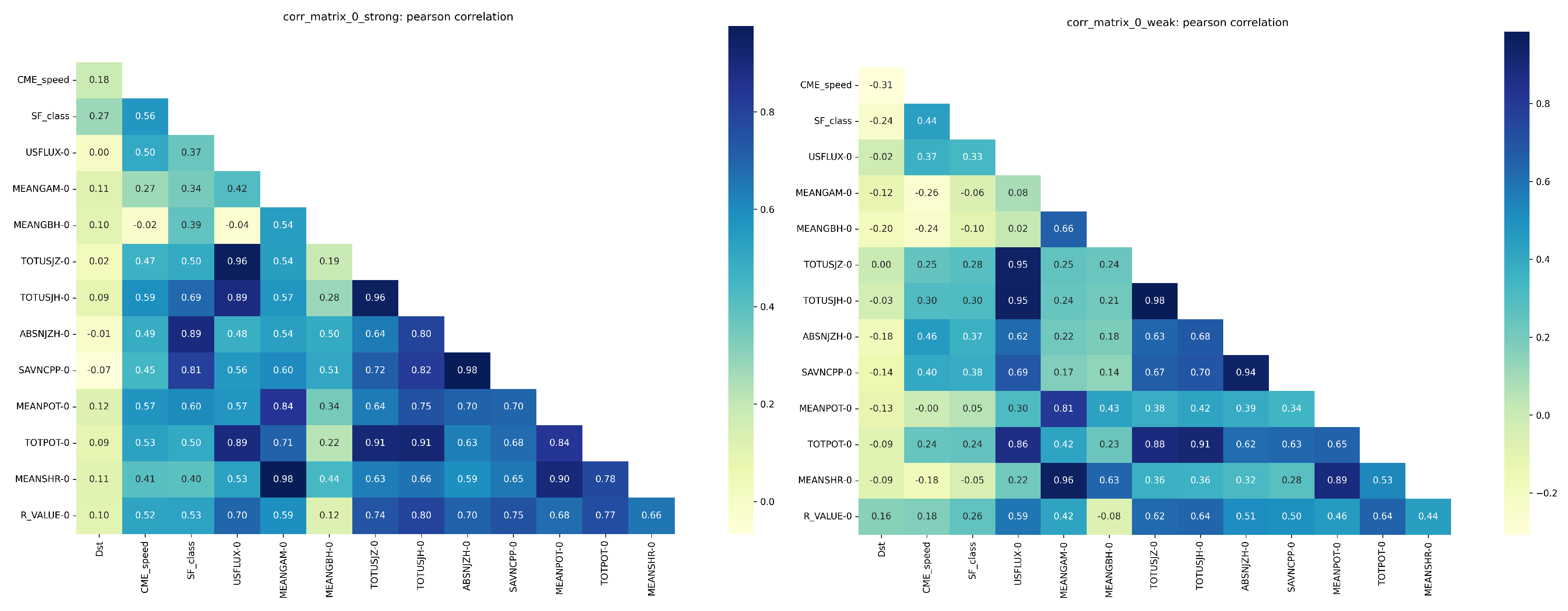
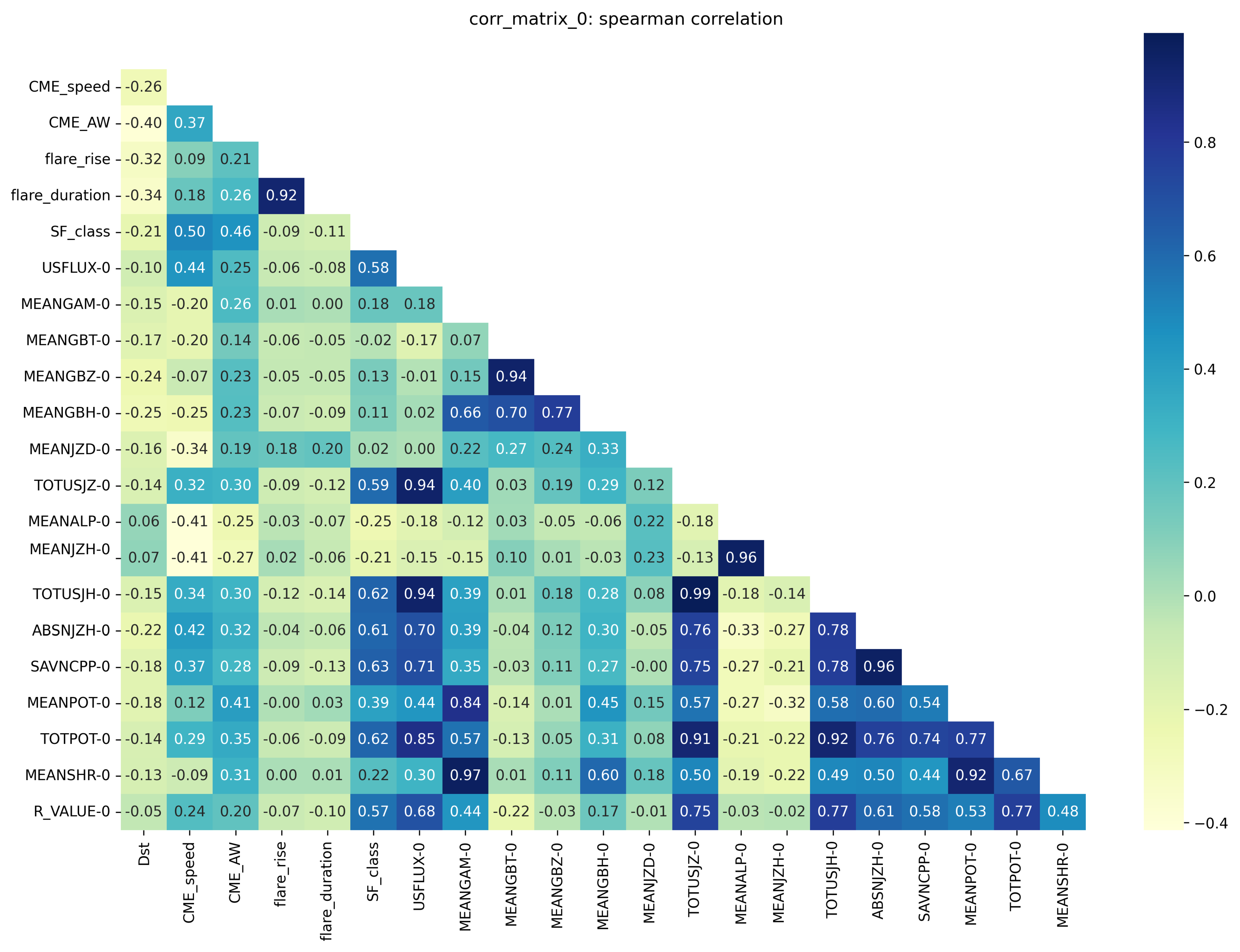
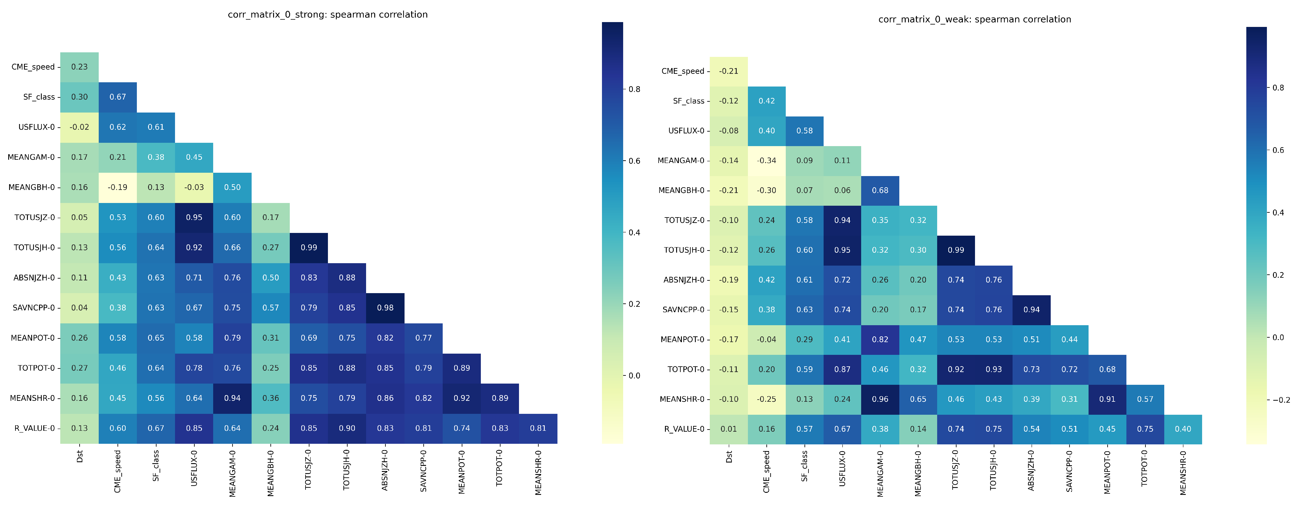
3.2. Correlations
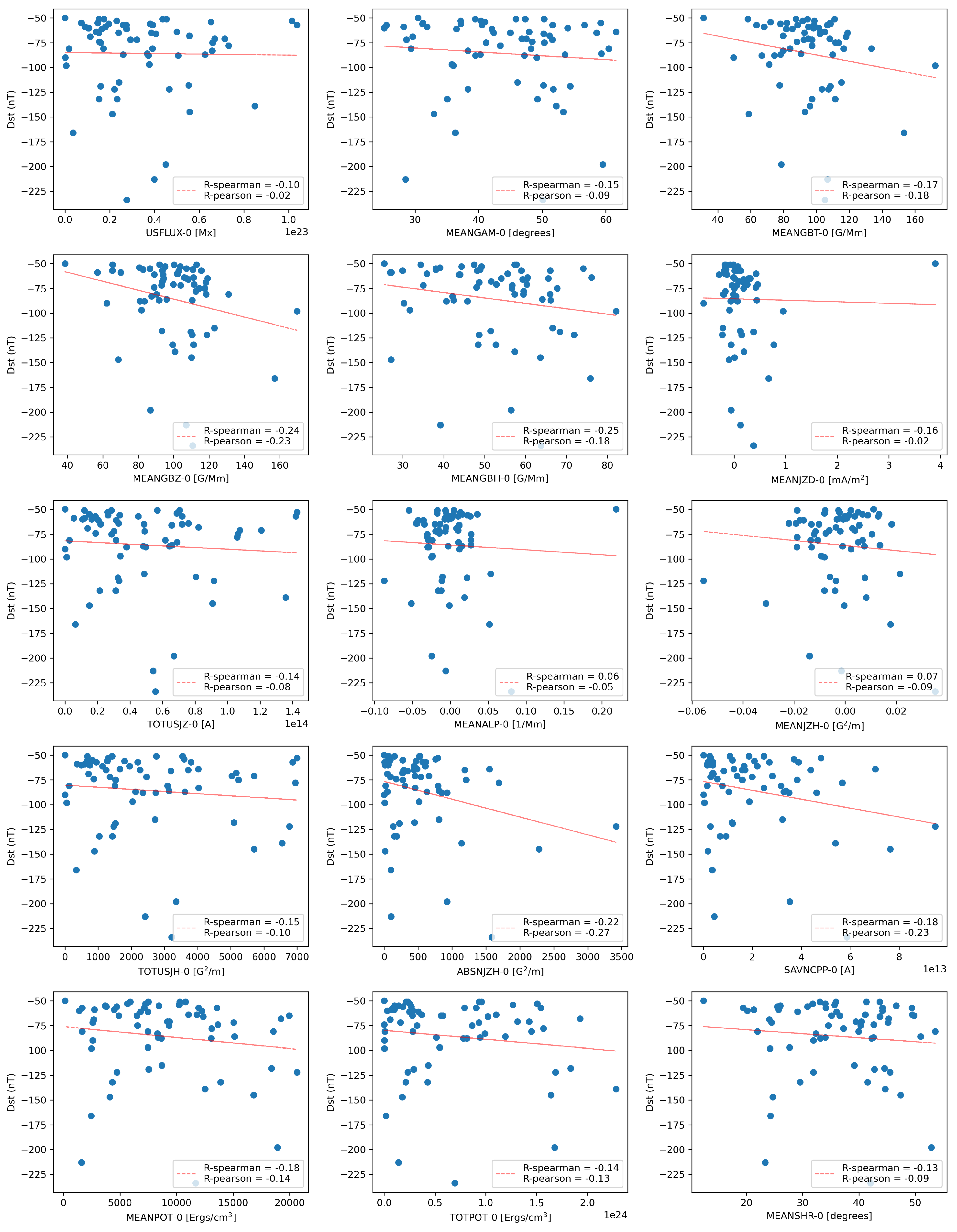
3.3. Scatter Plots
- Dst vs. MEANGBT: ();
- Dst vs. MEANGBZ: ();
- Dst vs. MEANJZD: ();
- Dst vs. MEANAPL: ();
- Dst vs. ABSNJZH: (),
4. Discussion
5. Conclusions
- The mean (median) value of the Dst index of our sample of GSs is −86 (−72) nT, which is similar to the respective value over the last two SCs −86 (−69) nT [37].
- The GS-associated CMEs are slower with the mean (median) projected speed of ∼750 (620) km s−1, compared to the ∼1000 (870) km s−1 values reported by [37] over SC23+24.
- The GS-associated SFs have larger mean SXR flux of M6.9 compared to M1.5 reported by [37] over SC23+24, although the median value is nearly the same.
- Selected SHARP (MEANGBT, MEANGBZ, MEANJZD, MEANALP, and MEANJZH) and solar (flare rise and duration) parameters show weak or negative statistical correlations with the other SHARP or solar parameters, apart from a few strong inter-correlations.
- The remaining SHARP parameters (USFLUX, MEANGAM, MEANGBH, TOTUSJZ, TOTUSJH, ABSNJZH, SAVNCPP, MEANPOT, TOTPOT, and MEANSHR) show moderate-to-strong correlations with the SF class (but not to the rise and duration times) and to a degree also with the CME speed and AW, whereas no correlation is found with the Dst index of the GSs. The latter correlation trend is improved slightly when considering strong GSs (with Dst ≤ −100 nT).
- The weak correlations with the GSs are not improved after the removal of outliers from the event samples.
Supplementary Materials
Author Contributions
Funding
Institutional Review Board Statement
Informed Consent Statement
Data Availability Statement
Conflicts of Interest
Abbreviations
| AR | active region |
| AW | angular width |
| CDAW | Coordinated Data Analysis Workshop |
| CME | coronal mass ejection |
| Dst | disturbance storm time |
| EM | electromagnetic |
| GOES | Geostationary Operational Environmental Satellite |
| GS | geomagnetic storm |
| HMI | Helioseismic and Magnetic Imager |
| ICME | interplanetary coronal mass ejection |
| IMF | interplanetary magnetic field |
| IP | interplanetary |
| PIL | polarity inversion line |
| LASCO | Large Angle and Spectrometric COronagraph |
| NOAA | National Oceanic and Atmospheric Administration |
| SC | solar cycle |
| SDO | Solar Dynamics Observatory |
| SEE | solar energetic electron |
| SEP | solar energetic proton |
| SF | solar flare |
| SHARP | Space-weather HMI Active Region Patch |
| SN | sunspot number |
| SOHO | Solar and Heliospheric Observatory |
| SR | sunspot region |
| SXR | soft X-ray |
| SW | space weather |
| UT | universal time |
Appendix A. Pearson Correlation Coefficients
References
- van Driel-Gesztelyi, L.; Green, L.M. Evolution of Active Regions. Living Rev. Sol. Phys. 2015, 12, 1. [Google Scholar] [CrossRef]
- Fletcher, L.; Dennis, B.R.; Hudson, H.S.; Krucker, S.; Phillips, K.; Veronig, A.; Battaglia, M.; Bone, L.; Caspi, A.; Chen, Q.; et al. An Observational Overview of Solar Flares. Space Sci. Rev. 2011, 159, 19–106. [Google Scholar] [CrossRef]
- Benz, A.O. Flare Observations. Living Rev. Sol. Phys. 2017, 14, 2. [Google Scholar] [CrossRef]
- Webb, D.F.; Howard, T.A. Coronal Mass Ejections: Observations. Living Rev. Sol. Phys. 2012, 9, 3. [Google Scholar] [CrossRef]
- Green, L.M.; Török, T.; Vršnak, B.; Manchester, W.; Veronig, A. The Origin, Early Evolution and Predictability of Solar Eruptions. Space Sci. Rev. 2018, 214, 46. [Google Scholar] [CrossRef]
- Klein, K.L.; Dalla, S. Acceleration and Propagation of Solar Energetic Particles. Space Sci. Rev. 2017, 212, 1107–1136. [Google Scholar] [CrossRef]
- Pulkkinen, T. Space Weather: Terrestrial Perspective. Living Rev. Sol. Phys. 2007, 4, 1. [Google Scholar] [CrossRef]
- Koskinen, H.E.J.; Baker, D.N.; Balogh, A.; Gombosi, T.; Veronig, A.; von Steiger, R. Achievements and Challenges in the Science of Space Weather. Space Sci. Rev. 2017, 212, 1137–1157. [Google Scholar] [CrossRef]
- Temmer, M. Space weather: The solar perspective. Living Rev. Sol. Phys. 2021, 18, 4. [Google Scholar] [CrossRef]
- Miteva, R.; Samwel, S.W.; Tkatchova, S. Space Weather Effects on Satellites. Astronomy 2023, 2, 165–179. [Google Scholar] [CrossRef]
- Kolarski, A.; Veselinović, N.; Srećković, V.A.; Mijić, Z.; Savić, M.; Dragić, A. Impacts of Extreme Space Weather Events on September 6th, 2017 on Ionosphere and Primary Cosmic Rays. Remote Sens. 2023, 15, 1403. [Google Scholar] [CrossRef]
- Kilpua, E.; Koskinen, H.E.J.; Pulkkinen, T.I. Coronal mass ejections and their sheath regions in interplanetary space. Living Rev. Sol. Phys. 2017, 14, 5. [Google Scholar] [CrossRef] [PubMed]
- Semkova, J.; Koleva, R.; Benghin, V.; Dachev, T.; Matviichuk, Y.; Tomov, B.; Krastev, K.; Maltchev, S.; Dimitrov, P.; Mitrofanov, I.; et al. Charged particles radiation measurements with Liulin-MO dosimeter of FREND instrument aboard ExoMars Trace Gas Orbiter during the transit and in high elliptic Mars orbit. Icarus 2018, 303, 53–66. [Google Scholar] [CrossRef]
- Hands, A.D.P.; Ryden, K.A.; Meredith, N.P.; Glauert, S.A.; Horne, R.B. Radiation Effects on Satellites During Extreme Space Weather Events. Space Weather 2018, 16, 1216–1226. [Google Scholar] [CrossRef]
- Miteva, R.; Samwel, S.W.; Costa-Duarte, M.V.; Malandraki, O.E. Solar cycle dependence of Wind/EPACT protons, solar flares and coronal mass ejections. Sun Geosph. 2017, 12, 11–19. [Google Scholar]
- Altschuler, M.D.; Newkirk, G. Magnetic Fields and the Structure of the Solar Corona. I: Methods of Calculating Coronal Fields. Sol. Phys. 1969, 9, 131–149. [Google Scholar] [CrossRef]
- Scherrer, P.H.; Schou, J.; Bush, R.I.; Kosovichev, A.G.; Bogart, R.S.; Hoeksema, J.T.; Liu, Y.; Duvall, T.L.; Zhao, J.; Title, A.M.; et al. The Helioseismic and Magnetic Imager (HMI) Investigation for the Solar Dynamics Observatory (SDO). Sol. Phys. 2012, 275, 207–227. [Google Scholar] [CrossRef]
- Contopoulos, I. The Force-Free Electrodynamics Method for the Extrapolation of Coronal Magnetic Fields from Vector Magnetograms. Sol. Phys. 2013, 282, 419–426. [Google Scholar] [CrossRef]
- Wiegelmann, T.; Thalmann, J.K.; Inhester, B.; Tadesse, T.; Sun, X.; Hoeksema, J.T. How Should One Optimize Nonlinear Force-Free Coronal Magnetic Field Extrapolations from SDO/HMI Vector Magnetograms? Sol. Phys. 2012, 281, 37–51. [Google Scholar] [CrossRef]
- Jarolim, R.; Thalmann, J.K.; Veronig, A.M.; Podladchikova, T. Probing the solar coronal magnetic field with physics-informed neural networks. Nat. Astron. 2023, 7, 1171–1179. [Google Scholar] [CrossRef]
- Parker, E.N. Dynamics of the Interplanetary Gas and Magnetic Fields. Astrophys. J. 1958, 128, 664. [Google Scholar] [CrossRef]
- Fisk, L.A.; Zurbuchen, T.H.; Schwadron, N.A. On the Coronal Magnetic Field: Consequences of Large-Scale Motions. Astrophys. J. 1999, 521, 868–877. [Google Scholar] [CrossRef]
- Owens, M.J.; Forsyth, R.J. The Heliospheric Magnetic Field. Living Rev. Sol. Phys. 2013, 10, 5. [Google Scholar] [CrossRef]
- Kilpua, E.K.J.; Balogh, A.; von Steiger, R.; Liu, Y.D. Geoeffective Properties of Solar Transients and Stream Interaction Regions. Space Sci. Rev. 2017, 212, 1271–1314. [Google Scholar] [CrossRef]
- Regnault, F.; Strugarek, A.; Janvier, M.; Auchère, F.; Lugaz, N.; Al-Haddad, N. Eruption and propagation of twisted flux ropes from the base of the solar corona to 1 au. Astron. Astrophys. 2023, 670, A14. [Google Scholar] [CrossRef]
- Sarkar, R.; Pomoell, J.; Kilpua, E.; Asvestari, E.; Wijsen, N.; Maharana, A.; Poedts, S. Studying the Spheromak Rotation in Data-constrained Coronal Mass Ejection Modeling with EUHFORIA and Assessing Its Effect on the Bz Prediction. Astrophys. J. 2024, 270, 18. [Google Scholar] [CrossRef]
- Akasofu, S.I. A Historical Review of the Geomagnetic Storm-Producing Plasma Flows from the Sun. Space Sci. Rev. 2011, 164, 85–132. [Google Scholar] [CrossRef]
- Gonzalez, W.D.; Joselyn, J.A.; Kamide, Y.; Kroehl, H.W.; Rostoker, G.; Tsurutani, B.T.; Vasyliunas, V.M. What is a geomagnetic storm? J. Geophys. Res. 1994, 99, 5771–5792. [Google Scholar] [CrossRef]
- Lassen, K.; Sharber, J.R.; Winningham, J.D. The development of auroral and geomagnetic substorm activity after a southward turning of the interplanetary magnetic field following several hours of magnetic calm. J. Geophys. Res. 1977, 82, 5031. [Google Scholar] [CrossRef]
- Kay, C.; Gopalswamy, N. The Effects of Uncertainty in Initial CME Input Parameters on Deflection, Rotation, Bz, and Arrival Time Predictions. J. Geophys. Res. (Space Phys.) 2018, 123, 7220–7240. [Google Scholar] [CrossRef]
- Manchester, W.; Kilpua, E.K.J.; Liu, Y.D.; Lugaz, N.; Riley, P.; Török, T.; Vršnak, B. The Physical Processes of CME/ICME Evolution. Space Sci. Rev. 2017, 212, 1159–1219. [Google Scholar] [CrossRef]
- Zhou, Z.; Jiang, C.; Liu, R.; Wang, Y.; Liu, L.; Cui, J. The Rotation of Magnetic Flux Ropes Formed during Solar Eruption. Astrophys. J. 2022, 927, L14. [Google Scholar] [CrossRef]
- Schrijver, C.J.; De Rosa, M.L. Photospheric and heliospheric magnetic fields. Sol. Phys. 2003, 212, 165–200. [Google Scholar] [CrossRef]
- Bobra, M.G.; Sun, X.; Hoeksema, J.T.; Turmon, M.; Liu, Y.; Hayashi, K.; Barnes, G.; Leka, K.D. The Helioseismic and Magnetic Imager (HMI) Vector Magnetic Field Pipeline: SHARPs - Space-Weather HMI Active Region Patches. Sol. Phys. 2014, 289, 3549–3578. [Google Scholar] [CrossRef]
- Schrijver, C.J. A Characteristic Magnetic Field Pattern Associated with All Major Solar Flares and Its Use in Flare Forecasting. Astrophys. J. 2007, 655, L117–L120. [Google Scholar] [CrossRef]
- Kane, R.P. How good is the relationship of solar and interplanetary plasma parameters with geomagnetic storms? J. Geophys. Res. (Space Phys.) 2005, 110, A02213. [Google Scholar] [CrossRef]
- Miteva, R.; Samwel, S.W. Catalog of Geomagnetic Storms with Dst Index ≤ -50 nT and Their Solar and Interplanetary Origin (1996–2019). Atmosphere 2023, 14, 1744. [Google Scholar] [CrossRef]
- Cane, H.V.; Richardson, I.G. Interplanetary coronal mass ejections in the near-Earth solar wind during 1996–2002. J. Geophys. Res. (Space Phys.) 2003, 108, 1156. [Google Scholar] [CrossRef]
- Richardson, I.G.; Cane, H.V. Near-Earth Interplanetary Coronal Mass Ejections During Solar Cycle 23 (1996–2009): Catalog and Summary of Properties. Sol. Phys. 2010, 264, 189–237. [Google Scholar] [CrossRef]
- Gopalswamy, N.; Yashiro, S.; Michalek, G.; Stenborg, G.; Vourlidas, A.; Freeland, S.; Howard, R. The SOHO/LASCO CME Catalog. Earth Moon Planets 2009, 104, 295–313. [Google Scholar] [CrossRef]
- Guerra, J.A.; Park, S.H.; Gallagher, P.T.; Kontogiannis, I.; Georgoulis, M.K.; Bloomfield, D.S. Active Region Photospheric Magnetic Properties Derived from Line-of-Sight and Radial Fields. Sol. Phys. 2018, 293, 9. [Google Scholar] [CrossRef]
- Gao, P.X. Association of X-class flares with sunspot groups of various classes in Cycles 22 and 23. Mon. Not. R. Astron. Soc. 2019, 484, 5692–5701. [Google Scholar] [CrossRef]
- Miteva, R.; Samwel, S.W. M-Class Solar Flares in Solar Cycles 23 and 24: Properties and Space Weather Relevance. Universe 2022, 8, 39. [Google Scholar] [CrossRef]
- Wang, R.; Liu, Y.D.; Dai, X.; Yang, Z.; Huang, C.; Hu, H. The Role of Active Region Coronal Magnetic Field in Determining Coronal Mass Ejection Propagation Direction. Astrophys. J. 2015, 814, 80. [Google Scholar] [CrossRef]
- Wang, J.; Hoeksema, J.T.; Liu, S. The Deflection of Coronal Mass Ejections by the Ambient Coronal Magnetic Field Configuration. J. Geophys. Res. (Space Phys.) 2020, 125, e27530. [Google Scholar] [CrossRef]
- Li, T.; Liu, L.; Hou, Y.; Zhang, J. Two Types of Confined Solar Flares. Astrophys. J. 2019, 881, 151. [Google Scholar] [CrossRef]
- Gupta, M.; Thalmann, J.K.; Veronig, A.M. Stability of the coronal magnetic field around large confined and eruptive solar flares. Astron. Astrophys. 2024, 686, A115. [Google Scholar] [CrossRef]
- Chen, Y.; Manchester, W.B.; Hero, A.O.; Toth, G.; DuFumier, B.; Zhou, T.; Wang, X.; Zhu, H.; Sun, Z.; Gombosi, T.I. Identifying Solar Flare Precursors Using Time Series of SDO/HMI Images and SHARP Parameters. Space Weather 2019, 17, 1404–1426. [Google Scholar] [CrossRef]
- Lin, P.H.; Kusano, K.; Shiota, D.; Inoue, S.; Leka, K.D.; Mizuno, Y. A New Parameter of the Photospheric Magnetic Field to Distinguish Eruptive-flare Producing Solar Active Regions. Astrophys. J. 2020, 894, 20. [Google Scholar] [CrossRef]

| No. | GS | SR | CME | SF | |||||||
|---|---|---|---|---|---|---|---|---|---|---|---|
| yyyy-mm-dd | h | Dst | Type | Day/Onset | Speed | AW | Onset/Peak/End | Class | Location | AR | |
| 1 | 2010-08-04 | 2 | −74 | 01/13:42 | 850 | 360 | 07:55/08:26/09:35 | C3.2 | N20E36 | 11092 | |
| 2 | 2011-03-11 | 6 | −83 | 07/20:00 u | 2125 | 360 | 19:43/20:12/20:58 | M3.7 | N31W53 | 11164 | |
| 3 | 2011-08-06 | 4 | −115 | () | 04/04:12 | 1315 | 360 | 03:41/03:57/04:04 | M9.3 | N19W36 | 11261 |
| 4 | 2011-09-10 | 5 | −75 | () | 06/23:06 u | 575 | 360 | 22:12/22:20/22:24 | X2.1 | N14W18 | 11283 |
| 5 | 2011-09-26 | 24 | −118 | () | 24/12:48 | 1915 | 360 | 12:33/13:20/14:10 | M7.1 | N10E56 | 11302 |
| 6 | 2011-09-28 | 7 | −68 | () | 24/19:36 u | 972 | 360 | 19:09/19:21/19:41 | M3.0 | N12E42 | 11302 |
| 7 | 2011-10-25 | 2 | −147 | (no) | 22/10:24 | 1005 | 360 | 10:00/11:10/13:09 | M1.3 | N25W77 | 11314 |
| 8 | 2012-01-23 | 6 | −71 | 19/14:36 | 1120 | 360 | 13:44/16:05/17:50 | M3.2 | N32E22 | 11402 | |
| 9 | 2012-01-25 | 11 | −75 | 23/04:00 | 2175 | 360 | 03:38/03:59/04:34 | M8.7 | N28W21 | 11402 | |
| 10 | 2012-02-27 | 20 | −57 | () | 25/15:12 u | 1039 | 97 | 14:20/15:00/15:15 | B5.9 | N09E68 v | 11424 |
| 11 | 2012-03-04 | 2 | −50 | no | 02/18:00 u | 710 | 206 | 17:29/17:46/18:07 | M3.3 | N16E83 | 11429 |
| 12 | 2012-03-07 | 10 | −88 | () | 04/11:00 d | 1306 | 360 | 10:29/10:52/12:16 | M2.0 | N19E61 | 11429 |
| 13 | 2012-03-09 | 9 | −145 | 07/00:24 | 2684 | 360 | 00:02/00:24/00:40 | X5.4 | N17E27 | 11429 | |
| 14 | 2012-03-12 | 17 | −64 | 10/18:00 | 1296 | 360 | 17:15/17:44/18:30 | M8.4 | N17W24 | 11429 | |
| 15 | 2012-03-15 | 21 | −88 | 13/17:36 | 1884 | 360 | 17:12/17:41/18:25 | M7.9 | N17W66 | 11429 | |
| 16 | 2012-04-13 | 5 | −60 | no | 09/12:36 u | 921 | 360 | 12:12/12:44/13:08 | C3.9 | N20W65 | 11451 |
| 17 | 2012-06-17 | 14 | −86 | 14/14:12 u | 987 | 360 | 12:52/14:35/15:56 | M1.9 | S17E06 | 11504 | |
| 18 | 2012-07-09 | 13 | −78 | 06/23:24 u | 1828 | 360 | 23:01/23:08/23:14 | X1.1 | S13W59 | 11515 | |
| 19 | 2012-07-15 | 17 | −139 | 12/16:48 | 885 | 360 | 15:37/16:49/17:30 | X1.4 | S15W01 | 11520 | |
| 20 | 2012-09-03 | 11 | −69 | 31/20:00 u | 1442 | 360 | 19:45/20:43/21:51 | C8.4 | S19E42 | 11562 | |
| 21 | 2012-09-05 | 6 | −64 | 02/04:00 | 538 | 360 | 01:50/01:58/02:10 | C2.9 | N03W05 | 11560 | |
| 22 | 2012-10-01 | 5 | −122 | 28/00:12 | 947 | 360 | 23:36/23:57/00:34 | C3.7 | N06W34 | 11577 | |
| 23 | 2012-10-13 | 8 | −90 | no | 09/00:48 u | 692 | 122 | 23:56/01:06/02:01 | C2.0 | S26E86 | 11589 |
| 24 | 2013-03-01 | 11 | −55 | 27/04:00 u | 622 | 138 | 03:25/03:32/03:39 | B8.3 | S19W05 | 11682 | |
| 25 | 2013-03-17 | 21 | −132 | 15/07:12 | 1063 | 360 | 05:46/06:58/08:35 | X1.1 | N11E12 | 11692 | |
| 26 | 2013-03-29 | 17 | −59 | no () | 23/12:24 u | 663 | 177 | 12:15/12:22/12:27 | B6.8 | N17E87 u | 11704 |
| 27 | 2013-05-18 | 5 | −61 | 15/01:48 m | 1366 | 360 | 01:25/01:48/01:58 | X1.2 | N12E64 | 11748 | |
| 28 | 2013-05-19 | 15 | −51 | 17/09:12 | 1345 | 360 | 08:43/08:57/09:19 | M3.2 | N12E57 | 11748 | |
| 29 | 2013-05-25 | 7 | −59 | 22/13:26 | 1466 | 360 | 13:08/13:32/14:08 | M5.0 | N14W87 | 11745 | |
| 30 | 2013-07-06 | 19 | −87 | no () | 03/07:24 u | 807 | 267 | 07:00/07:08/07:18 | M1.5 | S11E82 | 11787 |
| 31 | 2013-10-02 | 8 | −72 | 29/22:12 | 1179 | 360 | 21:43/23:39/01:03 | C1.2 | N10W43 | 11850 v | |
| 32 | 2013-10-30 | 24 | −54 | 28/02:24 | 695 | 360 | 01:41/02:03/02:12 | X1.0 | N04W66 | 11875 | |
| 33 | 2014-02-19 | 9 | −119 | 16/10:00 | 634 | 360 | 09:20/09:26/09:29 | M1.1 | S11E01 | 11977 | |
| 34 | 2014-02-27 | 24 | −97 | 25/01:26 | 2147 | 360 | 00:39/00:49/01:03 | X4.9 | S12E82 | 11990 | |
| 35 | 2014-11-10 | 18 | −65 | 07/18:08 u | 795 | 293 | 16:53/17:26/17:34 | X1.6 | N15E33 | 12205 | |
| 36 | 2014-12-22 | 6 | −71 | 17/05:00 u | 587 | 360 | 04:25/04:51/05:20 | M8.7 | S20E09 | 12242 | |
| 37 | 2014-12-23 | 23 | −57 | 19/01:05 u | 1195 | 360 | 21:41/21:58/21:45 | M6.9 | S11E15 | 12242 | |
| 38 | 2014-12-24 | 23 | −53 | 20/01:26 u | 830 | 257 | 00:11/00:28/00:55 | X1.8 | S21W24 | 12242 | |
| 39 | 2014-12-26 | 2 | −57 | 21/12:12 u | 669 | 360 | 11:24/12:17/12:57 | M1.0 | S14W25 | 12241 | |
| 40 | 2015-03-17 | 23 | −234 | 15/01:48 | 719 | 360 | 01:15/02:13/03:20 | C9.1 | S22W25 | 12297 | |
| 41 | 2015-06-23 | 5 | −198 | 21/02:36 m | 1366 | 360 | 01:02/01:42/02:00 | M2.0 | N12E16 | 12371 | |
| 42 | 2015-06-25 | 17 | −81 | 22/18:36 d | 1209 | 360 | 17:39/18:23/18:51 | M6.5 | N12W08 | 12371 | |
| 43 | 2015-06-26 | 18 | −51 | 25/08:36 u | 1627 | 360 | 08:02/08:16/09:05 | M7.9 | N09W42 | 12371 | |
| 44 | 2015-08-16 | 8 | −98 | 12/14:48 u | 647 | 204 | 14:26/15:26/16:47 | B7.0 | S27W27 | 12399 v | |
| 45 | 2015-08-23 | 9 | −57 | () | 22/07:12 u | 547 | 360 | 06:39/06:49/06:59 | M1.2 | S15E13 | 12403 |
| 46 | 2015-09-20 | 16 | −81 | 18/05:00 | 823 | 131 | 04:22/06:31/07:20 | C2.6 | S21W10 | 12415 | |
| 47 | 2015-10-18 | 10 | −56 | () | 14/00:24 u | 770 | 79 | 23:34/23:40/23:44 | B6.4 | S06E76 | 12434 |
| 48 | 2015-11-03 | 13 | −51 | () | 01/12:00 m | 751 | 114 | 12:03/12:06/12:10 | C1.3 | N07E30 | 12443 |
| 49 | 2015-11-07 | 7 | −87 | 04/14:48 | 578 | 360 | 13:31/13:52/14:13 | M3.7 | N09W04 | 12443 | |
| 50 | 2015-11-10 | 14 | −56 | 09/13:26 u | 1041 | 273 | 12:49/13:12/13:28 | M3.9 | S11E41 | 12449 | |
| 51 | 2015-12-14 | 20 | −55 | 11/04:36 u | 628 | 84 | 04:22/04:47/05:15 | C1.4 | S15E52 | 12468 | |
| 52 | 2015-12-20 | 23 | −166 | 16/09:36 | 579 | 360 | 08:34/09:03/09:23 | C6.6 | S13W04 | 12468 | |
| 53 | 2016-02-01 | 9 | −53 | () | 28/22:12 u | 684 | 71 | 21:48/21:57/22:02 | C3.3 | N09W50 | 12488 |
| 54 | 2016-02-16 | 20 | −65 | () | 11/21:18 u | 719 | 360 | 20:18/21:03/21:28 | C8.9 | N09W08 | 12497 |
| 55 | 2017-04-22 | 17 | −51 | no () | 18/19:48 | 926 | 360 | 19:21/20:10/20:49 | C5.5 | N14E77 | 12651 |
| 56 | 2017-07-16 | 16 | −72 | 14/01:26 | 1200 | 360 | 01:07/02:09/03:24 | M2.4 | S06W29 | 12665 | |
| 57 | 2017-09-08 | 2 | −122 | 06/12:24 | 1571 | 360 | 11:53/12:02/12:10 | X9.3 | S08W33 | 12673 | |
| 58 | 2021-05-12 | 15 | −61 | () | 09/12:00 | 266 | 284 | 13:38/13:58/14:09 | C4.0 | N15E51 | 12822 |
| 59 | 2021-10-12 | 15 | −65 | 09/07:12 | 712 | 360 | 06:19/06:38/06:53 | M1.6 | N17E09 | 12882 | |
| 60 | 2022-02-03 | 11 | −66 | 29/23:36 | 530 | 360 | 22:32/23:32/00:32 | M1.1 | N17E11 v | 12936 v | |
| 61 | 2022-02-10 | 20 | −60 | 06/14:00 | 334 | 360 | 12:52/13:41/14:41 | C3.1 | S20W07 | 12939 | |
| 62 | 2022-04-14 | 22 | −81 | no | 11/05:48 | 940 | 360 | 04:59/05:21/05:58 | C1.6 | S18E11 | 12987 v |
| 63 | 2023-02-27 | 13 | −132 | 25/19:24 | 1170 | 360 | 20:03/20:30/21:29 | M3.7 | N23W43 | 13229 v | |
| 64 | 2023-04-24 | 7 | −213 | 21/18:12 | 1284 | 360 | 17:44/18:12/18:44 | M1.7 | S22W11 | 13283 u | |
Disclaimer/Publisher’s Note: The statements, opinions and data contained in all publications are solely those of the individual author(s) and contributor(s) and not of MDPI and/or the editor(s). MDPI and/or the editor(s) disclaim responsibility for any injury to people or property resulting from any ideas, methods, instructions or products referred to in the content. |
© 2024 by the authors. Licensee MDPI, Basel, Switzerland. This article is an open access article distributed under the terms and conditions of the Creative Commons Attribution (CC BY) license (https://creativecommons.org/licenses/by/4.0/).
Share and Cite
Miteva, R.; Nedal, M.; Veronig, A.; Pötzi, W. Parameter Study of Geoeffective Active Regions. Atmosphere 2024, 15, 930. https://doi.org/10.3390/atmos15080930
Miteva R, Nedal M, Veronig A, Pötzi W. Parameter Study of Geoeffective Active Regions. Atmosphere. 2024; 15(8):930. https://doi.org/10.3390/atmos15080930
Chicago/Turabian StyleMiteva, Rositsa, Mohamed Nedal, Astrid Veronig, and Werner Pötzi. 2024. "Parameter Study of Geoeffective Active Regions" Atmosphere 15, no. 8: 930. https://doi.org/10.3390/atmos15080930