An Improved CH₄ Profile Retrieving Method for Ground-Based Differential Absorption Lidar

Abstract

Range-resolved CH₄ concentration measurement is important prior data for atmospheric physical and chemical models. Ground-based differential absorption lidar (DIAL) can measure the vertical distribution of CH₄ concentration in the atmosphere. The traditional method uses lidar observational data and the lidar equation to calculate profiles, but the inversion accuracy is greatly affected by noise. Although some denoising methods can improve accuracy at low altitudes, the low signal-to-noise ratio caused by the effect of aerosol Mie scattering and lower aerosol concentrations at high altitudes cannot be solved. Here, an improved cubic smoothing spline fitting CH₄ concentration profile inversion method is proposed to address this challenge. By adding a penalty term of the second derivative of the conventional cubic spline function to the objective function, this penalty term acts to smooth the fitting, allowing the fitting function to avoid necessarily passing through those noisy sampling points. This avoids the large fluctuations caused by noisy sampling points, effectively suppresses noise, captures signals with lower noise levels, and thereby enhances the inversion accuracy of the profiles. Simulations and case studies demonstrated the superiority of the proposed method. Compared with the traditional method, cubic smoothing spline fitting can reduce the mean error of the whole CH₄ profile by 85.54%. The standard deviation of CH₄ concentration retrieved is 3.59 ppb–90.29 ppb and 0.01 ppb–6.75 ppb smaller than the traditional method and Chebyshev fitting, respectively. Three real cases also indicate that the CH₄ concentration retrieved by cubic smoothing spline fitting is more consistent with in-situ measurements. In addition, long-term DIAL observations have also revealed notable diurnal and seasonal trends in CH₄ concentration at observation sites.

1. Introduction

The global warming caused by greenhouse gas emissions has received special attention worldwide [1,2,3]. The continuous rise in atmospheric and ocean temperatures, gradual rise in sea levels, and series of extreme weather events it causes seriously affect human society and economic development [4,5,6]. Methane (CH₄) is one of the most important greenhouse gases [7,8]. The IPCC Fifth Assessment Report states that its global warming potential is 84 or 28 in a 20- or 100-year time horizon, respectively, and its perturbation lifetime in the atmosphere is approximately 12.5 years [9]. The global mean abundance of CH₄ in 2022 is 1923 ± 2 ppb, with an mean annual absolute increase of 10.2 ppb·yr⁻¹ over the past 10 years [10]. Meanwhile, CH₄ is also a very important chemically active gas [11]. Due to its long retention time in the atmosphere, once the local CH₄ concentration increases, it will continuously diffuse globally with the movement of airflow [12]. The main chemical transformation process of CH₄ in the troposphere is to react with OH radicals in the atmosphere, which in turn affects the atmospheric chemical process of the entire troposphere [13]. This is the main sink of CH₄. Therefore, high-resolution and precise monitoring of methane concentration is of great significance for controlling methane emissions and formulating emission reduction policies [14].

The Total Carbon Column Observation Network (TCCON) has outstanding advantages in simultaneously measuring column concentrations of various gases, including CH₄ and CO₂ [15]. It can achieve high-precision CH₄ measurement with an error of less than 0.4% (~7 ppb) under various conditions [16]. However, this method can only be fixed to certain stations for measurement and cannot achieve large-scale monitoring. Some instruments based on passive remote sensing technology have been sent into space for global CH₄ mapping, such as AIRS, GOSAT, TROPOMI, and GF-5 [17]. However, the accuracy of the data measured by these pioneers still needs to be improved and the coverage is not complete, such as during winter at high altitudes with larger solar zenith angles [18,19]. In the past decade, differential absorption Light Detection and Ranging (DIAL) has shown great potential in detecting atmospheric CH₄, mainly due to the significant development of laser and detector technology [20]. Integrated path differential absorption (IPDA) Light Detection and Ranging, a special type of DIAL, is used by numerous researchers for CH₄ concentration retrieval [21,22,23,24]. However, orbit sampling severely limits the retrieval of target gas by spaceborne IPDA Lidar [25]. Overall, none of the above methods can continuously retrieve range-resolved CH₄ concentrations. Fortunately, ground-based differential absorption Lidar can accurately measure CH₄ concentration profiles at a small scale [26,27]. The measured data can be used for point source emission identification [28] and satellite measurement calibration [29], and can also provide important prior data for physical and chemical model modeling [30,31].

However, classical DIAL retrieval methods cannot simultaneously obtain high-precision and high temporal and vertical resolution fine CH₄ measurements [32]. This is because range-resolved measurement relies greatly on the scattering signal of aerosols [33]. An insufficient signal-to-noise ratio (SNR) requires time averaging or sacrificing vertical resolution to solve. This limits the practical application of classical DIAL retrieval methods. To address this issue, we propose and validate an improved methane profile concentration retrieval method to achieve CH₄ measurement with high accuracy and resolution simultaneously. Specifically, this method is based on cubic smoothing spline fitting: dividing the entire detection range into multiple intervals and constraining the fitting function of each interval to ensure the minimum nonlinear error within the entire detection range. Through this method, the accuracy of CH₄ concentration retrieval can be improved without significantly sacrificing time and vertical resolution. The performance of the proposed method was compared with that of traditional methods through simulations and case verification. Finally, long-term observations were used to analyze the average CH₄ concentration variation at the observation site. The remainder of this article is organized as follows: Section 2 introduces the data sources and research areas. Section 3 introduces the theoretical foundation of DIAL, elaborates on the proposed method in detail and provides a calculation method for performance evaluation indicators. Section 4 discusses the performance improvement from the proposed method compared to traditional methods and explores the daily and seasonal variations in average CH₄ concentration. The summary and outlook are presented in Section 5.

2. Data and Study Area

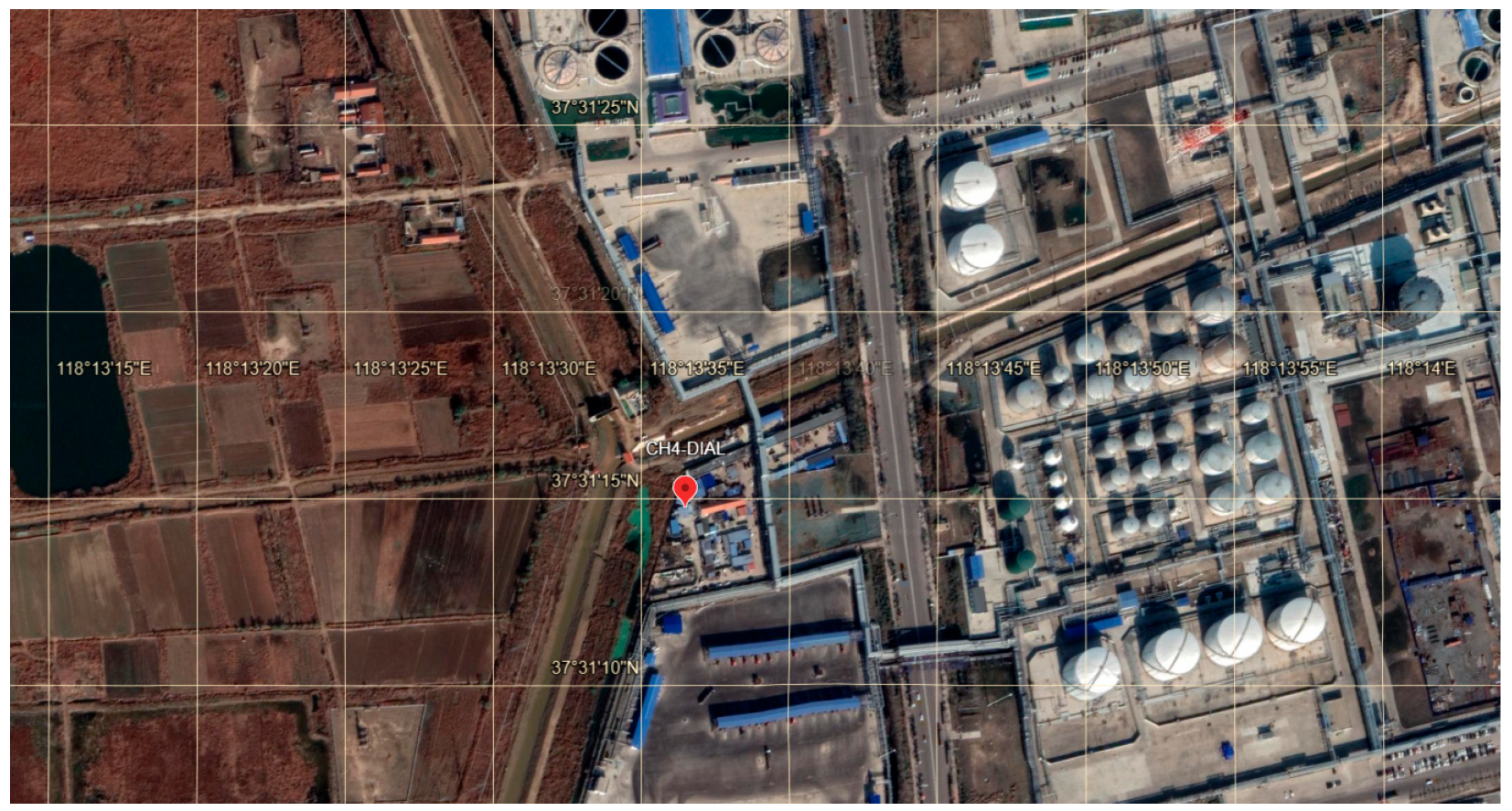
2.1. Study Area

Dongying City is the central city in the Yellow River Delta region, with a geographical location spanning N 36°55′ to 38°10′, E 118°07′ to 119°15′. Dongying City belongs to a typical temperate continental monsoon climate with distinct four seasons. The terrain of Dongying City is flat, with plains as the main terrain. Its eastern and northern parts are adjacent to the Bohai Sea, with many rivers and abundant marine resources. A large number of salt and aquaculture farms are distributed in coastal areas, and natural resources such as oil and gas are abundant. The CH₄-DIAL was placed at the location shown in Figure 1. There is a large amount of farmland and vegetation distributed to the west of the observation site. The east side has multitudinous buildings, being a densely populated area.

2.2. CH₄-DIAL

The Lidar signal data used in this study were obtained from a self-developed DIAL system. It consists of two main parts: a laser emitting unit and a signal receiving unit. The seed laser’s on-/off-line wavelengths are generated by two 1.65 μm continuous lasers, respectively, and the two wavelengths are quickly switched using fiber switches. Due to the continuous sampling capability of the laser source, the CH₄ saturated absorption spectrum is used to lock the laser frequency at the specified frequency, which has high stability. The pump laser is emitted by a Nd: YAG laser that outputs a narrow linewidth of 1064nm infrared. The switching of on-/off-line wavelength lasers is completed in the form of seed laser timing switching. The signal receiving unit mainly consists of a telescope, ultra-narrow-band filters, etc. Background light noise is suppressed through an ultra-narrow-band filter, thereby improving the daytime detection capability of the Lidar system. The hardware parameters are shown in

Table 1. The parameters for CH₄-DIAL.

Paramter	Value
On-line (cm−1)	6076.984
Off-line (cm−1)	6077.653
Pulse energy (mJ)	21
Repetition rate (Hz)	20
Pulse length (ns)	10
Linewidth (MHz)	200
Telescope Diameter (mm)	400
Beam divergence (mrad)	0.1
Overall optical efficient	52.6
Quantum efficiency (%)	85

. The CH₄-DIAL system was deployed at the observation site to measure data for the entire year of 2023. In addition, in order to validate the proposed method through real examples, an Aircore system based on unmanned aerial vehicles was utilized. The system collects air samples from different heights and analyzes them using a high-precision cavity ring-down spectrometer (Picaro G2401, Picarro, Inc. Santa Clara, CA, USA). Three cases were measured on 12 April 2023 at 20:00, 16 July 2023 at 21:00, and 6 December 2023 at 17:00, respectively.

2.3. Auxiliary Data

Due to the direct impact of atmospheric temperature and pressure on the calculation accuracy of the absorption cross-section, the uncertainty of atmospheric factors can bring errors to the retrieval of range-resolved concentrations. Therefore, the Lidar system was equipped with an auxiliary microwave radiometer to obtain real-time temperature and pressure data to improve accuracy.

3. Methods

3.1. DIAL Principle

The DIAL emits two laser beams of different wavelengths. One is located at the absorption peak of the target gas molecule, which is called the on-line wavelength and can strongly absorb the target gas. The other, located outside the absorption peak of the target gas, is called the off-line wavelength, which has very little absorption effect on the gas. The wavelengths of these two lasers are close enough that their atmospheric scattering characteristics are similar. Therefore, the differences in atmospheric backscattering, aerosol and atmospheric molecular extinction between the on-line and off-line lasers can be ignored. This ensures that any measured difference in the returned signals is due to the absorption of the target gas rather than the influence of other factors. CH₄-DIAL measures the degree of difference between the two laser signals to calculate the concentration information of methane gas at different distances. The foundation of DIAL technology is the backscatter Lidar equation:

$${\mathrm{E}}_{\mathsf{\lambda }}\left(\mathrm{r}\right)={\displaystyle \frac{{\mathsf{\xi }}_{\mathsf{\lambda }}·{\mathrm{E}}_{0,\mathsf{\lambda }}·\mathrm{A}·{\mathsf{\beta }}_{\mathrm{i}}\left(\mathrm{r}\right)·\mathrm{c}·\mathsf{\eta }\left(\mathrm{r}\right)}{2·{\mathrm{r}}^2}}·\exp \left(-2·{{\displaystyle \int }}_0^{\mathrm{r}}\left({\mathsf{\alpha }}_{\mathsf{\lambda }}\left(\mathrm{r}\right){+\mathrm{N}}_{\mathrm{g}}·{\mathsf{\sigma }}_{\mathrm{g}}\left(\mathsf{\lambda }\right)\right)\right)$$

(1)

where r is the detection range (distance from target to receiver); ${\mathrm{E}}_{\mathsf{\lambda }}$ is the received energy of range r; ${\mathsf{\xi }}_{\mathsf{\lambda }}$ denotes the total instrument efficiency for wavenumber λ; ${\mathrm{E}}_{0,\mathsf{\lambda }}$ is the output energy of a single laser pulse; A refers to the receiver area of the telescope; β_i(r) is the backscatter coefficient of the atmosphere; c is the speed of light; η(r) denotes the overlap function; α_λ(r) refers to the extinction coefficient of the atmosphere; N_g represents the number density of a trace gas; ${\mathsf{\sigma }}_{\mathrm{g}}\left(\mathsf{\lambda }\right)$ indicates the absorption cross section of the trace gas.

The laser pulses emitted by online and offline wavelengths indicate that the signal received by the DIAL can be expressed as differential absorption optical depth (DAOD). This represents the optical thickness of CH₄, which is related to the number density of CH₄, detection range, and position of the online and offline wavenumbers, which can be calculated by:

$$\mathrm{DAOD}=\ln {\displaystyle \frac{{\mathrm{E}}_{{\mathsf{\lambda }}_{\mathrm{off}}}\left({\mathrm{r}}_{\mathrm{top}}\right)·{\mathrm{E}}_{{\mathsf{\lambda }}_{\mathrm{on}}}\left({\mathrm{r}}_{\mathrm{bottom}}\right)}{{\mathrm{E}}_{{\mathsf{\lambda }}_{\mathrm{on}}}\left({\mathrm{r}}_{\mathrm{top}}\right)·{\mathrm{E}}_{{\mathsf{\lambda }}_{\mathrm{off}}}\left({\mathrm{r}}_{\mathrm{bottom}}\right)}}$$

(2)

where ${\mathrm{r}}_{\mathrm{top}}$ and ${\mathrm{r}}_{\mathrm{bottom}}$ denote the beginning and end of the integration interval, and ${\mathrm{E}}_{{\mathsf{\lambda }}_{\mathrm{off}}}\left(\mathrm{r}\right)$ and ${\mathrm{E}}_{{\mathsf{\lambda }}_{\mathrm{on}}}\left(\mathrm{r}\right)$ represent the received energy of ${\mathsf{\lambda }}_{\mathrm{off}}$ and ${\mathsf{\lambda }}_{\mathrm{on}}$ at range r.

According to DAOD, the number density of CH₄ at different distances can be calculated by:

$${\mathrm{N}}_{{\mathrm{CH}}_4}\left(\mathrm{r}\right)={\displaystyle \frac{\mathrm{DAOD}\left(\mathrm{r}\right)}{2\left({\mathrm{r}}_{\mathrm{top}}{-\mathrm{r}}_{\mathrm{bottom}}\right)·\left[{\mathsf{\sigma }}_{{\mathsf{\lambda }}_{\mathrm{on}}}\left(\mathrm{r}\right)-\left(\mathrm{r}\right)\right]}}$$

(3)

where ${\mathsf{\sigma }}_{{\mathsf{\lambda }}_{\mathrm{on}}}\left(\mathrm{r}\right)$ and ${\mathsf{\sigma }}_{{\mathsf{\lambda }}_{\mathrm{off}}}\left(\mathrm{r}\right)$ denote the CH₄ absorption cross sections of ${\mathsf{\lambda }}_{\mathrm{on}}$ and ${\mathsf{\lambda }}_{\mathrm{off}}$ at the range of $\mathrm{r}$. The CH₄ absorption cross section is closely related to temperature, pressure and height. This indicates that the detection results of CH₄ are closely related to environmental parameters, especially temperature and pressure. The spectral data used in this article are from the HITRAN database.

The number density of CH₄ is further converted into a dry-air mixing ratio (XCH₄) in parts per billion (ppb) by:

$${\mathrm{XCH}}_4\left(\mathrm{r}\right)={\displaystyle \frac{{\mathrm{N}}_{{\mathrm{CH}}_4}\left(\mathrm{r}\right)}{{\mathrm{N}}_{\mathrm{air}}\left(\mathrm{r}\right)}}$$

(4)

where ${\mathrm{N}}_{{\mathrm{CH}}_4}\left(\mathrm{r}\right)$ denotes the number density of CH₄ at the range of r; ${\mathrm{N}}_{\mathrm{air}}\left(\mathrm{r}\right)$ represents the number density of air molecule at the range of r.

3.2. Cubic Smoothing Spline Fitting

Traditional methods use various signal denoising methods to approach the real data as closely as possible, and then directly calculate profile information based on the Lidar equation. The denoising methods mainly revolve around low-pass filtering, with commonly used methods including multi-pulse averaging, Fourier Transform, Empirical Mode Decomposition and Wavelet Transform. However, the principle of DIAL is based on the Mie scattering of aerosols, which mainly exist in the troposphere. The concentration of aerosols decreases with increasing altitude, and there are fewer aerosol particles above the atmospheric boundary layer height. Therefore, as height increases, the signal strength gradually weakens and the SNR gradually decreases. This can be verified in an example of the relationship between signal-to-noise ratio and detection height measured by the CH₄-DIAL, as shown in Figure 2. There are two main reasons for such a phenomenon: (1) emitting lasers will be absorbed by CH₄ molecules in the atmosphere; (2) aerosol scattering on the detection path will attenuate the energy of the pulsed laser, and the longer the laser transmission distance, the stronger the attenuation effect. Within the height of the boundary layer, Lidar signals typically have high accuracy and rich redundant observations. However, raw Lidar signals at high altitudes exhibit significant fluctuations, leading to poor accuracy in the retrieval of CH₄ concentration. Therefore, traditional retrieval methods are not suitable for dealing with the problem of different and large fluctuations of signals at different heights. Fortunately, applying cubic smoothing splines to single original signals can ensure that the signal curves have minimum nonlinear error throughout the entire detection range. This optimization of the overall signal can ensure the overall accuracy and stability of the entire profile.

Cubic smoothing splines are developed on the basis of cubic spline interpolation. Cubic spline interpolation is conducted by dividing the sample into multiple intervals and using a cubic function for interpolation on each interval. The interpolation function must meet the following requirements:

• The left endpoint function value of each interpolation function is equal to its left endpoint sample value.
• Except for the first and last endpoints, the left and right first derivatives of the middle endpoints are equal.
• Except for the first and last endpoints, the left and right second derivatives of the middle endpoints are equal.

Based on the above requirements, the interpolation function for each interval can be derived. However, due to the possible presence of noise at the sample points, cubic spline interpolation requires the interpolation function to pass through all sample points. Noise may cause drastic fluctuations in the calculated overall interpolation function, resulting in unsatisfactory results. Cubic spline smoothing does not require the function to pass through all sample points, which can avoid this drawback. A cubic smoothing spline is an optimization of the smoothing spline function value and sample value using the least squares method, with constraints on the second derivative of the smoothing spline functions added. If the absolute value of the second derivative within the interval of the smoothing spline function is large, the curvature of the spline function will be high. The overall smoothing spline function will be very curved, presenting a shape with violent fluctuations. In this case, the smoothing spline function exhibits an unnatural overfitting state and is greatly affected by noise. The objective function of the cubic smoothing spline is as follows:

$${{\displaystyle \sum }}_{\mathrm{i}=1}^{\mathrm{n}}{\left({\mathrm{y}}_{\mathrm{i}}-\mathrm{g}\left({\mathrm{u}}_{\mathrm{i}}\right)\right)}^2+\mathsf{\lambda }\int {\mathrm{g}}^{″}{\left(\mathrm{v}\right)}^2\mathrm{dv}$$

(5)

where ${\mathrm{y}}_{\mathrm{i}}$ is the value of the sample-dependent variables; g represents the cubic smoothing spline function; ${\mathrm{u}}_{\mathrm{i}}$ denotes the value of the sample independent variables; λ refers to the smoothing coefficient. The first term in the function is the least squares form of the sample values and the spline function values. The second term is the penalty term for the second derivative of the spline function.

It should be noted that misalignment between the laser beam and its receiving optical axis, as well as asymmetric laser intensity distribution, will cause the overlap factor. Furthermore, in DIAL, the detection results are based on differential calculations and are highly sensitive to the strength of the on-line and off-line received signals. However, relative consistency of the on-line and off-line signals cannot be guaranteed in overlapping areas. Therefore, in order to avoid differential calculation errors caused by the overlap factor, the starting height of retrieval is set to 300 m.

3.3. Statistical Method

The accuracy of the CH₄ profile concentration is evaluated using the correlation coefficient (R), mean error (ME), mean absolute error (MAE) and standard deviation (STD). R represents the degree of linear correlation between variables, calculated as follows:

$$\mathrm{R}={\displaystyle \frac{{{\displaystyle \sum }}_{\mathrm{i}=1}^{\mathrm{n}}\left({\mathrm{x}}_{\mathrm{i}}-\overline{\mathrm{x}}\right)\left({\mathrm{y}}_{\mathrm{i}}-\overline{\mathrm{y}}\right)}{\sqrt{{{\displaystyle \sum }}_{\mathrm{i}=1}^{\mathrm{n}}{\left({\mathrm{x}}_{\mathrm{i}}-\overline{\mathrm{x}}\right)}^2}\sqrt{{{\displaystyle \sum }}_{\mathrm{i}=1}^{\mathrm{n}}{\left({\mathrm{y}}_{\mathrm{i}}-\overline{\mathrm{y}}\right)}^2}}}$$

(6)

where x and y represent the two sets of samples, respectively;$\overline{\mathrm{x}}$ and $\overline{\mathrm{y}}$ denote the mean values of these two sets of samples, respectively.

Both ME and MAE represent the error between the retrieved value and the true value:

$$\mathrm{ME}={\displaystyle \frac{1}{\mathrm{n}}}{{\displaystyle \sum }}_{\mathrm{i}=1}^{\mathrm{n}}\left({\mathrm{y}}_{\mathrm{i}}-\widehat{{\mathrm{y}}_{\mathrm{i}}}\right)$$

(7)

$$\mathrm{MAE}={\displaystyle \frac{1}{\mathrm{n}}}{{\displaystyle \sum }}_{\mathrm{i}=1}^{\mathrm{n}}\left|\left({\mathrm{y}}_{\mathrm{i}}-\widehat{{\mathrm{y}}_{\mathrm{i}}}\right)\right|$$

(8)

where ${\mathrm{y}}_{\mathrm{i}}$ and $\widehat{{\mathrm{y}}_{\mathrm{i}}}$ denote the true value and estimated value, respectively.

The STD reflects the degree of dispersion of a set of data, which is an important indicator of accuracy. It can be calculated by:

$$\mathrm{STD}=\sqrt{{\displaystyle \frac{{{\displaystyle \sum }}_{\mathrm{i}=1}^{\mathrm{n}}{\left({\mathrm{x}}_{\mathrm{i}}-\overline{\mathrm{x}}\right)}^2}{\mathrm{n}}}}$$

(9)

4. Results and Discussion

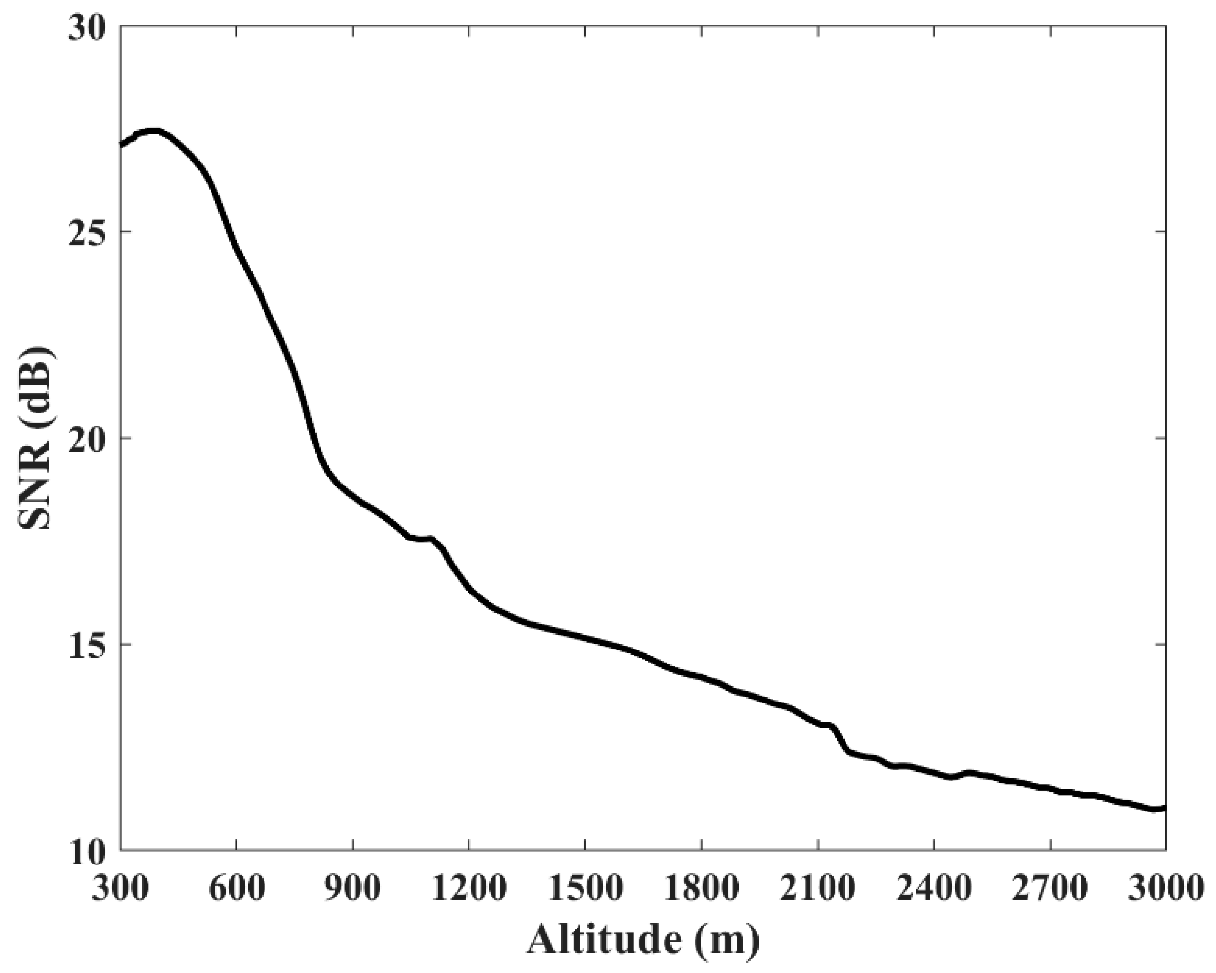
4.1. Simulations

In order to verify the superiority of the proposed method, simulation comparisons were conducted between the traditional method, Chebyshev fitting [32], and cubic smoothing spline fitting. In these simulations, we set the simulation range to an altitude of 300–1875 m (assumed boundary layer height) with a layer interval of 7.5 m. The simulated CH₄ concentration ranged from 1400 ppb to 1800 ppb and the integration time was 10 min. Ten simulations were conducted in total, and the average was taken as the simulation result. The vertical profiles of temperature and pressure are given according to the American standard atmospheric model [34]. Based on the simulated Lidar signal and the vertical profiles of temperature and pressure, three methods were used to retrieve the CH₄ concentration profile. The retrieved results were compared with the simulated CH₄ concentration profile and the performance of the three methods was evaluated based on statistical indicators.

Figure 3a compares the MEs of CH₄ concentration profiles obtained by different methods. The ME of the traditional method is the largest, ranging from 0.18 to 22.19 ppb, which indicates that the accuracy of CH₄ profile concentration inversion using the traditional method is the lowest. Moreover, the ME of the traditional method has significant fluctuations. It proves that the traditional method is not suitable for dealing with the problem of large fluctuations in signals at high altitudes. The results of Chebyshev fitting are shown by the red dashed line in Figure 3a. The maximum ME is only 1.40 ppb, which is one order of magnitude smaller than the traditional method. Cubic smoothing spline fitting shows the best performance, with its ME being lower than the other two methods at almost all heights. Compared with the traditional method, cubic smoothing spline fitting can reduce the ME of the whole CH₄ concentration profile by 85.54%.

Figure 3b shows the MAE of the CH₄ concentration profile calculated using different methods. It can be seen that, except for below 400 m, the MAE of the cubic smoothing spline fitting results is smaller than that of the other two methods in each layer. Specifically, within the initial range of 300 m–420 m, the ME and MAE of the CH₄ concentration profile calculated using Chebyshev fitting and cubic smoothing spline fitting are both slightly greater than those calculated using the traditional method. This is because Chebyshev fitting and cubic smoothing spline fitting not only focus on accuracy at a certain height of the profile, but also ensure that the overall fitting error of the profile is minimized. Therefore, noise at high altitudes may have an impact on signals with high SNR at low altitudes, resulting in slight errors. Nevertheless, there is not much difference in accuracy among the three methods at low altitude, while the accuracy of the two fitting methods is much higher than that of the traditional method at high altitudes. Overall, it can still be considered that Chebyshev fitting and cubic smoothing spline fitting perform better than the traditional method. Compared with traditional methods, the maximum reduction in the MAE of the CH₄ concentration profile calculated by them was 96.59 ppb and 107.33 ppb, respectively.

Figure 3c shows the difference between the STD of the traditional method and Chebyshev fitting results and the STD of the cubic smoothing spline fitting results at different altitudes. It can be seen that the STD of the CH₄ concentration profile obtained by cubic smoothing spline fitting is smaller than that of the other two methods at all heights. The STD of the CH₄ concentration retrieved using cubic smoothing spline fitting is 3.59 ppb–90.29 ppb (0.01 ppb–6.75 ppb) smaller than the traditional method (Chebyshev method). This indicates that the stability of cubic smoothing spline retrieval is better than that of the other two methods and therefore has higher robustness. In summary, the proposed cubic smoothing spline fitting method has the best accuracy and precision in retrieving CH₄ concentration profiles.

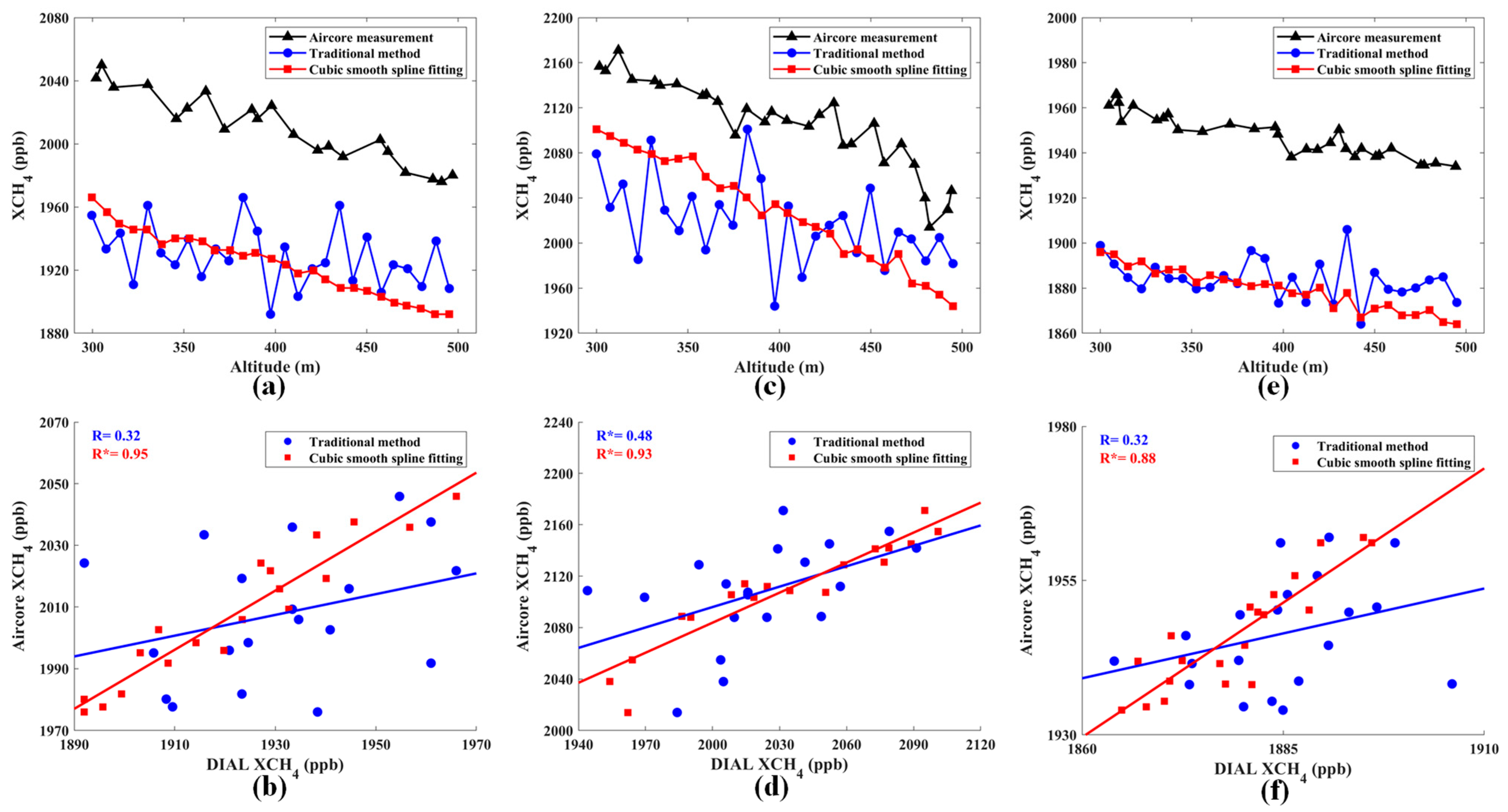
4.2. Case Verification

Three case verifications were carried out to demonstrate the advantages of the proposed method. A drone-based Aircore system was developed to collect real CH₄ concentration profile data. Then, the air samples acquired by the active Aircore were analyzed using a high-precision Cavity ring-down spectrometer (Picaro G2401). It should be noted that considering the overlap factor of DIAL and the drone flight altitude setting, the case data collection altitude range was set to 300–500 m. Temporal and spatial matching of these two instruments was conducted to ensure the accuracy of the comparison. During the measurement process, good matching was acquired by measuring simultaneously and at the same location. The concentration data collected from these three cases and the CH₄ concentration profiles retrieved using two methods based on DIAL data are shown in Figure 4. Figure 4a,c,e represent the CH₄ concentration profiles obtained from the three cases of in-situ measurements and two DIAL retrieval methods. It can be seen that the CH₄ concentration profile obtained by the traditional method (blue circles) exhibits significant fluctuations. The stability of the CH₄ concentration profiles obtained by cubic smoothing spline fitting is excellent, and their trend is consistent with the observation results collected by Aircore. In order to quantitatively compare the accuracy of the two retrieval methods, the average of all Aircore observed concentrations in each layer was calculated. This yielded a one-to-one correspondence between DIAL concentration and Aiecore observations, which is plotted in Figure 4b,d,f. It can be seen that the CH₄ concentration calculated by cubic smoothing spline fitting is more consistent with the concentrations observed by Aircore compared to the traditional method. The cubic smoothing spline fitting results have higher R with all values above 0.88, and all three cases pass the significance test. In contrast, the R of the traditional method only ranges from 0.32 to 0.48, and two cases do not pass the significance test. In summary, the CH₄ concentration profile retrieved by cubic smoothing spline fitting has better accuracy and reliability than the traditional method. Additionally, it should be noted that the CH₄ concentration calculated from DIAL is generally lower than the actual measurement by Aircore, with a difference of about 50 ppb–80 ppb. Firstly, the measurement time for these two concentration results is different. In-situ measurement is instantaneous, while DIAL measurements are the result of ten-minute integration. Secondly, environmental factors such as the propeller and airflow of drones may have a notable impact on the Aircore measurements. In addition, issues with instrument calibration and spectral data can also lead to this fixed bias.

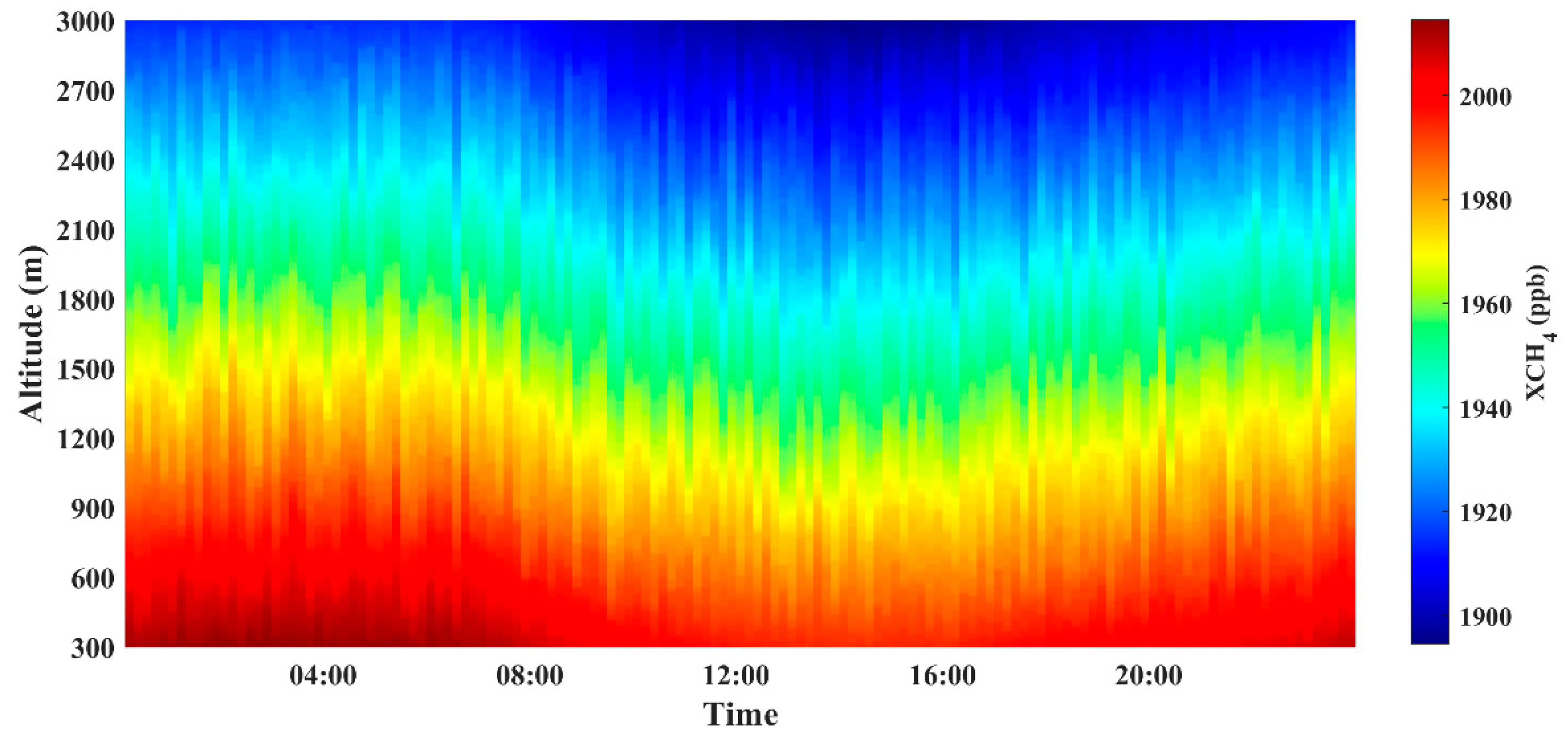
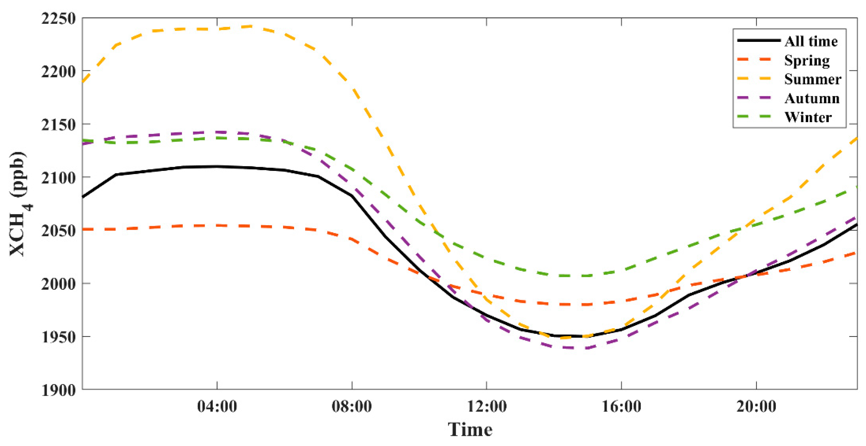
4.3. Diurnal Variation

The changes in methane concentration at the observation site were explored using long-term DIAL data. The variation in CH₄ concentration profile during one day was plotted in Figure 5. The concentration of CH₄ varies between 1897 ppb and 2024 ppb in a day with a clear diurnal trend, which is similar to [34,35]. It gradually increases from midnight until it reaches its peak around 4:00, then gradually decreases to a valley around 16:00, and increases again at night. The diurnal variation in CH₄ concentration is mainly influenced by emissions from CH₄ sources, the impact of atmospheric OH radical concentration on CH₄ sinks, and meteorological factors such as boundary layer height [36,37,38].

To characterize the daily variation in CH₄ concentration over a long period of time, we integrated data at the vertical altitude to obtain the average CH₄ concentration. The average hourly CH₄ concentration for each season and year was averaged to investigate diurnal variation in CH₄ concentration (Figure 6). The average CH₄ concentration in different seasons and throughout the year exhibits an obvious diurnal variation trend, being low during daytime and high during nighttime. The pattern is similar to existing research results [39,40,41]. The CH₄ concentration increases to its peak at 4:00, then gradually decreases to the lowest value at 15:00 and gradually increases again after sunset, because the stable boundary layer structure at night is not conducive to the diffusion of CH₄, and thus the concentration gradually accumulates. At the same time, the reduction in OH radicals in the nighttime atmosphere results in a smaller consumption of methane. The combined effect of these two factors causes the atmospheric CH₄ concentration to accumulate and reach its peak around 4:00. After sunrise, solar radiation increases and the concentration of OH radicals in the atmosphere increases, which enhances the consumption of CH₄. In addition, as the temperature increases, convective activity in the boundary layer intensifies, and the height of the boundary layer gradually increases. A strong diffusion effect leads to a gradual decrease in CH₄ concentration, reaching a valley around 15:00. The diurnal variation pattern is roughly the same throughout the year and each season with only slight differences in the magnitude of the variation. The maximum variation in CH₄ concentration during summer is about 294 ppb. The diurnal variation in CH₄ concentration in autumn is also relatively strong, with an amplitude of about 203 ppb, and the amplitude in winter is 130 ppb. The diurnal variation range of CH₄ concentration in spring is the smallest, about 75 ppb. Over the whole year, the fluctuation range of the average CH₄ concentration is approximately 160.84. From an emissions perspective, high temperatures in summer result in higher biogenic methane emissions near the ground, leading to higher overall CH₄ concentrations compared to other seasons.

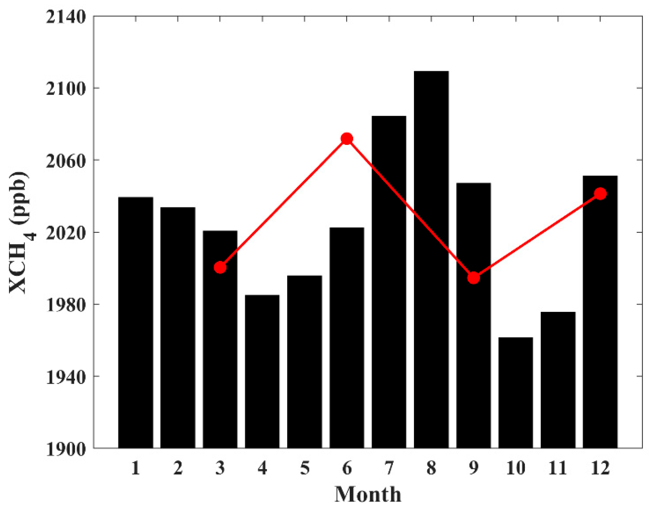
4.4. Monthly and Seasonal Variation

After a one-year observation by DIAL, the monthly average CH₄ concentration at the observation site was explored. The results are shown in Figure 7. The black bars represent the average CH₄ concentration in different months, and the red lines represent the average CH₄ concentration in different seasons. March, April, and May are designated as spring, June, July, and August are designated as summer, September, October, and November are designated as autumn, and December, January, and February are designated as winter. From a monthly perspective, August has the highest average CH₄ concentration with about 2109 ppb, while October has the lowest average CH₄ concentration with approximately 1961 ppb. The annual amplitude of monthly average CH₄ concentration is 148 ppb. The annual CH₄ concentration exhibits a significant W-shaped variation trend. From a seasonal perspective, the average CH₄ concentration is highest in summer (2072 ppb), followed by winter (2041 ppb), and lowest in autumn (1995 ppb). This is because summer has high temperatures and abundant rainfall, which is the period when vegetation and other biological sources discharge most vigorously. Moreover, high temperature and humidity conditions are more conducive to the anaerobic decomposition of ruminants and waste treatment processes, resulting in more methane emissions. At the same time, strong methane emissions from farmland in summer also contribute to the atmospheric CH₄ concentration to a certain extent. In winter, the increase in CH₄ concentration may be related to heating in the north. Widespread heating leads to a massive increase in methane emissions. Generally, the trend is similar to [42,43], but there may be slight differences. These difference are due to a combination of factors such as the environment, climate, and anthropogenic emissions at the measurement site.

5. Conclusions

A new method based on CH₄-DIAL is proposed to improve the accuracy of CH₄ concentration profile retrieval. This method utilizes cubic smoothing spline fitting to fully utilize high SNR signals and redundant observations within the boundary layer, ensuring that the CH₄ concentration within the entire detection range has the minimum nonlinear error.

By simulating Lidar signals, the proposed method is compared with traditional methods through simulations. The results indicate that the performance of cubic smoothing splines is better than the traditional method. Compared with the traditional method, cubic smoothing spline fitting can reduce the ME of the entire CH₄ concentration profile by 85.54%. In addition, the proposed method is also superior to Chebyshev fitting. Its STD is 0.01 ppb–6.75 ppb smaller than that of Chebyshev fitting. Three cases prove that the CH₄ concentration obtained by cubic smoothing spline fitting has a more consistent trend relative to in-situ observed concentration compared to the traditional method. It has higher correlation coefficients, all above 0.88. Compared to the traditional method, the proposed method has smaller volatility and better stability. Finally, using long-term DIAL measurements, the diurnal and monthly variations of the average CH₄ concentration were investigated at the observation site. The average concentration of CH₄ in each season and throughout the year shows a clear diurnal trend. Among them, the diurnal variation amplitude of CH₄ concentration in summer is the largest, about 294 ppb. From a seasonal perspective, the average CH₄ concentration is highest in summer (2072 ppb) and lowest in autumn (1995 ppb).

However, there is a deviation between in-situ CH₄ measurements and the CH₄ concentrations retrieved from DIAL data, which may be caused by different measurement mechanisms or environmental influences (such as drone propellers). In-situ measurements are instantaneous, while DIAL measures the time-averaged signal. In addition, the retrieval results at high altitudes have not yet been validated. In the future, attention will also be paid to optimizing accuracy within the entire detection range while avoiding the influence of noise at high altitudes on signals at low altitudes.

References

1. Rogelj, J.; den Elzen, M.; Höhne, N.; Fransen, T.; Fekete, H.; Winkler, H.; Schaeffer, R.; Sha, F.; Riahi, K.; Meinshausen, M. Paris Agreement Climate Proposals Need a Boost to Keep Warming Well below 2 °C. Nature 2016, 534, 631–639. [Google Scholar] [CrossRef] [PubMed]
2. Tian, H.; Lu, C.; Ciais, P.; Michalak, A.M.; Canadell, J.G.; Saikawa, E.; Huntzinger, D.N.; Gurney, K.R.; Sitch, S.; Zhang, B.; et al. The Terrestrial Biosphere as a Net Source of Greenhouse Gases to the Atmosphere. Nature 2016, 531, 225–228. [Google Scholar] [CrossRef] [PubMed]
3. Dean, J.F.; Middelburg, J.J.; Röckmann, T.; Aerts, R.; Blauw, L.G.; Egger, M.; Jetten, M.S.M.; de Jong, A.E.E.; Meisel, O.H.; Rasigraf, O.; et al. Methane Feedbacks to the Global Climate System in a Warmer World. Rev. Geophys. 2018, 56, 207–250. [Google Scholar] [CrossRef]
4. Hasegawa, T.; Sakurai, G.; Fujimori, S.; Takahashi, K.; Hijioka, Y.; Masui, T. Extreme Climate Events Increase Risk of Global Food Insecurity and Adaptation Needs. Nat. Food 2021, 2, 587–595. [Google Scholar] [CrossRef] [PubMed]
5. Zittis, G.; Almazroui, M.; Alpert, P.; Ciais, P.; Cramer, W.; Dahdal, Y.; Fnais, M.; Francis, D.; Hadjinicolaou, P.; Howari, F.; et al. Climate Change and Weather Extremes in the Eastern Mediterranean and Middle East. Rev. Geophys. 2022, 60, e2021RG000762. [Google Scholar] [CrossRef]
6. Cai, W.; Wang, G.; Dewitte, B.; Wu, L.; Santoso, A.; Takahashi, K.; Yang, Y.; Carreric, A.; McPhaden, M.J. Increased Variability of Eastern Pacific El Nino under Greenhouse Warming. Nature 2018, 564, 201–206. [Google Scholar] [CrossRef] [PubMed]
7. Jones, M.W.; Peters, G.P.; Gasser, T.; Andrew, R.M.; Schwingshackl, C.; Guetschow, J.; Houghton, R.A.; Friedlingstein, P.; Pongratz, J.; Le Quere, C. National Contributions to Climate Change Due to Historical Emissions of Carbon Dioxide, Methane, and Nitrous Oxide since 1850. Sci. Data 2023, 10, 155. [Google Scholar] [CrossRef] [PubMed]
8. Arndt, C.; Hristov, A.N.; Price, W.J.; McClelland, S.C.; Pelaez, A.M.; Cueva, S.F.; Oh, J.; Dijkstra, J.; Bannink, A.; Bayat, A.R.; et al. Full Adoption of the Most Effective Strategies to Mitigate Methane Emissions by Ruminants Can Help Meet the 1.5 °C Target by 2030 but Not 2050. Proc. Natl. Acad. Sci. USA 2022, 119, e2111294119. [Google Scholar] [CrossRef] [PubMed]
9. Intergovernmental Panel on Climate Change (IPCC) (Ed.) Anthropogenic and Natural Radiative Forcing. In Climate Change 2013—The Physical Science Basis: Working Group I Contribution to the Fifth Assessment Report of the Intergovernmental Panel on Climate Change; Cambridge University Press: Cambridge, UK, 2014; pp. 659–740. ISBN 978-1-107-05799-9. [Google Scholar]
10. World Meteorological Organization. WMO Greenhouse Gas Bulletin No. 19; The state of greenhouse gases in the atmosphere based on global observations through 2022; World Meteorological Organization: Geneva, Switzerland, 2023. [Google Scholar]
11. Ehhalt, D.H.; Schmidt, U. Sources and Sinks of Atmospheric Methane. PAGEOPH 1978, 116, 452–464. [Google Scholar] [CrossRef]
12. Turner, A.J.; Frankenberg, C.; Kort, E.A. Interpreting Contemporary Trends in Atmospheric Methane. Proc. Natl. Acad. Sci. USA 2019, 116, 2805–2813. [Google Scholar] [CrossRef]
13. Prather, M.J.; Holmes, C.D.; Hsu, J. Reactive Greenhouse Gas Scenarios: Systematic Exploration of Uncertainties and the Role of Atmospheric Chemistry. Geophys. Res. Lett. 2012, 39. [Google Scholar] [CrossRef]
14. Jacob, D.J.; Turner, A.J.; Maasakkers, J.D.; Sheng, J.; Sun, K.; Liu, X.; Chance, K.; Aben, I.; McKeever, J.; Frankenberg, C. Satellite Observations of Atmospheric Methane and Their Value for Quantifying Methane Emissions. Atmos. Chem. Phys. 2016, 16, 14371–14396. [Google Scholar] [CrossRef]
15. Messerschmidt, J.; Geibel, M.C.; Blumenstock, T.; Chen, H.; Deutscher, N.M.; Engel, A.; Feist, D.G.; Gerbig, C.; Gisi, M.; Hase, F.; et al. Calibration of TCCON Column-Averaged CO2: The First Aircraft Campaign over European TCCON Sites. Atmos. Chem. Phys. 2011, 11, 10765–10777. [Google Scholar] [CrossRef]
16. Laughner, J.L.; Toon, G.C.; Mendonca, J.; Petri, C.; Roche, S.; Wunch, D.; Blavier, J.-F.; Griffith, D.W.T.; Heikkinen, P.; Keeling, R.F.; et al. The Total Carbon Column Observing Network’s GGG2020 Data Version. Earth Syst. Sci. Data 2024, 16, 2197–2260. [Google Scholar] [CrossRef]
17. Jacob, D.J.; Varon, D.J.; Cusworth, D.H.; Dennison, P.E.; Frankenberg, C.; Gautam, R.; Guanter, L.; Kelley, J.; McKeever, J.; Ott, L.E.; et al. Quantifying Methane Emissions from the Global Scale down to Point Sources Using Satellite Observations of Atmospheric Methane. Atmos. Chem. Phys. 2022, 22, 9617–9646. [Google Scholar] [CrossRef]
18. Kiemle, C.; Ehret, G.; Amediek, A.; Fix, A.; Quatrevalet, M.; Wirth, M. Potential of Spaceborne Lidar Measurements of Carbon Dioxide and Methane Emissions from Strong Point Sources. Remote Sens. 2017, 9, 1137. [Google Scholar] [CrossRef]
19. Liang, A.; Gong, W.; Han, G.; Xiang, C. Comparison of Satellite-Observed XCO2 from GOSAT, OCO-2, and Ground-Based TCCON. Remote Sens. 2017, 9, 1033. [Google Scholar] [CrossRef]
20. Riris, H.; Numata, K.; Wu, S.; Gonzalez, B.; Rodriguez, M.; Kawa, S.; Mao, J. Methane Measurements from Space: Technical Challenges and Solutions. In Laser Radar Technology and Applications XXII, 5 May 2017; SPIE: Bellingham, WT, USA, 2017; Volume 10191, pp. 17–26. [Google Scholar]
21. Kiemle, C.; Kawa, S.R.; Quatrevalet, M.; Browell, E.V. Performance Simulations for a Spaceborne Methane Lidar Mission. J. Geophys. Res. Atmos. 2014, 119, 4365–4379. [Google Scholar] [CrossRef]
22. Weaver, C.; Kiemle, C.; Kawa, S.R.; Aalto, T.; Necki, J.; Steinbacher, M.; Arduini, J.; Apadula, F.; Berkhout, H.; Hatakka, J. Retrieval of Methane Source Strengths in Europe Using a Simple Modeling Approach to Assess the Potential of Spaceborne Lidar Observations. Atmos. Chem. Phys. 2014, 14, 2625–2637. [Google Scholar] [CrossRef]
23. Zhang, X.; Zhang, M.; Bu, L.; Fan, Z.; Mubarak, A. Simulation and Error Analysis of Methane Detection Globally Using Spaceborne IPDA Lidar. Remote Sens. 2023, 15, 3239. [Google Scholar] [CrossRef]
24. Tellier, Y.; Pierangelo, C.; Wirth, M.; Gibert, F.; Marnas, F. Averaging Bias Correction for the Future Space-Borne Methane IPDA Lidar Mission MERLIN. Atmos. Meas. Tech. 2018, 11, 5865–5884. [Google Scholar] [CrossRef]
25. Han, G.; Xu, H.; Gong, W.; Liu, J.; Du, J.; Ma, X.; Liang, A. Feasibility Study on Measuring Atmospheric CO2 in Urban Areas Using Spaceborne CO2-IPDA LIDAR. Remote Sens. 2018, 10, 985. [Google Scholar] [CrossRef]
26. Refaat, T.F.; Ismail, S.; Nehrir, A.R.; Hair, J.W.; Crawford, J.H.; Leifer, I.; Shuman, T. Performance Evaluation of a 1.6-Μm Methane DIAL System from Ground, Aircraft and UAV Platforms. Opt. Express 2013, 21, 30415–30432. [Google Scholar] [CrossRef] [PubMed]
27. Hrad, M.; Huber-Humer, M.; Reinelt, T.; Spangl, B.; Flandorfer, C.; Innocenti, F.; Yngvesson, J.; Fredenslund, A.; Scheutz, C. Determination of Methane Emissions from Biogas Plants, Using Different Quantification Methods. Agric. For. Meteorol. 2022, 326, 109179. [Google Scholar] [CrossRef]
28. Ma, X.; Shi, T.; Xu, H.; He, B.; Qiu, R.; Han, G.; Gong, W. On-Line Wavenumber Optimization for a Ground-Based CH4-DIAL. J. Quant. Spectrosc. Radiat. Transf. 2019, 229, 106–119. [Google Scholar] [CrossRef]
29. Philip, S.; Johnson, M.S.; Potter, C.; Genovesse, V.; Baker, D.F.; Haynes, K.D.; Henze, D.K.; Liu, J.; Poulter, B. Prior Biosphere Model Impact on Global Terrestrial CO2 Fluxes Estimated from OCO-2 Retrievals. Atmos. Chem. Phys. 2019, 19, 13267–13287. [Google Scholar] [CrossRef]
30. Agusti-Panareda, A.; Massart, S.; Chevallier, F.; Boussetta, S.; Balsamo, G.; Beljaars, A.; Ciais, P.; Deutscher, N.M.; Engelen, R.; Jones, L.; et al. Forecasting Global Atmospheric CO2. Atmos. Chem. Phys. 2014, 14, 11959–11983. [Google Scholar] [CrossRef]
31. Han, G.; Gong, W.; Lin, H.; Ma, X.; Xiang, Z. Study on Influences of Atmospheric Factors on Vertical CO2 Profile Retrieving From Ground-Based DIAL at 1.6 Μm. IEEE Trans. Geosci. Remote Sens. 2015, 53, 3221–3234. [Google Scholar] [CrossRef]
32. Han, G.; Cui, X.; Liang, A.; Ma, X.; Zhang, T.; Gong, W. A CO2 Profile Retrieving Method Based on Chebyshev Fitting for Ground-Based DIAL. IEEE Trans. Geosci. Remote Sens. 2017, 55, 6099–6110. [Google Scholar] [CrossRef]
33. NOAA U.S. Standard Atmosphere 1976. Available online: https://www.ngdc.noaa.gov/stp/space-weather/online-publications/miscellaneous/us-standard-atmosphere-1976/us-standard-atmosphere_st76-1562_noaa.pdf (accessed on 5 July 2024).
34. Satar, E.; Berhanu, T.A.; Brunner, D.; Henne, S.; Leuenberger, M. Continuous CO2/CH4/CO Measurements (2012–2014) at Beromünster Tall Tower Station in Switzerland. Biogeosciences 2016, 13, 2623–2635. [Google Scholar] [CrossRef]
35. Tong, X.; Scheeren, B.; Bosveld, F.; Hensen, A.; Frumau, A.; Meijer, H.A.J.; Chen, H. Magnitude and Seasonal Variation of N2O and CH4 Emissions over a Mixed Agriculture-Urban Region. Agric. For. Meteorol. 2023, 334, 109433. [Google Scholar] [CrossRef]
36. Anderson, D.C.; Duncan, B.N.; Fiore, A.M.; Baublitz, C.B.; Follette-Cook, M.B.; Nicely, J.M.; Wolfe, G.M. Spatial and Temporal Variability in the Hydroxyl (OH) Radical: Understanding the Role of Large-Scale Climate Features and Their Influence on OH through Its Dynamical and Photochemical Drivers. Atmos. Chem. Phys. 2021, 21, 6481–6508. [Google Scholar] [CrossRef]
37. Montzka, S.A.; Dlugokencky, E.J.; Butler, J.H. Non-CO2 Greenhouse Gases and Climate Change. Nature 2011, 476, 43–50. [Google Scholar] [CrossRef] [PubMed]
38. Kavitha, M.; Nair, P.R.; Girach, I.A.; Aneesh, S.; Sijikumar, S.; Renju, R. Diurnal and Seasonal Variations in Surface Methane at a Tropical Coastal Station: Role of Mesoscale Meteorology. Sci. Total Environ. 2018, 631–632, 1472–1485. [Google Scholar] [CrossRef] [PubMed]
39. Shan, M.; Xu, H.; Han, L.; Pang, Y.; Ma, J.; Zhang, C. Temporal Variation and Source Analysis of Atmospheric CH4 at Different Altitudes in the Background Area of Yangtze River Delta. Atmosphere 2022, 13, 1206. [Google Scholar] [CrossRef]
40. Xia, L.; Zhang, G.; Zhan, M.; Li, B.; Kong, P. Seasonal Variations of Atmospheric CH4 at Jingdezhen Station in Central China: Understanding the Regional Transport and Its Correlation with CO2 and CO. Atmos. Res. 2020, 241, 104982. [Google Scholar] [CrossRef]
41. Dimitriou, K.; Bougiatioti, A.; Ramonet, M.; Pierros, F.; Michalopoulos, P.; Liakakou, E.; Solomos, S.; Quehe, P.-Y.; Delmotte, M.; Gerasopoulos, E.; et al. Greenhouse Gases (CO2 and CH4) at an Urban Background Site in Athens, Greece: Levels, Sources and Impact of Atmospheric Circulation. Atmos. Environ. 2021, 253, 118372. [Google Scholar] [CrossRef]
42. Wu, X.; Zhang, X.; Chuai, X.; Huang, X.; Wang, Z. Long-Term Trends of Atmospheric CH4 Concentration across China from 2002 to 2016. Remote Sens. 2019, 11, 538. [Google Scholar] [CrossRef]
43. Qing, X.; Qi, B.; Lin, Y.; Chen, Y.; Zang, K.; Liu, S.; Ma, Q.; Qiu, S.; Jiang, K.; Xiong, H.; et al. Characteristics of the Methane (CH4) Mole Fraction in a Typical City and Suburban Site in the Yangtze River Delta, China. Atmos. Pollut. Res. 2022, 13, 101498. [Google Scholar] [CrossRef]
Figure 1. The location of the observation site (acquired from Google Earth).
Atmosphere 15 00937 g001
Figure 2. The SNR profile measured by CH4-DIAL system.
Atmosphere 15 00937 g002
Figure 3. Simulations of the three methods. (a) ME of CH4 profile retrieved by three methods. (b) Relationship between altitude and MAE of CH4 profile calculated by three methods. (c) Difference in STD of the traditional method and Chebyshev fitting relative to cubic smoothing spline fitting.
Atmosphere 15 00937 g003
Figure 4. Case verification of the traditional method and cubic smoothing spline fitting. (a,c,e) show the vertical distribution of CH4 concentration obtained from in-situ measurements and two methods based on CH4-DIAL data in three different true cases. (b,d,f) demonstrate the scatter plots of CH4 concentration retrieved from two instruments in these three cases. The asterisk indicates that the R passed the statistical significance test (p < 0.05).
Atmosphere 15 00937 g004
Figure 5. Diurnal variation in CH4 concentration profile.
Atmosphere 15 00937 g005
Figure 6. Diurnal variation of the average CH4 concentration in different seasons and throughout the year.
Atmosphere 15 00937 g006
Figure 7. Monthly and seasonal variations of the average CH4 concentration.
Atmosphere 15 00937 g007