Article

An Ozone Episode in the Urban Agglomerations along the Yangtze River in Jiangsu Province: Pollution Characteristics and Source Apportionment

1
Nanjing Climblue Technology Co., Nanjing 211135, China
2
School of Atmospheric Sciences, Nanjing University, Nanjing 210046, China
3
Jiangsu Environmental Monitoring Center, Nanjing 210019, China
4
Jiangsu Collaborative Innovation Center of Atmospheric Environment and Equipment Technology (CICAEET), Nanjing 210044, China
5
Jiangsu Provincial Key Laboratory of Geographic Information Science and Technology, International Institute for Earth System Science, Nanjing University, Nanjing 210023, China
6
Frontiers Science Center for Critical Earth Material Cycling, Nanjing University, Nanjing 210023, China
*
Authors to whom correspondence should be addressed.
Atmosphere 2024, 15(8), 942; https://doi.org/10.3390/atmos15080942
Submission received: 30 April 2024 / Revised: 26 July 2024 / Accepted: 2 August 2024 / Published: 6 August 2024
(This article belongs to the Special Issue New Insights in Air Quality Assessment: Forecasting and Monitoring)

Abstract

:
A severe ozone episode occurred in cities along the Yangtze River of Jiangsu Province (UAYRJS) from 6 to 8 September 2022, with daily maximum 8-h average ozone concentrations in the range of 65.8–119 ppb, peaking in Nanjing on 7 September. We used the air quality model WRF-CMAQ-ISAM and the Lagrange trajectory model HYSPLIT to quantify the ozone contribution of each region and analyze the causes and regional transmission pathways of ozone pollution in the UAYRJS. Based on simulated emissions, we also estimated the contribution of biogenic volatile organic compounds. We found that weather has a negative impact on pollution, and ozone pollution tracks the movement of the Western Pacific Subtropical High. UAYRJS was affected by oceanic pollution, and there was a mutual influence among the area’s cities. On 6 September, the ozone in UAYRJS was mostly locally generated (50–98%); on 7 September, it was dominated by extra-regional transport (50–80%). Isoprene concentrations in UAYRJS increased by 0.03–0.1 ppb on 6 and 7 September compared with 5 September. Sensitivity testing showed that the hourly ozone concentration increased by 0.1–27.8 ppb (7.6–19.1%) under the influence of biogenic emissions. The results provide a scientific basis for future ozone control measures.

1. Introduction

In recent years, fine particle pollution in China has improved annually, but the problem of tropospheric ozone pollution remains severe. Controlling ozone pollution is crucial, as excessive ozone concentrations can be hazardous to human health [1,2], affect plant growth, and reduce crop yields [3,4,5]. Ozone is mainly generated from precursors such as volatile organic compounds (VOCs) and nitrogen oxides (NOx) through complex photochemical reactions [6], and there are significant nonlinear relationships between ozone generation and its precursors [7]. In addition, ozone production is closely linked to meteorological conditions [8], and owing to its long atmospheric lifetime, it can be widely dispersed throughout and between regions [9], complicating ozone pollution control.
Considerable research has been conducted on the characteristics and sources of ozone pollution. Lyu et al. [10] analyzed the ozone pollution process in Jinan City during summer and pointed out that mobile source emissions, such as exhaust from gasoline and diesel vehicles, contributed the most to ozone production. Hua et al. [11] used the empirical kinetic model OZIPR to analyze the sensitivity relationship between ozone and precursor compounds and pointed out that priority control of volatile organic compounds can better control ozone pollution in northwest China. Zhang et al. [12] analyzed the persistent pollution process in Northeast China in June 2021 and concluded that there would be VOCs to NOx conversion in the ozone sensitivity control area. Zhao [13] found that higher ozone precursor (NOx and VOCs) concentrations in the fall of 2019 compared to 2018 in Guangzhou city (by 3.0% and 27.0%, respectively), with a 61.0% increase in ozone concentration, were mainly due to the increase in the concentration of biogenic VOCs (BVOCs), offsetting the ozone pollution control benefits from the reduction of anthropogenic VOC (AVOCs) emissions. In their study of the persistent dust event in Shanghai in 2019, Lu. et al. [14] found that there was a phenomenon of co-pollution between ozone and particulate matter, and gas-phase oxidation dominated the pollution process. Based on the impact of BVOCs on ozone formation, Lou et al. [15] simulated and analyzed the distribution of isoprene emissions and concluded that the average contribution rate of BVOCs to ozone concentration was 8.9% in August 2020 in Zhejiang Province. In addition, Lu et al. [16] analyzed the causes of the 8-h average ozone concentrations (O3–8 h) in Chinese cities and pointed out that the increase in ozone in 2017 compared with 2016 was mainly due to meteorological conditions conducive to the formation of BVOCs and photochemical reactions.
In addition, ozone generation and transport are affected by meteorological conditions. Ge et al. [17] analyzed the temporal and spatial changes of urban ozone pollution in China from 2016 to 2020 and noted that pollution was affected by multiple factors, such as meteorological conditions and other pollutants. Zhang et al. [18] investigated the impact of the East Asian summer monsoon on surface ozone in eastern China and pointed out that a strong East Asian summer monsoon is beneficial to the reduction of surface ozone in the northeast and eastern coastal areas of China. Lei et al. [19] used statistical analysis to study the effects of a downdraft system on ozone at the periphery of a typhoon. Yi et al. [20] used statistical analysis to study the effects of meteorological factors such as temperature, relative humidity, and wind on the ozone concentration in the Yangtze River Delta region. Zheng et al. [21] used the Weather Research and Forecast (WRF)-Community Multiscale Air Quality (CMAQ) and Hybrid Single-Particle Lagrangian Integrated Trajectory (HYSPLIT) models to study the impact of ozone in the Japanese and Korean regions on the southeastern coastal areas of China under the influence of large-scale circulation. Ying et al. [22] also analyzed the effects of sea and land breezes on ozone concentration using the WRF-CMAQ model.
Moreover, other atmospheric pollutants can also affect the concentration of ozone. Shen et al. [23] used the WRF-CMAQ model to conduct a sensitivity simulation experiment to analyze and study the diurnal variation of NO2 concentration and its causes in key urban agglomerations in eastern China and explore the impact of the increase in diurnal variation of NO2 on ozone pollution. Zhou et al. [24] used the observation-based and WRF-CMAQ models to simulate the emission reduction of severe pollution processes in Northeast China and pointed out that an important task for ozone control is the synergistic control of NOx and VOCs to reduce emissions.
In response to the long-term environmental threat of ozone pollution, Lyu et al. [25] proposed a climate synergistic ozone pollution control scheme by identifying the new challenges of global ozone pollution in the last decade and summarizing historical governance experiences in different countries. In recent years, especially during summer and fall, the east coast of China has experienced several serious ozone pollution events, and its causes and control measures have been studied. Zhou et al. [26] analyzed the characteristics of ozone and precursor concentrations in Hangzhou during the G20 summit and pointed out that an important task for ozone control is the synergistic control of NOx and VOCs to reduce emissions. Some scholars analyzed ozone pollution in Jiangsu, quantified the contribution of regional transport to ozone concentration using the WRF-CMAQ model and the Integrated Science Assessment Model (ISAM) traceability analysis module, and proposed control measures for anthropogenic emissions of air pollutants by combining the simulation results of different emission reduction scenarios [27,28,29].
In early September 2022, a severe ozone episode occurred along the eastern coast of China, with a large area and long duration. From 6 to 8 September, among the 342 cities in China, ozone pollution was particularly severe in the urban agglomerations along the Yangtze River in Jiangsu Province (referred to as UAYRJS), including Nanjing (NJ), Zhenjiang (ZJ), Yangzhou (YZ), Suzhou (SZ), Wuxi (WX), Changzhou (CZ), Taizhou (TZ) and Nantong (NT). On 6 September the O3–8 h in NT and YZ reached 112.5 ppb and 105.5 ppb, respectively, ranking second and sixth among the 342 cities. On 7 September the O3–8 h in NT, WX and SZ reached 119 ppb, 108.7 ppb and 107.3 ppb, respectively, ranking first, third and fourth in the country. On 8 September the O3–8 h dropped back, but in SZ, WX and CZ the O3–8 h was still higher than 84 ppb, and the pollution situation was very serious. The ozone event was short, but it was one of the worst ozone pollution events in the past five years, and an in-depth study of the event will allow us to better understand the causes of the pollution and thus help in the control of ozone pollution in the region. In this study, we used the meteorological and air quality observation data of the UAYRJS to analyze the causes of pollution and the sources of air masses, and to quantify the contribution of ozone sources in each region using the HYSPLIT and CMAQ-ISAM models. Furthermore, we replicated this ozone pollution process using the WRF-CMAQ model and designed sensitivity tests to quantitatively assess the contribution of BVOCs to regional ozone. This study integrates meteorological conditions, regional transport contributions, and the impacts of biological sources to provide scientific support for urban ozone pollution management and regional joint prevention and control.

2. Materials and Methods

2.1. Data Source

The study period spanned from 00:00 local standard time (LT) on 5 September to 00:00 LT on 10 September 2022. Hourly ozone observation data for the eight cities along the UAYRJS were analyzed and obtained from the website of the China National Environmental Monitoring Station (https://air.cnemc.cn:18007/, accessed on 26 September 2022). Data quality control was strictly performed based on the requirements of data statistical validity stated in China’s National Ambient Air Quality Standards (GB3095–2012) [30]. According to the file, the O3–8 h (daily maximum 8-h average O3) concentration was divided into different ranges of excellent, good, mildly polluted, moderately polluted and severely polluted and took 47.1 ppb, 75.1 ppb, 100.8 ppb and 124.1 ppb as the threshold values. All observations were made using chemiluminescence and differential optical absorption spectroscopy at the national air quality monitoring sites [31]. The hourly air temperature, sea level pressure, relative humidity and instantaneous surface wind speed were monitored by meteorological stations in the UAYRJS region. The concentrations of CO, NO2 and isoprene concentration in each city during the same period was obtained from the Jiangsu Environmental Monitoring Center at a temporal resolution of 1 h.
The 500 hPa upper-air meteorological data were obtained from the fifth generation European Center for Medium-Range Weather Forecasts (ECMWF) atmospheric reanalysis of the global climate (ERA-5) with a temporal resolution of 1 h and a spatial resolution of 0.25° × 0.25° (accessed on 28 September 2022) [32].
The input meteorological data for the WRF model were obtained from the NCEP FNL (Final) Operational Global Analysis data (http://rda.ucar.edu/datasets/ds083.2/) (accessed 28 September 2022) with a horizontal resolution of 1.0° × 1.0° and a time interval of 6 h.

2.2. WRF-CMAQ Model

In this study, we used the WRF model (version 4.0) [33,34] and the CMAQ model (version 5.0.2) [35] to simulate the ozone concentration. The ISAM [36,37], which was coupled with the CMAQ v5.0.2 model, was used to simulate the source apportionment of ozone. CMAQ-ISAM has been well-applied in the resolution of air pollution sources, such as ozone and fine particulate matter (PM2.5), which could improve tracer advection and precursor tracing methods and increase the flexibility of the module application by minimizing data processing.
The WRF-CMAQ model was nested in two domains. Domain 01 covered most of the east-central part of China, with a resolution of 27 × 27 km and a grid number of 170 × 130. Domain 02 took UAYRJS as the center, including Jiangsu and its neighboring provinces, such as Shandong, Anhui, Zhejiang, Jiangxi, Fujian and the ocean, with a resolution of 9 × 9 km and a grid number of 112 × 118. In this study, the contributions of the two main ozone precursors, NOx and VOCs, from Nanjing, Zhenjiang, Yangzhou, Suzhou, Wuxi, Changzhou, Taizhou and Nantong, and five cities in northern Jiangsu, Shandong, Anhui, Henan, Zhejiang, Jiangxi, Fujian and others (including D02 other land areas and oceans) were computed using ISAM. The locations of the labeled regions are shown in Figure 1.
The vertical stratification of the model system was divided into 35 layers. The top of the model was 50 hPa, of which there were 14 layers within the boundary layer (within 2 km). The specific parameter settings of the model are listed in Table 1.
The CMAQ-ISAM was driven by WRF. The model version and model parameter settings in this study were consistent with those of Zheng [21], whose simulation results were also verified in this study.

2.3. Emission Inventory

During CMAQ modeling, anthropogenic emissions within China were obtained from the 2017 Multi-resolution Emission Inventory for China (MEIC2017; http://meicmodel.org/, accessed on 16 September 2022) [36,37] released by Tsinghua University, which has a resolution of 0.25° × 0.25°. The MEIC2017 inventory included five emission sectors (industry, power, transportation, residential and agriculture) and ten major atmospheric pollutants, including SO2, NOx, CO, NMVOC (non-methane VOCs), NH3, CO2, PM2.5, PM10, black carbon (BC) and organic carbon (OC). Biogenic emissions were calculated using a model of natural gas and aerosol emissions (MEGAN v2.04). MEGAN is a global biogenic emissions model suitable for both regional and global simulations of gas and aerosol emissions from terrestrial ecosystems into the atmosphere [38]. In this study, the MEGAN model was run with the same model domain and spatial resolution as the CMAQ model and was driven by hourly WRF outputs.

2.4. HYSPLIT Model

The HYSPLIT model is a professional model used to calculate and analyze the transport and diffusion trajectories of atmospheric pollutants and has been widely used in the study of the transport and dispersion of multiple pollutants in various regions [39]. In this study, we used HYSPLIT version 4.9. We chose the center of each city in the UAYRJS as the release point, and the simulation’s top height was 500 m relative to the ground; the backward retrograde was 96 h, and the simulation time was 16:00 on 6 September 2022.

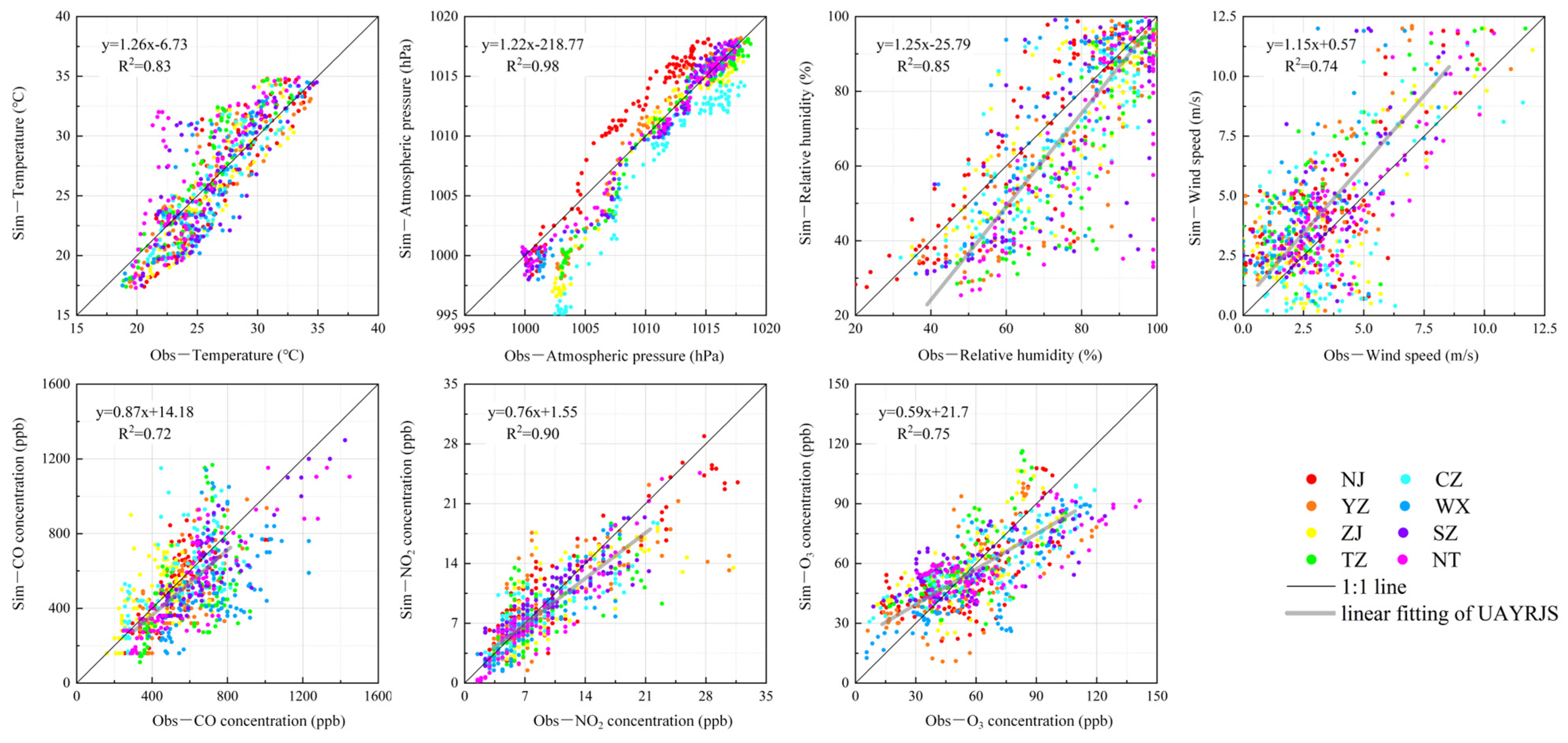
2.5. Evaluation of the Model Results

The simulated concentration by the WRF-CMAQ model was tested using the ozone concentration monitored by the national control points, and the evaluation indicators included the correlation coefficient (R) and root mean square error (RMSE) (see Equations (1) and (2)).
R = i = 1 N S i m i S i m ¯ O b s i O b s ¯ i = 1 N S i m i S i m ¯ 2 i = 1 N O b s i O b s ¯ 2
R M S E = i = 1 N S i m i O b s i 2 N
where N is the number of samples; S i m i   a n d   O b s i are the model simulation results and monitoring data results at i time, respectively; and S i m ¯   a n d   O b s ¯ are the averages of the simulation and monitoring results at i time.

3. Results and Discussion

3.1. Model Simulation Evaluation

As outlined in Section 2.1, this study utilized hourly data on air temperature, sea level pressure, relative humidity and instantaneous surface wind speed monitored by meteorological stations in the UAYRJS region between 00:00 on 4 September and 23:00 on 8 September 2022. The data were employed to assess the efficacy of the WRF simulation. Additionally, the hourly concentrations of CO, NO2 and O3 were obtained from air pollutant monitoring stations to evaluate the effectiveness of the WRF-CMAQ simulation. Figure 1 illustrates the locations of UAYRJS cities.
For the study period, statistical analysis was conducted for each variable, including mean deviation, mean absolute error (MAE), root mean square error (RMSE) and correlation coefficient (R). The averaged results for the UAYRJS region are presented in Figure 2 and Table 2. Overall, the simulated wind speeds were slightly higher than the observed values, with a mean deviation of 1.06 m/s. The simulated air temperatures and sea level pressures generally agreed with the monitored values, exhibiting a mean deviation of less than 0.5%. However, the other variables showed slightly lower values compared to the observations, with mean deviations ranging from 10% to 20%.
The R for all variables was greater than 0.6. In particular, the R values for sea level pressure, O3 concentration, relative humidity and air temperature were 0.99, 0.94, 0.92 and 0.91, respectively. These high R values indicate that the WRF and WRF-CMAQ models effectively reproduced the weather processes and characteristics of atmospheric pollutants. The biases of the simulated O3 concentrations in this study are comparable to or even smaller than previous studies [15,21,22,24,40].

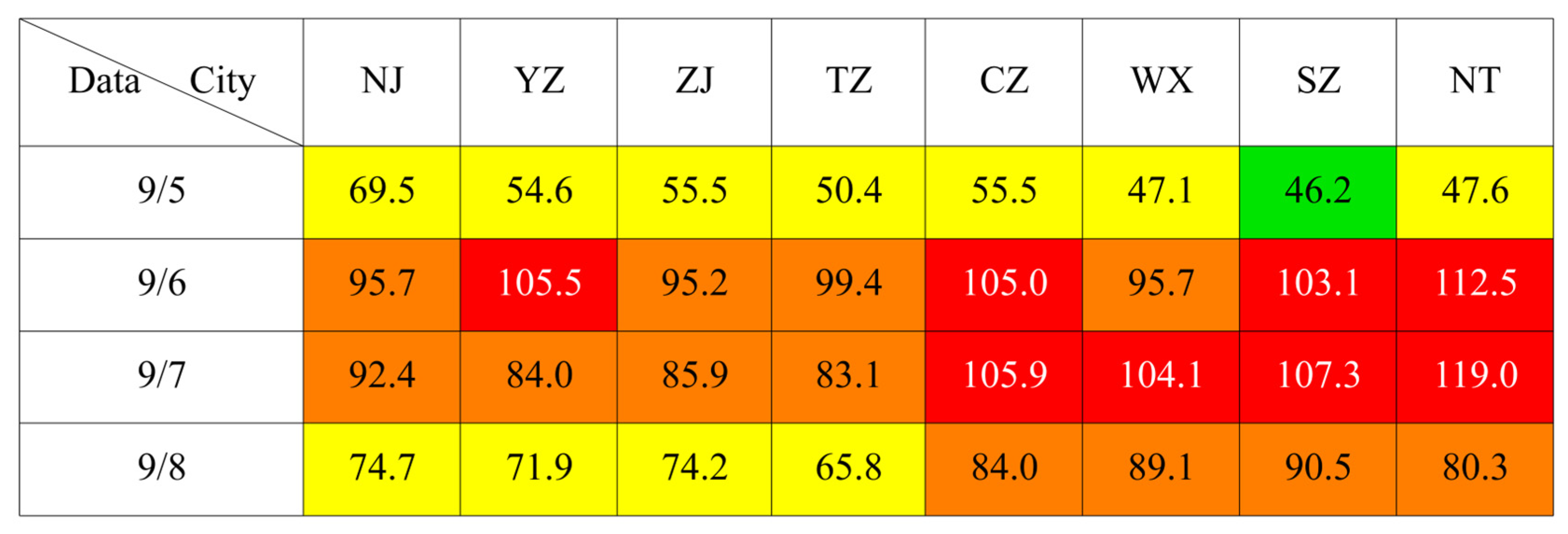
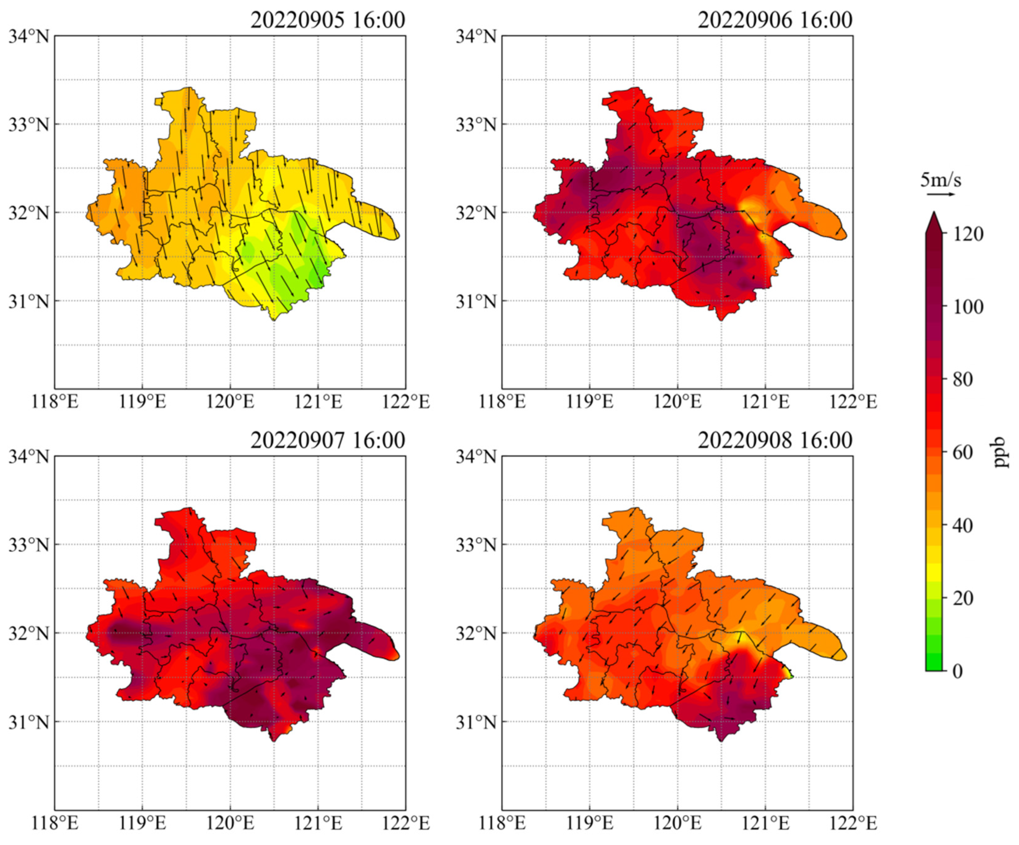
3.2. Analysis of the Variation Characteristics of Pollutants and the Weather Situation during the Contamination Process

The O3–8 h in UAYRJS from 5 to 8 September 2022 is shown in Figure 3, and ozone pollution was the most serious on 6–7 September, in which CZ, SZ and NT were moderately polluted on two consecutive days, and YZ and WX were moderately polluted on one day. On 8 September, O3–8 h was lower than that of the previous two days, but there were still five cities with light pollution.
Usually, the position of the 588 dgpm isopotential height line (referred to as the 588 line) is used to represent the intensity change of the western Pacific subtropical high (WPSH) [41]. In this study, the ozone polluted cities in the UAYRJS on different days, all located in the area encompassed by the contour 588 line, which was impacted by the WPSH, and it showed a good relationship between the control range of the WPSH and the ozone pollution area. We examined the changes in the 588 line at 16:00 every day from 5 to 8 September (Figure 4) and combined them with the ozone hourly concentration and surface wind field of the UAYRJS at 16:00 every day from 5 to 8 September, simulated by WRF-CMAQ (Figure 5). On 5 September, line 588 was located in the East China Sea. The ozone concentration was below 69.5 ppb and the dominant wind direction was north. On 6 September, the WPSH strengthened, and line 588 moved northward to 30° N. The ozone concentration generally exceeded 93.3 ppb and all of the UAYRJS cities exceeded the ozone standard (75.1 ppb); YZ, CZ, SZ and NT even showed moderate pollution that exceeded 103.1 ppb. The winds shifted to the south, and their speed was generally lower than 2 m s−1. At low wind speeds, air masses do not spread easily. It mainly affected the cities in the center of the region and the downwind cities, such as YZ, CZ, SZ and NT, so there was more serious ozone pollution in those cities. On 7 September, line 588 continued to move northward to 34° N and covered all of UAYRJS. In addition, all eight cities in the UAYRJS suffered light and moderate ozone pollution; and for CZ, WX, SZ, NT, all four cities exacerbated pollution by 0.9–8.4 ppb, with the highest reaching 107.3 ppb, showing a stable polluted state in the UAYRJS. The northern cities in UAYRJS, such as YZ, NJ and TZ, had a north wind, but in the southern cities, such as NT, SZ and WX, south winds prevailed, with wind speeds below 1 m s−1. South and north winds converged in CZ, WX, SZ and NT, so ozone concentrations were higher in these cities than in others. On 8 September, the WPSH weakened, and line 588 retreated to 30° N and the ozone concentration in UAYRJS dropped to 56 ppb; only SZ and the south of WX were still higher than 93.3 ppb, and the north wind gradually strengthened to about 4 m s−1. During the ozone event, in NJ and ZJ for example, located in the westernmost part of the UAYRJS, were less affected by the transmission of polluted air masses in the UAYRJS, and their ozone concentrations were lower than those of neighboring cities, such as CZ.

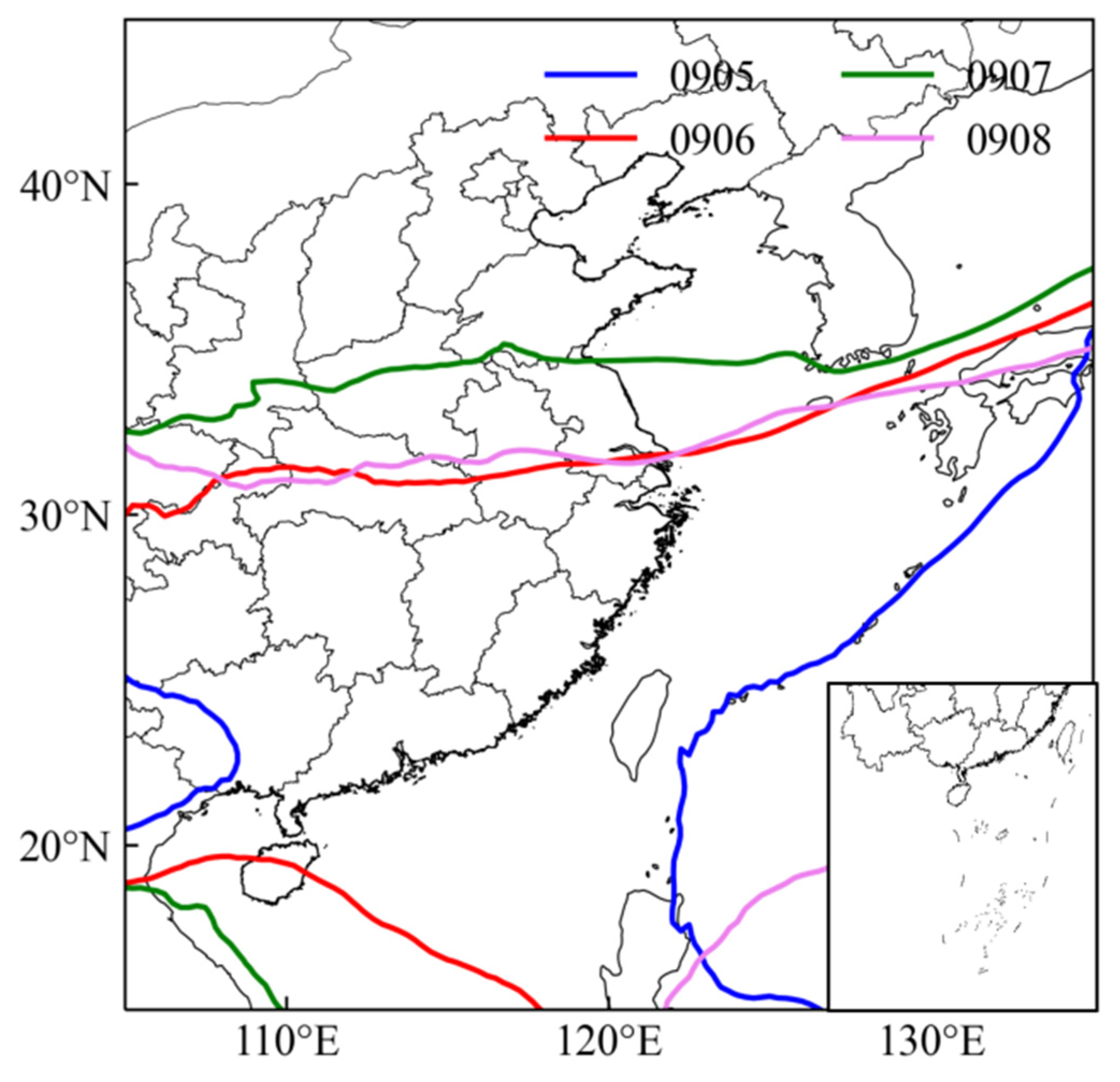
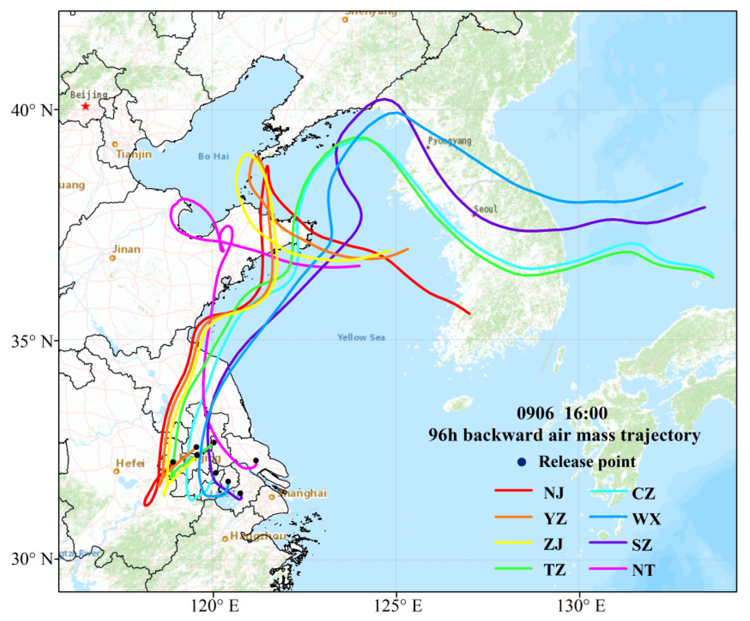
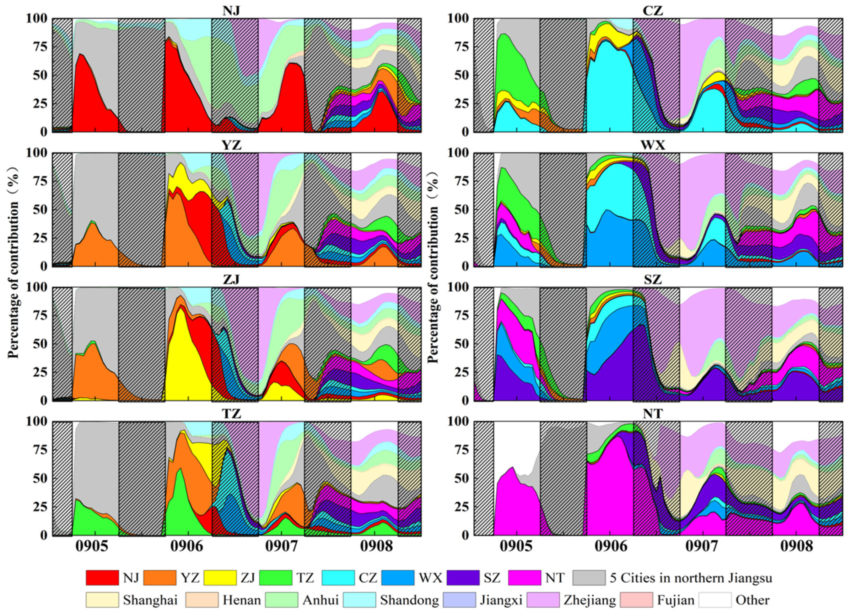
3.3. Transmission Path Analysis
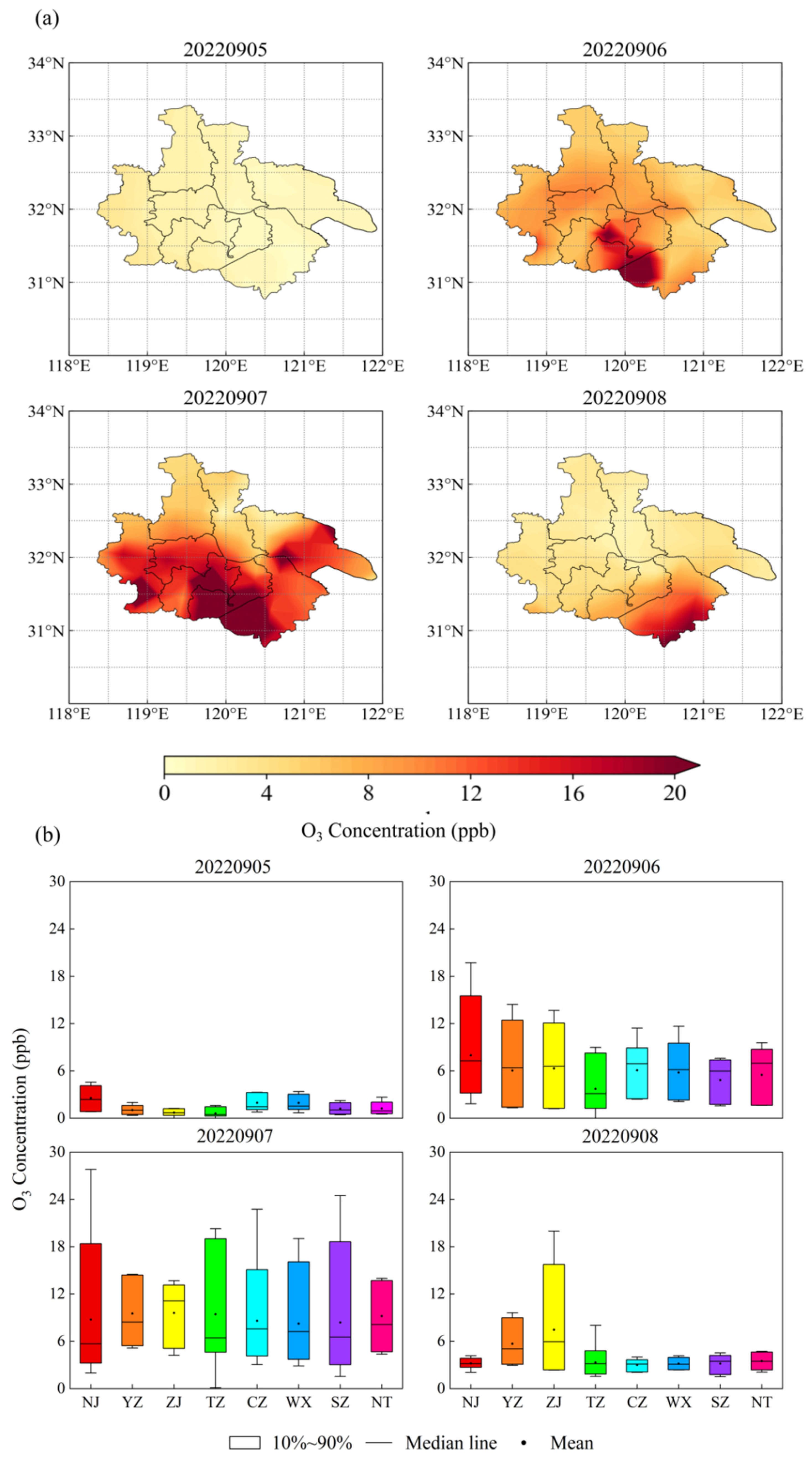
As shown in Section 3.2, it is clear that 6 September was the first polluted day of UAYRJS, and there was an enhanced WPSH process from 5 to 6 September. Furthermore, the main wind direction changed from north on 5 September to south on 6 September. The daily anthropogenic emission sources usually stayed in a steady state, but the weather conditions changed day by day, especially the air mass source. In order to analyze why the pollution event was triggered on 6 September, we used the HYSPLIT model to analyze the air mass transport paths of pollution in the UAYRJS at 16:00 on the day (Figure 6). The air masses arriving at the research area at the time were all from the Yellow Sea and the Bohai Sea first of all; second, they passed through Shandong Province and to the north of Jiangsu Province, and got to UAYRJS; finally, they returned to UAYRJS after passing through Anhui Province in a southerly direction.
According to the air mass path estimate, pollution may have a transmission impact in the ocean, Shandong, northern Jiangsu and Anhui.

3.4. Ozone Sources

To further quantify the impact of anthropogenic emissions and regional pollution transport, we evaluated the hourly contributions of neighboring provinces (Shanghai, Henan, Anhui, Shandong, Jiangxi, Zhejiang and Fujian), five cities in northern Jiangsu and other regions (including the ocean) to ozone concentrations in the UAYRJS from 5 to 8 September using the CMAQ-ISAM module (Figure 7). From the observed data, the ozone hourly concentrations in UAYRJS ranged from 36.4 to 92.6 ppb during the daytime (7:00–17:00) and from 37.7 to 74 ppb during the nighttime (18:00–6:00 the next day), and the average nighttime concentration was lower than that of the daytime average concentration by 13.3 ppb.
From the daytime hourly contribution results, NJ, YZ, ZJ, TZ and NT were mainly affected by local generation on 5 September, with a contribution share of 30–70% and a contribution concentration range of 9.3–30.3 ppb, followed mainly by the contribution from the five cities in northern Jiangsu Province and other regions. Suzhou, WZ and CZ were affected by intra-regional transmission from UAYRJS, contributing 25–65% and 4.7–23.3 ppb; for example, CZ generated 25%, and TZ, ZJ and other cities contributed up to 50%.
On 6 September, ozone in the UAYRJS was dominated by intra-city generation and intra-regional transmission, which together accounted for 75–98% of the total. Among them, ozone in NJ was mainly generated in the city, with the highest city hourly contribution of up to 80%, contributing to the concentration of 37.3 ppb, while the extra-regional contribution was mainly from Anhui, Shandong and five cities in northern Jiangsu. As for the other seven cities, the contribution of local ozone generation accounted for 25–75%, and the concentration contribution was in the range of 9.3–98 ppb; compared with 5 September, the contribution of intra-regional transmission to local ozone increased to differing degrees, and the concentration contribution increased by about 2.3–28 ppb (5–20%). Among them, the intra-regional transmissions from SZ, WX, CZ and TZ were prominent, with a contribution of up to 60%.
On 7 September, the ozone pollution in UAYRJS was dominated by an extra-regional contribution, up to 70%, and a contributing concentration in the range of 4.7–70 ppb. Among them, NJ, YZ, ZJ and TZ were mainly affected by the contribution of Anhui Province, and secondly, by the influences of Zhejiang Province and the five northern cities of Jiangsu Province; CZ, WX, SZ and NT were mainly affected by Zhejiang Province, followed by Shanghai, Shandong and other regions (ocean, etc.).
On 8 September, compared with the previous day, single city contributions were down to about 20%, intra-regional transmission contributions were in the range of 30–55%, contributing to a concentration of 2.3–23.3 ppb, and the contribution of extra-regional transmission was mainly from the five cities of northern Jiangsu Province, Shanghai and Zhejiang Province (accounting for about 50%), contributing to a concentration of 4.7–16.3 ppb.
In the nighttime, the ozone source in the UAYRJS was different from the daytime. On 5 September, ozone in UAYRJS was mainly affected by extra-regional transmission, dominated by transmission from the five cities in northern Jiangsu Province, with a contribution range of 65% to 90% and a contribution concentration of 9.3–60.7 ppb.
On 6 September, ozone in UAYRJS was dominated by both the city and intra-regional contributions, with a combined share ranging from 50 to 95% and a contribution concentration of 18.7–88.7 ppb. Extra-regional transmission was dominated by Zhejiang Province, with a contribution share of 20–70% and a contribution concentration of 2.3–32.7 ppb.
On 7 and 8 September, ozone in UAYRJS was dominated by extra-regional transmission, with a contribution share of 50–80% and a contribution concentration of 14–65.3 ppb, which was dominated by the five cities in Jiangsu Province, Shanghai and Zhejiang Province and an intra-region contribution share of 10–25%, with a contribution concentration of 0.9–3.7 ppb. The contribution from cities in UAYRJS was less than 15%, with a contribution to the concentration of 0.5–3.7 ppb.
Overall, there was no ozone pollution on 5 September, and the UAYRJS cities were the main contributors during the day (accounting for 30–70%), while at night, extra-regional sources, such as the five cities in northern Jiangsu Province, were the main contributors, accounting for 65–90%. This was followed by a marked pollution transmission phenomenon on 6 and 7 September, with predominantly intra-regional contributions from the UAYRJS cities on 6 September, accounting for 50–98%, and extra-regional transmission dominating on 7 September, with a contribution of 50–80%. It indicated that the high ozone values were primarily due to transport; secondary causes have been due to a local accumulation of ozone due to photochemical reactions. Finally, on 8 September, the city and intra-regional contributions were further reduced, and the extra-regional contribution of the five cities in northern Jiangsu Province, Shanghai and other areas dominated, with a contribution of about 67%.

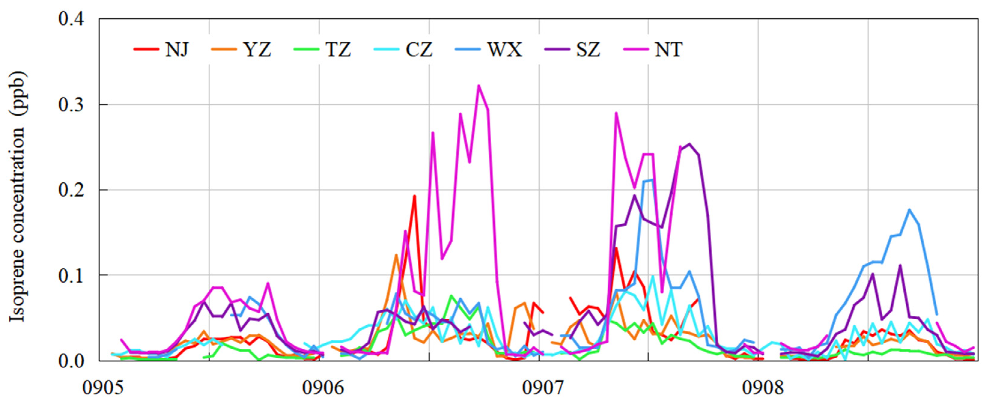
3.5. BVOCs Contributions

Volatile organic compounds are important precursors for the formation of ozone, and their sources can be divided into AVOCs and BVOCs. Biogenic VOCs are 2–3 times more chemically reactive than AVOCs and, once emitted, rapidly react with atmospheric oxidants (e.g., OH) to produce oxidizing products such as ozone, which can significantly affect air quality even at low volume fraction levels [42]. The Jiangsu, Zhejiang and Fujian regions have high vegetation cover and, therefore, higher BVOCs emissions. In addition, this region has high NOx volume fractions, and some studies have suggested that the potential impact of BVOCs on ozone may be further amplified [43].
Isoprene is the most abundant non-methane VOC worldwide and one of the precursors of ozone generation [44,45,46]. It has high atmospheric activity, with a lifetime in the atmosphere of only 1–2 h [47]. Thus, it is an essential photochemical reagent. In this study, isoprene was used to represent BVOCs. This study addresses the role of BVOCs in this pollution process by analyzing the changes in hourly observed isoprene concentrations in the UAYRJS from 5 to 8 September (Figure 8). Because the eight sites were generally located in areas with urban, hardened surfaces and less vegetation covered around the sites, the observed isoprene concentrations were lower than 0.4 ppbv. In the countryside, the isoprene concentrations could be higher than 1 ppbv [15]. It was higher than the concentration in the city center. On 5 September, the hourly peak isoprene concentrations in SZ, WX and NT were around 0.09 ppb, and the other cities were below 0.06 ppb. On 6 September, the peak hourly isoprene concentration in NT was the highest, reaching 0.32 ppb, followed by NJ (0.19 ppb); the other six cities all had different degrees of increase compared to the previous day. On 7 September, the hourly peak concentrations in NT and SZ were the highest, at 0.29 ppb and 0.26 ppb, respectively, and the peaks in the other cities were close to those of the previous day. On 8 September, the hourly peak concentrations in all eight cities decreased, with a maximum below 0.18 ppb. The isoprene concentrations in UAYRJS on 6 and 7 September were higher than those on the other two days by about 0.10–0.20 ppb, and the contribution of the emissions of BVOCs to the ozone pollution of UAYRJS during this period was relatively clear.
To further quantify the impact of BVOCs emissions on ozone concentrations in the study area, we utilized the WRF-CMAQ model in conjunction with the biogenic emissions model MEGAN to conduct two sets of control experiments: Scenario 1 (S1) was the basic scenario, which considered both anthropogenic and biogenic emissions to simulate the emissions of BVOCs during the pollution process; Scenario 2 (S2) was a sensitivity test that considered only anthropogenic emissions and ignored biogenic emissions. These two scenarios kept the same parameter settings, except for the difference between biogenic emissions, and the difference between the simulation results could be used to quantitatively assess the contribution of BVOCs to ozone pollution. The parameter settings of this simulation experiment were consistent with prior research by Wang et al. [20].
Figure 9a,b shows the spatial distribution of the simulated daily contribution values of biogenic emissions to ozone and the hourly ozone concentration contribution (the difference between the simulation results of S1 and the ozone concentrations derived from S2) from 5 to 8 September, 2022, in the UAYRJS, respectively. From the spatial distribution, on 5 September, the contribution value of biogenic emissions to ozone was relatively small in UAYRJS, below 4.7 ppb. On 6 September, the highest contribution was concentrated in the southern UAYRJS, exceeding 11.7 ppb, and the contribution of biogenic sources in localized areas of ZJ, CZ and WX increased rapidly to about 11.7–25.7 ppb, while the other five cities contributed to concentrations of between 9.3 and 16.3 ppb. On 7 September, the range of high-value areas was further expanded, with high value contribution areas occurring in NJ, SZ, WX, CZ and NT, with concentrations above 23.3 ppb; ZJ contributed concentrations between 11.7 and 21 ppb, and YZ and TZ BVOCs contributed concentrations not exceeding 11.7 ppb. On 8 September, the high contribution value areas showed a tendency to move to the southeast, with only the southern part of SZ reaching 23.3 ppb, the contribution in other areas was lower than 9.3 ppb.
From the hourly BVOCs contribution to ozone concentrations in the UAYRJS, BVOCs contributed positively to ozone concentrations in all eight cities from 5 to 8 September. On 5 September, the contribution concentrations of the UAYRJS were below 4.7 ppb, and the daily average ozone concentration contributed by BVOCs accounted for 1.5–8.3%. The average hourly contribution was 0.2–19.7 ppb and 0.1–27.8 ppb, respectively, and the contribution to ozone concentration on that day was 7.6–19.1%. Except for ZJ, the contribution of BVOCs decreased to below 9.3 ppb on 8 September, accounting for about 6% of the city’s ozone concentration. The higher BVOCs emissions on 6 and 7 September were an important cause of the serious ozone pollution in the UAYRJS. However, owing to the significant impact of emission factors on improving emission estimation and air quality prediction in areas with rich vegetation, there is uncertainty in the default emission factor [38], and this result needs to be further considered.

4. Conclusions

The causes of ozone pollution in UAYRJS from 6 to 8 September 2022 were analyzed from the perspectives of the weather situation, regional transmission contribution and BVOCs emission contribution. The main conclusions are as follows:
During the ozone pollution event, the weather situation in the region was controlled by the WPSH, which had an adverse effect on pollution. The backward trajectory of the air mass indicated that all cities in the study area were affected by polluted air masses transmitted from the UAYRJS, the regional provinces and the ocean. The results of WRF-CMAQ-ISAM showed that, on 6 September, the cities in the UAYRJS and the transmission within the region were the main contributors to the ozone pollution (50–98%), while on 7 September, the contribution of extra-regional transmission was the main contributor, accounting for 50–80%, with the polluted air mass outside the region aggravating the ozone pollution in the UAYRJS.
The observed isoprene concentrations in each city on 6 and 7 September were 0.03–0.1 ppb higher than those on 5 and 8 September, and the concentrations in NT, WX, SZ, CZ and NJ increased significantly. The results of the sensitivity test showed that, first, the contribution of BVOC emissions to ozone pollution in the UAYRJS was 7.6%–19.1% on 6 and 7 September. Second, the spatial variation of the area with the high concentration of BVOCs contribution (difference of ozone concentration > 23.3 ppb) from 6 to 8 September was consistent with that of the ozone pollution area, which was concentrated in SZ, WX and CZ on 6 September and then expanded to include almost all cities in the region on 7 September and moved to the south of the region on 8 September.
This heavy ozone pollution event was one of the most severe pollutions in the UAYRJS during the same period in history. This study utilized this prominent case of ozone pollution as an entry point to investigate the accumulation of ozone concentrations in UAYRJS, with a particular focus on the influence of the weather situation, inland and coastal transport, the contribution of upstream cities and the BVOCs contribution. The study demonstrated that interregional ozone transport in UAYRJS had a greater than 50% impact on influencing ozone concentration exceedances. Furthermore, in addition to the contribution of AVOCs to ozone, the BVOCs contribution should not be underestimated (up to 25.7 ppb for the highest hourly concentration). The findings of this study provide a scientific basis for future research on the impact of substance emissions on ozone pollution and interregional joint prevention and control of ozone pollution. The causes of ozone pollution in the UAYRJS are relatively complex and require further in-depth study.

Author Contributions

Conceptualization, Z.C., D.Z., J.Y., S.Z. and L.Z.; methodology, Z.C., D.Z. and F.J.; software, L.Z. and Z.T.; validation, Z.C., D.Z. and Z.L.; formal analysis, D.Z. and L.Z.; investigation D.Z., F.J. and Z.C.; resources, J.Y., S.Z. and L.Z.; data curation, J.Y. and S.Z.; writing—original draft preparation, Z.C.; D.Z., J.Y., S.Z. and Z.L; writing—review and editing, D.Z., F.J. and Z.C.; visualization, Z.L. and Z.T.; supervision, Z.C. and D.Z.; project administration, D.Z. and F.J.; funding acquisition, D.Z. and F.J. All authors have read and agreed to the published version of the manuscript.

Funding

This research was funded by National Key Research and Development Program of China, grant number 2023YFC3709401, Jiangsu Provincial Science Fund for Distinguished Young Scholars, grant number BK20231530 and the Joint Fund of the Zhejiang Provincial Natural Science Foundation of China, grant number LZJMZ24D050008.

Data Availability Statement

The ozone observation data can be found here https://air.cnemc.cn:18007/ (accessed on 26 September 2022). The meteorological data can be found here https://cds.climate.copernicus.eu/ (accessed on 28 September 2022) and http://rda.ucar.edu/datasets/ds083.2/ (accessed 28 September 2022). The other data presented in this study, such as the isoprene concentrations are available on request from the corresponding author.

Acknowledgments

All authors have read and agreed to the published version of the manuscript. We acknowledge all the anonymous reviewers for their comments to improve the original manuscript.

Conflicts of Interest

Authors Zhe Cai, Longfei Zheng, Zijun Luo and Zhiwei Tang were employed by the company Nanjing Climblue Technology Co. The remaining authors declare that the research was conducted in the absence of any commercial or financial relationships that could be construed as a potential conflict of interest.

References

  1. Guo, Y.H. Spatiotemporal Pattern and Health Impact Assessment of Ozone Pollution in China; North-West University: Potchefstroom, South Africa, 2022. [Google Scholar]
  2. Zhao, Y.; Li, Y.; Kumar, A.; Ying, Q.; Vandenberghe, F.; Kleeman, M.J. Separately resolving NOx and VOC contributions to ozone formation. Atmos. Environ. 2022, 285, 119224. [Google Scholar] [CrossRef]
  3. Wan, W.X.; Zhang, S.H.; Li, J.; Sun, X.; Guan, Z.G.; Yu, X.H.; Yang, Y.H.; Wang, X.K. Regional differences in urban air ozone pollution and its damage to plants in Hebei Province. J. Ecol. Environ. Sci. 2021, 30, 2185–2194. [Google Scholar]
  4. Peng, L.; Li, Q.; Cai, Q.W.; Qiu, X.H. Impact of ozone on the yield and economic benefits of major food crops in China from 2015 to 2020. J. Saf. Environ. 2023, 23, 2958–2968. [Google Scholar]
  5. Wang, Y.; Song, Q.; Frei, M.; Shao, Z.; Yang, L. Effects of elevated ozone, carbon dioxide, and the combination of both on the grain quality of Chinese hybrid rice. Environ. Pol. 2014, 189, 9–17. [Google Scholar] [CrossRef] [PubMed]
  6. Monks, P.S.; Archibald, A.T.; Colette, A.; Cooper, O.; Coyle, M.; Derwent, R.; Fowler, D.; Granier, C.; Law, K.S.; Mills, G.E.; et al. Tropospheric ozone and its precursors from the urban to the global scale from air quality to short-lived climate forcer. Atmos. Chem. Phys. 2015, 15, 8889–8973. [Google Scholar] [CrossRef]
  7. Wu, Y.; Gu, J.; Shi, X.; Shen, W.; Zhang, H.; Zhang, X. Characteristics and formation mechanism of ozone pollution in demonstration zone of the Yangtze River Delta, China. Atmosphere 2024, 15, 382. [Google Scholar] [CrossRef]
  8. Shen, Y.; Liu, J.; Chen, Z.; Yang, M.; Shu, L.; Gai, C.; Jiang, Y. Influence of wind flows on surface O3 variation over a coastal province in Southeast China. Atmosphere 2024, 15, 262. [Google Scholar] [CrossRef]
  9. Zheng, S.C.; Jiang, F.; Feng, S.Z.; Liu, H.; Wang, X.Y.; Tian, X.D.; Ying, C.Y.; Jia, M.W.; Shen, Y.; Lyu, X.P.; et al. Impact of Marine Shipping Emissions on Ozone Pollution during the Warm Seasons in China. J. Geophys. Res. Atmos. 2024, 129, e2024JD040864. [Google Scholar] [CrossRef]
  10. Lyu, X.; Wang, N.; Guo, H.; Xue, L.; Jiang, F.; Zeren, Y.; Cheng, H.; Cai, Z.; Han, L.; Zhou, Y. Causes of a continuous summertime O3 pollution event in Jinan, a central city in the North China Plain. Atmos. Chem. Phys. 2019, 19, 3025–3042. [Google Scholar] [CrossRef]
  11. Hua, X.; Wang, M.; Yao, Z.; Hao, R.; Wang, H. Characteristics and sensitivity analysis of ozone pollution in a typical inland city in China. Atmosphere 2024, 15, 160. [Google Scholar] [CrossRef]
  12. Zhang, Y.; Gao, J.; Zhu, Y.; Liu, Y.; Li, H.; Yang, X.; Zhong, X.; Zhao, M.; Wang, W.; Che, F.; et al. Evolution of ozone formation sensitivity during a persistent regional ozone episode in Northeastern China and its implication for a control strategy. Environ. Sci. Technol. 2024, 58, 617–627. [Google Scholar] [CrossRef] [PubMed]
  13. Min, Z. Study on the Characteristics and Generation Mechanism of Ozone Pollution in Typical Delta Cities; Shandong University: Jinan, China, 2022. [Google Scholar]
  14. Lu, D.; Li, H.; Tian, M.; Wang, G.; Qin, X.; Zhao, N.; Huo, J.; Yang, F.; Lin, Y.; Chen, J.; et al. Secondary aerosol formation during a special dust transport event: Impacts from unusually enhanced ozone and dust backflows over the ocean. Atmos. Chem. Phys. 2023, 23, 13853–13868. [Google Scholar] [CrossRef]
  15. Lou, C.X.; Jiang, F.; Tian, Q.L.; Zheng, Y.H.; Zou, X.; Shen, Y.; Feng, S.Z.; Chen, J.S.; Zhang, L.Y.; Jia, M.W.; et al. Modeling the biogenic isoprene emissions and its impact on ozone pollution over Zhejiang province, China. Sci. Total Environ. 2022, 865, 161212. [Google Scholar] [CrossRef] [PubMed]
  16. Lu, X.; Zhang, L.; Chen, Y.; Zhou, M.; Zheng, B.; Li, K.; Liu, Y.; Lin, J.; Fu, T.-M.; Zhang, Q. Exploring 2016–2017 surface ozone pollution over China: Source contributions and meteorological influences. Atmos. Chem. Phys. 2019, 19, 8339–8361. [Google Scholar] [CrossRef]
  17. Ge, Q.; Zhang, X.S.; Cai, K.; Liu, Y. Ozone pollution in Chinese cities: Spatiotemporal variations and their relationships with meteorological and other pollution factors (2016–2020). Atmosphere 2022, 13, 908. [Google Scholar] [CrossRef]
  18. Zhang, X.; Zhou, L.; Zhang, X.; Luo, Y.; Sun, L. A case study on the impact of East Asian summer monsoon on surface O3 in China. Atmosphere 2023, 14, 768. [Google Scholar] [CrossRef]
  19. Shu, L.; Xie, M.; Wang, T.J.; Gao, D.; Chen, P.L.; Han, Y.; Li, S.; Zhuang, B.L.; Meng, M. Integrated studies of a regional ozone pollution synthetically affected by subtropical high and typhoon system in the Yangtze River Delta region, China. Atmos. Chem. Phys. 2016, 16, 15801–15819. [Google Scholar] [CrossRef]
  20. Yi, R.; Wang, Y.L.; Zhang, Y.J.; Zhang, Y.J.; Shi, Y.; Li, M.S. Analysis of urban ozone pollution characteristics and influencing factors in the Yangtze River Delta. J. Environ. Sci. 2015, 35, 2370–2377. [Google Scholar]
  21. Zheng, Y.; Jiang, F.; Feng, S.; Shen, Y.; Liu, H.; Guo, H.; Lyu, X.; Jia, M.; Lou, C. Large-scale land-sea interactions extend ozone pollution duration in coastal cities along northern China. Environ. Sci. Ecotechnol. 2024, 18, 100322. [Google Scholar] [CrossRef]
  22. Ying, C.Y.; Lin, J.; Zheng, W.F.; Cai, Z.; Chen, X.; Tang, Z.W.; Zhou, D.R.; Jiang, F. Causes and control measures of ozone pollution in Fuzhou city under the influence of typhoon ‘Nanmadu’. Res. Environ. Sci. 2023, 36, 2293–2305. [Google Scholar] [CrossRef]
  23. Shen, Y.; Jiang, F.; Feng, S.Z.; Xia, Z.; Zheng, Y.H.; Lyu, X.; Zhang, L.Y.; Lou, C.X. Increased diurnal difference of NO2 concentrations and its impact on recent ozone pollution in eastern China in summer. Sci. Total Environ. 2023, 858, 159767. [Google Scholar] [CrossRef] [PubMed]
  24. Zhou, D.R.; Liu, Y.; Gao, J.; Tang, Z.W.; Cai, Z.; Huang, X.; Qin, L. Sensitivity to prevention and control and emission reduction scenarios of typical ozone pollution processes in eastern China. J. Atmos. Sci. 2023, 46, 667–678. [Google Scholar]
  25. Lyu, X.P.; Li, K.; Guo, H.; Morawska, L.; Zhou, B.; Zeren, Y.; Jiang, F.; Chen, C.; Goldstein, A.H.; Xu, X.; et al. A synergistic ozone-climate control to address emerging ozone pollution challenges. One Earth 2023, 6, 964–977. [Google Scholar] [CrossRef]
  26. Zhou, D.R.; Tian, X.D.; Cai, Z.; Wang, X.Y.; Li, Y.; Liu, Y.; Jiang, F. Evaluation of ozone change and control effect in Yangtze River Delta region during the G20 summit. China Environ. Moni 2020, 36, 41–49. [Google Scholar]
  27. Chu, C.J.; Liang, J.; Yu, J.H.; Cai, Z.; Liu, Y. Characteristics and causes of primary ozone heavy pollution in the Yangtze River area of Jiangsu Province. Sichuan Environ. 2022, 76–83. [Google Scholar] [CrossRef]
  28. Yu, J.H.; Cai, Z.; Liu, Y.; Chen, A.Q. Case study of heavy ozone pollution in Jiangsu Province based on WRF-CMAQ-ISAM: A case study of a severe pollution in Huai’an City at the end of May 2021. Sichuan Environ. 2022, 41, 74–80. [Google Scholar]
  29. Sun, D.; Si, Y.D.; Wang, H.; Wu, J.X. Analysis of typical ozone pollution process in inland cities in northern Jiangsu in the summer of 2019. Environ. Prot. Cir. Econ. 2022, 42, 76–79, 82. [Google Scholar]
  30. GB3095–2012; Ambient Air Quality Standards. The Ministry of Environmental Protection (MEP): Beijing, China, 2012.
  31. MEP. Technical Regulation for Selection of Ambient Air Quality Monitoring Stations (on Trial); The Ministry of Environmental Protection (MEP): Beijing, China, 2013. [Google Scholar]
  32. Muñoz-Sabater, J.; Dutra, E.; Agustí-Panareda, A.; Albergel, C.; Arduini, G.; Balsamo, G.; Boussetta, S.; Choulga, M.; Harrigan, S.; Hersbach, H.; et al. ERA5-Land: A state-of-the-art global reanalysis dataset for land applications. Ear Syst. Sci. Dat. 2021, 13, 4349–4383. [Google Scholar] [CrossRef]
  33. Skamarock, W.C.; Klemp, J.B.; Dudhia, J.; Gill, D.O.; Liu, Z.; Berner, J.; Wang, W.; Powers, J.G.; Duda, M.G.; Barker, D.; et al. A Description of the Advanced Research WRF Model Version 4No; National Center for Atmospheric Research/TN-556+STR; National Center for Atmospheric Research: Boulder, America, 2019. [Google Scholar] [CrossRef]
  34. Yang, J.; Duan, K. Effects of initial drivers and land use on Wrf modeling for near-surface fields and atmospheric boundary layer over the Northeastern Tibetan Plateau. Adv. Meteorol. 2016, 2016, 7849249. [Google Scholar] [CrossRef]
  35. Wang, N.; Guo, H.; Jiang, F.; Ling, Z.H.; Wang, T. Simulation of ozone formation at different elevations in mountainous area of Hong Kong using WRF-CMAQ model. Sci. Total Environ. 2015, 505, 939–951. [Google Scholar] [CrossRef]
  36. Kwok, R.H.F.; Napelenok, S.L.; Baker, K.R. Implementation and evaluation of PM2.5 source contribution analysis in a photochemical model. Atmos. Environ. 2013, 80, 398–407. [Google Scholar] [CrossRef]
  37. Kwok, R.H.F.; Baker, K.R.; Napelenok, S.L.; Tonnesen, G.S. Photochemical grid model implementation and application of VOC, NOx, and O3 source apportionment. Geosci. Model Dev. 2015, 8, 99–114. [Google Scholar] [CrossRef]
  38. Peng, W.; Zhang, Y.L.; Gong, H.X.; Zhang, H.L.; Guenther, A.; Zeng, J.Q.; Wang, T.; Wang, X.M. Updating biogenic volatile organic compound (BVOC) emissions with locally measured emission factors in South China and the effect on modeled ozone and secondary organic aerosol production. J. Geophys. Res. Atmos. 2023, 128, e2023JD039928. [Google Scholar] [CrossRef]
  39. Stein, A.F.; Draxler, R.R.; Rolph, G.D.; Stunder, B.J.; Cohen, M.D.; Ngan, F. NOAA’s HYSPLIT atmospheric transport and dispersion modeling system. Bull. Am. Meteorol. Soc. 2016, 96, 2059–2077. [Google Scholar] [CrossRef]
  40. Zheng, Y.; Jiang, F.; Feng, S.; Cai, Z.; Shen, Y.; Ying, C.; Wang, X.; Liu, Q. Long–Range Transport of Ozone across the Eastern China Seas: A Case Study in Coastal Cities in southeastern China. Sci. Total Environ. 2021, 768, 144520. [Google Scholar] [CrossRef] [PubMed]
  41. Na, Y.; Wang, J.; Zhang, Y.J.; Zhang, P.Q.; Lu, R.Y. Establishment and application of segmented subtropical high position index. Metro 2022, 48, 1439–1448. [Google Scholar]
  42. Zhang, M.M.; Shao, M.; Chen, P.L.; Gu, C.; Wang, Q.Y. Comparative study on the emission characteristics of VOCs from anthropogenic and natural sources in the Yangtze River Delta region and their impact potential on atmospheric O3 and SOA[J/OL]. China Environ. Sci. 2023, 43, 2694–2702. [Google Scholar] [CrossRef]
  43. Wu, K.; Yang, X.; Chen, D.; Gu, S.; Lu, Y.; Jiang, Q.; Wang, K.; Ou, Y.; Qian, Y.; Shao, P.; et al. Estimation of biogenic VOC emissions and their corresponding impact on ozone and secondary organic aerosol formation in China. Atmos. Res. 2020, 231, 231104656. [Google Scholar] [CrossRef]
  44. Wang, N.; Huang, X.; Xu, J.; Wang, T.; Tan, Z.M.; Ding, A. Typhoon-boosted biogenic emission aggravates cross-regional ozone pollution in China. Sci. Adv. 2022, 8, 2. [Google Scholar] [CrossRef]
  45. Liu, Y.; Li, L.; An, J.; Huang, L.; Yan, R.; Huang, C.; Wang, H.; Wang, Q.; Wang, M.; Zhang, W. Estimation of biogenic VOC emissions and its impact on ozone formation over the Yangtze River Delta region, China. Atmos. Environ. 2018, 186, 113–128. [Google Scholar] [CrossRef]
  46. Jiang, F.; Zhou, P.; Liu, Q.; Wang, T.J.; Zhuang, B.L.; Wang, X.Y. Modeling tropospheric ozone formation over East China in springtime. J. Atmos. Chem. 2012, 69, 303–319. [Google Scholar] [CrossRef]
  47. Wennberg, P.O.; Bates, K.H.; Crounse, J.D.; Dodson, L.G.; McVay, R.C.; Mertens, L.A.; Nguyen, T.B.; Praske, E.; Schwantes, R.H.; Smarte, M.D.; et al. Gas-phase reactions of isoprene and its major oxidation products. Chem. Rev. 2018, 118, 3337–3390. [Google Scholar] [CrossRef] [PubMed]
Figure 1. Domain 02’s setting of WRF-CMAQ-ISAM model.
Atmosphere 15 00942 g001
Figure 2. Evaluation of the simulations of each variable hourly value in UAYRJS from 5 to 8 September 2022.
Atmosphere 15 00942 g002
Figure 3. O3–8 h pollution calendar map in UAYRJS from 5 to 8 September 2022 (unit: ppb). (Note: Green, yellow, orange and red represent excellent, good, light and moderate pollution under the ozone air quality sub-index standards, respectively).
Atmosphere 15 00942 g003
Figure 4. Height distribution of 588 dgpm potential at an altitude of 500 hPa on 16:00, 5 to 8 September 2022.
Atmosphere 15 00942 g004
Figure 5. Spatial distribution of ozone concentration changes in UAYRJS from 5 to 8 September 2022. (Note: The shades represent the concentration distribution, and the vector arrows represent the wind direction and speed).
Atmosphere 15 00942 g005
Figure 6. 96 h backward trajectories of UAYRJS at 16:00 on 6 September 2022. (Note: The dots represent the simulated release position; the lines represent the spatial distribution of traceable trajectories).
Atmosphere 15 00942 g006
Figure 7. Hourly series of ozone source analysis in UAYRJS from 5 to 8 September 2022. (Note: The superimposed slash mask area represents the nighttime, with no mask for daytime. The coloring map depicts the relative contribution from different regions represented by different colors to the hourly concentration in a given city; they add up to a total of 100%. The highly saturated colors represent the UAYRJS, and relatively low saturation represents other areas).
Atmosphere 15 00942 g007
Figure 8. Hourly observed concentration of isoprene in UAYRJS. (Data for ZJ are missing, so only seven cities’ concentration series are displayed).
Atmosphere 15 00942 g008
Figure 9. Spatial distribution of daily contribution concentrations (a) and hourly contribution concentration by city (b) to ozone from simulated sources in UAYRJS from 5 to 8 September 2022.
Atmosphere 15 00942 g009
Table 1. Configurations for physical and chemical parameterization in WRF-CMAQ.
Scheme NameScheme Settings
MicrophysicsPurdue Lin scheme
Cumulus convectionKain–Fritsch (new Eta) scheme
Longwave radiationRRTM scheme
Shortwave radiationGoddard shortwave
Sticky layerMonin-obukhov
Surface layerNoah Land Surface Model
Boundary layerYongsei University (YSU) scheme
Table 2. Evaluation of the simulations of each variable hourly value in UAYRJS from 5 to 8 September 2022. (Abbreviations were as follows: MAE, mean absolute error; R, coefficient of determination; RMSE, root mean square error).
VariablesMeanMAERRMSE
ObservationSimulation
Temperature (°C)26.0 25.9 −0.09 0.91 2.09
Sea level pressure (hPa)1011.0 1010.2 −0.81 0.99 1.63
Relative humidity (%)74.4 67.2 −7.23 0.92 11.53
Wind speed (m/s)3.3 4.3 1.06 0.86 1.73
CO (ppb)571.4 512.5 −58.92 0.85 102.44
NO2(ppb)9.2 7.5 −1.71 0.64 4.11
O3(ppb)125.9 106.6 −19.32 0.94 26.41
Disclaimer/Publisher’s Note: The statements, opinions and data contained in all publications are solely those of the individual author(s) and contributor(s) and not of MDPI and/or the editor(s). MDPI and/or the editor(s) disclaim responsibility for any injury to people or property resulting from any ideas, methods, instructions or products referred to in the content.

