Long-Term Variability of Surface Ozone and Its Associations with NO_x and Air Temperature Changes from Air Quality Monitoring at Belsk, Poland, 1995–2023

Abstract

Surface ozone (O₃) and nitrogen oxides (NO_x = NO + NO₂) measured at the rural station in Belsk (51.83° N, 20.79° E), Poland, over the period of 1995–2023, were examined for long-term variability of O₃ and its relationship to changes in the air temperature and NO_x. Negative and positive trends were found for the 95th and 5th percentile, respectively, in the O₃ data. A weak positive correlation (statistically significant) of 0.33 was calculated between O₃ and the temperature averaged from sunrise to sunset during the photoactive part of the year (April–September). Recently, O₃ maxima have become less sensitive to temperature changes, reducing the incidence of photochemical smog. The ozone–climate penalty factor decreased from 4.4 µg/m³/°C in the 1995–2004 period to 3.9 µg/m³/°C in the 2015–2023 period. The relationship between O_x (O₃ + NO₂) and NO_x concentrations averaged from sunrise to sunset determined the local and regional contribution to O_x variability. The seasonal local and regional contributions remained unchanged in the period of 1995–2023, stabilizing the average O₃ level at Belsk. “NO_x-limited” and “VOC-limited” photochemical regimes prevailed in the summer and autumn, respectively. For many winter and spring seasons between 1995 and 2023, the type of photochemical regime could not be accurately determined, making it difficult to build an effective O₃ mitigation policy.

1. Introduction

Surface ozone (O₃) has been a subject of scientific interest for decades due to the harmful health and phytotoxic effects that occur when its concentration exceeds certain permitted thresholds, as well as its oxidizing properties affecting numerous gas chemistry reactions in the Earth’s surface layer [1,2,3]. O₃ is a gas that is frequently monitored by national air quality networks, and public warnings are sent out when the permitted thresholds are exceeded and health risks increase. Analyses of long-term O₃ variability allow for a discussion of the effectiveness of global policies in reducing atmospheric pollution.

O₃ is a secondary atmospheric pollutant, meaning that it is not directly emitted into the atmosphere, but is formed by the chemical reactions of other atmospheric species (i.e., the so-called precursors), including nitrogen oxides (NO_x = NO + NO₂) and volatile organic compounds (VOCs). It is desirable to measure these trace gasses when analyzing sources of O₃ change. In practice, only nitrogen oxides are routinely measured by air quality observation networks due to the high cost of VOCs monitoring. VOCs consist of more than hundreds of organic substances of natural or anthropogenic origin. Anthropogenic sources account for 25% of VOCs in the global atmosphere. There is some potential for reducing only anthropogenic VOCs, as natural VOCs are biogenic substances emitted by trees and vegetation. However, by examining the relationship between oxidant (O_x = O₃ + NO₂) and NO_x concentrations, it can be deduced whether the VOC/NO_x ratio is high or low. This defines the photochemical regimes of O₃ production to assess how the rate of O₃ production will vary with the concentration of different precursors [1,2,3,4,5,6,7].

The following photochemical regimes can be introduced based on the initial VOCs/NO_x ratio. At relatively high VOC concentrations and low NO_x concentrations, O₃ concentrations increase as NO_x increases, and change little in response to increasing VOCs (“NO_x-limited” regime). In turn, with relatively high NO_x and low VOCs, the surface O₃ concentration increases with increasing VOCs and decreases with increasing NO_x (“VOC-limited” regime). Reductions in NO_x and VOC emissions are most favorable for O₃ reduction for the former and latter photochemical regimes, respectively [8].

The concentration of O₃ at a given location is related to the in situ photochemical production, transport (including: stratosphere–troposphere exchange) and dry deposition processes. The main source of O₃ photochemical production is driven by a catalytic chain initiated by the formation of the alkyl superoxide radical (RO₂) from VOC oxidation and promoted by NO_x availability. A detailed description of the chemistry of surface O₃ is provided in numerous papers [9,10]. The relationship between O₃, NO and NO₂, under atmospheric conditions, is determined by the reactions (1)–(3), which represent a closed cycle with no net chemistry production [11].

NO + O₃ → NO₂ + O₂

(1)

NO₂ + hν → NO + O

(2)

O + O₂ + M → O₃ + M

(3)

During daylight hours, the equilibrium between O₃, NO and NO₂ is achieved within a few minutes, establishing a “photostationary state”, as reaction (2) is the reverse of reaction (1). Taking into account the overall partitioning effect of NO_x and O_x, the total concentrations of both O_x and NO_x remain unchanged [12]. The level of O_x at a given site consists of NO_x-dependent and NO_x-independent contributions. The former term refers to the “local” contribution related with the concentration of primary pollutants while the latter term refers to the “regional” contribution and indicates the regional background O₃ concentration.

Regional emission controls of O₃ precursors in Europe have led to a significant decrease in European anthropogenic emissions [13]. By implementing mitigation strategies and reducing O₃ precursor emissions, there has been a decrease in the surface O₃ maxima, as well as a reduction in the number of exceedances of the permitted threshold in Europe [14,15,16]. However, many works investigating the long-term variability of O₃ over Europe show an increasing trend for low O₃ concentrations (5th percentile) and a decreasing trend for high O₃ concentrations (95th percentile). These changes are particularly noticeable in rural areas compared to urban and suburban areas [14]. According to Colette et al. [17], the decrease in maximum surface O₃ concentrations during the summer period was mainly due to the reduction in European anthropogenic emissions.

The formation of O₃ is also forced by numerous non-chemical factors, including, for example, the intensity of solar radiation (which depends on the sun elevation, cloud cover, atmospheric aerosol properties, surface albedo), and meteorological parameters (e.g., temperature, humidity). Because of the non-linear relationship between the non-chemical and chemical influences on ozone variability, it is difficult to assess how temperature changes will affect the O₃ build-up [9]. To exacerbate the problem in extra-tropical areas, temperature and solar radiation have a similar seasonal pattern, with maxima and minima during warm and cold periods of the year, respectively. The direct relationship between temperature and O₃ is based on: (1) the influence of temperature on the rate of chemical reactions [18], (2) strong temperature dependence on biogenic VOCs emission [19], (3) the thermal decomposition of peroxyacetyl nitrate (PAN) to NO₂ and CH₃C(O)OO [20], (4) and direct dependence on NO_x emission from soils, which contribute up to 15% of global NO_x emission [21]. Despite the complexity of climate–chemistry interactions, mean O₃ concentrations are expected to increase due to rising temperatures associated with the climate change [22].

The term “ozone-climate penalty” was introduced to assess the response of O₃ concentrations at the Earth’s surface to temperature increases generated by greenhouse gas emissions. It is determined by a number of complex biological, chemical and dynamic processes, including, for example, natural emissions of O₃ precursors, changes in the properties of the Earth’s surface, and changes in atmospheric circulation [23,24]. Typically, the ozone–climate penalty is calculated as the value of the slope of the regression line of daylight O₃ values in the photoactive period of the year at the corresponding temperature [9].

This paper presents a comprehensive analysis of 29 years (1995–2023) of surface O₃ data from Belsk (20.79° E, 51.84° N), an air quality monitoring station located in a rural area in the Mazovian Lowlands (central Poland), with a particular focus on the relationship between changes in surface O₃, NO_x and air temperature. In Section 3.1, we examine long-term changes in surface O₃, NO_x and air temperature to assess trends at the 5th, 50th (median) and 95th percentiles of the collected data. We then (Section 3.2) use standard linear regression to find the relationship between O₃ and temperature over diurnal periods and examine long-term changes in the ozone–climate penalty factor. In Section 3.3, we address changes in the photochemical regime of O₃ formation, i.e., “NO_x-limited” or “VOCs-limited”. All analyses were conducted on annual and seasonal subsets of data. Section 4 and Section 5 are the Discussion and Conclusions sections, respectively.

2. Materials and Methods

2.1. Site Description

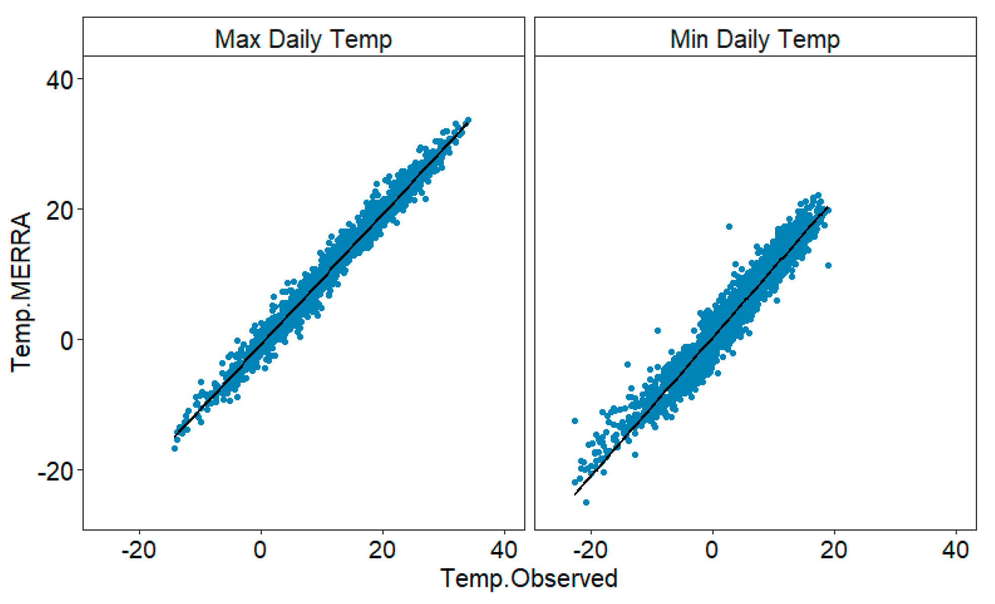
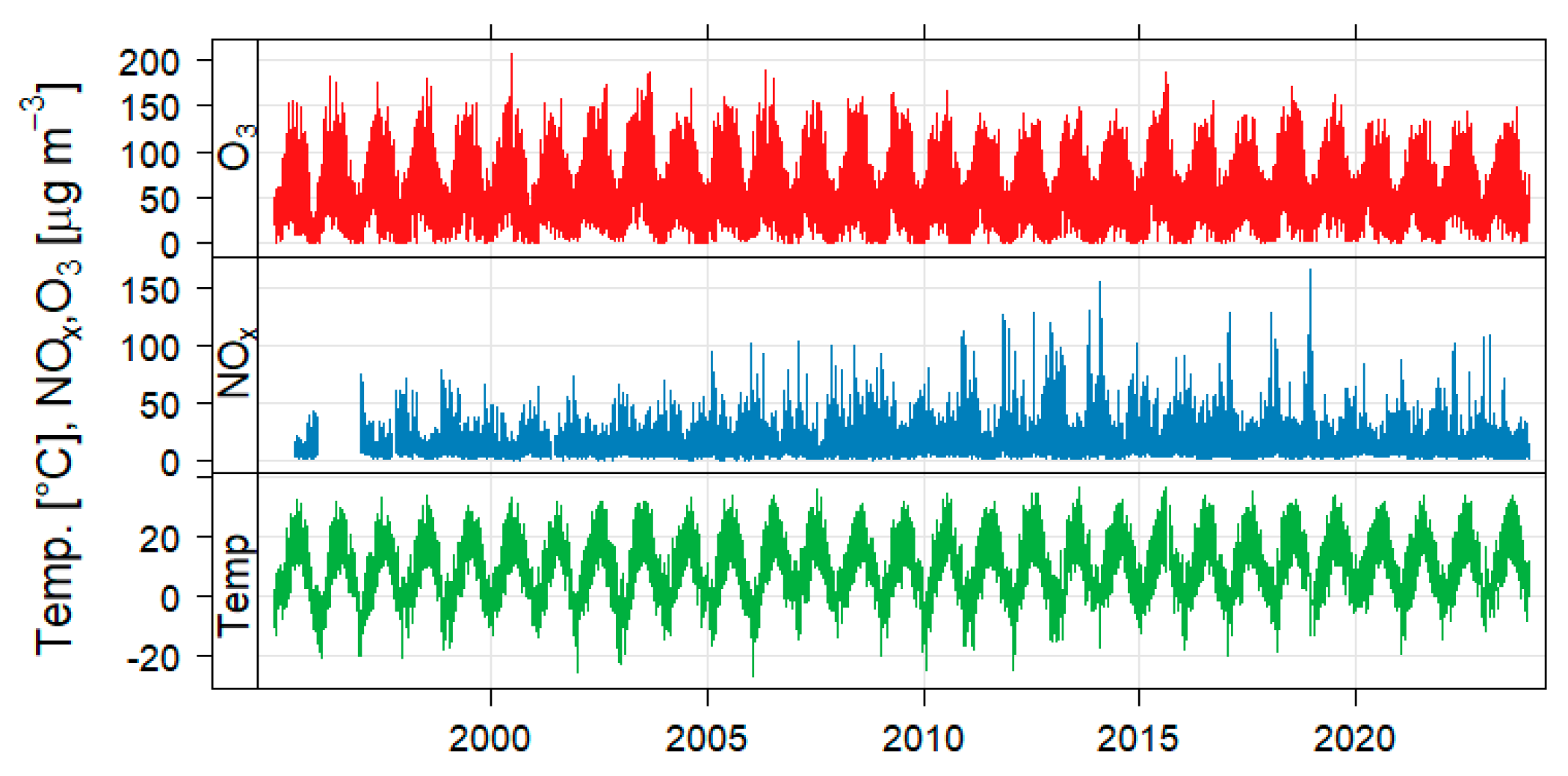
The monitoring of standard trace gasses (O₃, NO, NO₂, SO₂ and CO) in the surface layer of the atmosphere belongs to the broad scientific activity carried out by the main geophysical observatory of the Institute of Geophysics of the Polish Academy of Sciences in Belsk. Considering the station’s surroundings, it falls into the category of background site. Belsk is located in the Mazovian voivodship (central part of Poland), away from industrial zones, congested interregional roads and densely populated areas. The immediate vicinity of the station is dominated by larch forests, orchards and agricultural fields. Consequently, local (up to 1 km from the station) anthropogenic sources of air pollution are typical of rural areas: single-family housing and sparse multi-family housing located along low-traffic municipal roads. The only large city (approx. 50 km to the north) in its vicinity is Warsaw, with 2 million inhabitants. Belsk station has been operating since the early 1990s as a part of the state environmental monitoring coordinated by the Chief Inspectorate of Environmental Protection.

The atmosphere above Belsk was cleared in the 1980s and early 1990s [25] due to the political and economic crisis in Poland, resulting in the collapse of the heavy industry based on coal-fired energy production. Since then, in the post-communist era in Poland, many measures have been taken to protect the environment. However, Poland is still among the countries with the worst air quality in Europe during the heating season [26].

2.2. Data Used

This paper considers the results of O₃ and NO_x measurements in Belsk, i.e., 1 h average concentrations of the gasses in the surface layer of the atmosphere. O₃ data are available from January 1995 to December 2023, while NO_x data are available from July 1995 to December 2023, with a break in 1996. Other shorter data gaps were due to the temporary failures of the measurement equipment.

The air temperature data with a 1 h resolution for the period (1995–2001) were extracted by the Giovanni tool (https://giovanni.gsfc.nasa.gov, accessed on 1 August 2024) from the Modern-ERA Retrospective analysis for Research and Applications, Version 2 (MERRA-2) data base [27], which provided hourly data of the surface air temperature over land with a spatial resolution of 0.5° × 0.625°. We decided to use MERRA-2 temperature for the period of 1995–2001 because there were no hourly resolution temperature measurements at that time. Only the midday temperature and its daily extremes were recorded. This allowed us to verify the MERRA-2 data for the period of 1995–2001. Good agreement was found between the measurements and MERRA-2. Bias and root mean square error of differences between the measurements and MERRA-2 were −0.5 °C and 2.1 °C (for minima), and 0.8 °C and 1.5 °C (for maxima). Figure A1 illustrates the high correlation between measurements and MERRA-2 temperature between 1995 and 2001. From 1 January 2002, temperature measurements with a resolution of 1 h were available. O₃ and NO_x data are in units of [µg/m³], while the air temperature data in units of [°C]. All data are presented in the GMT time format.

The data are divided into the daylight and night subset. Since 1 h averages are collected, for each day, to determine the daylight average of the 24 h data, we start the calculation with a full hour just after sunrise and end with the last full hour just before sunset. The same approach is carried out for the night part of the data, i.e., the start is just after sunset and the end before sunrise. The data are averaged over day, month, season, and year. The following division of the seasons are used: spring (March, April, May), summer (June, July, August), autumn (September, October, November), and winter (December, January, February). Part of the analysis is made based on data taken in the “ozone photochemical season”, i.e., April to September. In addition, the 5th and 95th percentiles, median, and the extreme values for each season and year are analyzed. Cases with less than 75% complete data were excluded from the analyses.

During the period of 1995–2023, the surface O₃ concentrations were monitored by Monitor Labs 8810 (1995–2004), Monitor Labs ME9810 (2004–2014) and Thermo Scientific 49i (2014–2023) analyzers based on the UV absorption method with reference to the norm PN-EN14625. NO_x concentrations were monitored by Monitor Labs 8841 (1995–2004), API 200AU (2004–2014) and Horiba APNA-370 (2014–2023) analyzers based on the chemiluminescence method with reference to the norm PN-EN 14211. All monitors were regularly checked and calibrated with a certified photometer (in the case of surface O₃) and with certified gas mixtures. The ME911 ozone calibrator is certified annually at the Czech Hydrometeorological Institute (CHMI) accredited laboratory in Prague in accordance with National Institute of Standards and Technology (NIST) standard reference photometer (SRP) No. 17. For other trace gasses measured at Belsk, the Thermo 146i calibrator, with certified standard gas mixtures, has been checked at the Central Laboratory of the Central Inspectorate for Environmental Protection in Poland.

3. Results

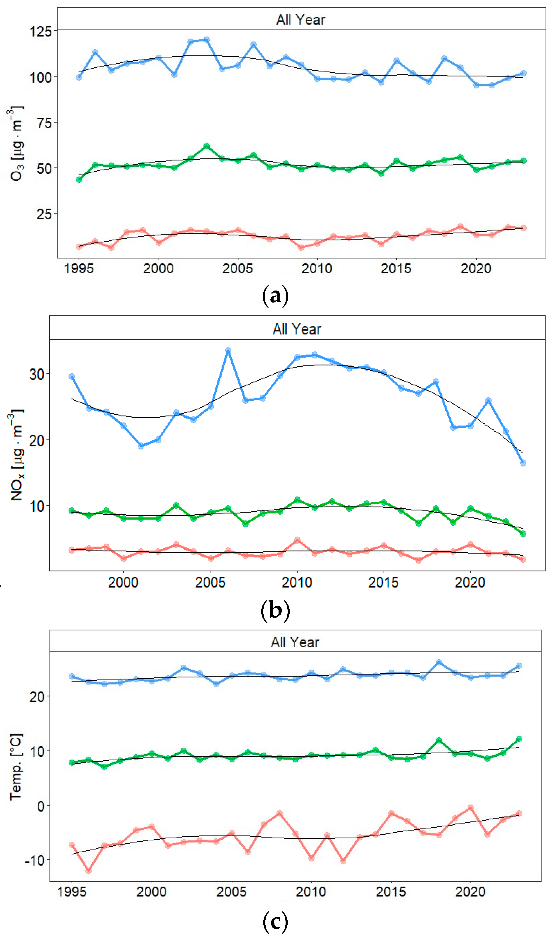
3.1. Trends in Annual and Seasonal Data

This section presents analyses of the annual and seasonal O₃ and NO_x concentrations and air temperature using the following statistical characteristics: 5th, median, and 95th percentiles obtained for each year of observation. The trend results apply to the entire 1995–2023 period and three consecutive subperiods (1995–2004, 2005–2014 and 2015–2023). Figure 1 illustrates the analyzed time series. The seasonality in the data appears especially pronounced in the O₃ and temperature time series.

Table A1. Descriptive statistics from hourly averaged data for O₃, NO_x concentrations and air temperature for the period 1995–2023 and subperiods: 1995–2004, 2005–2014 and 2015–2023. The following abbreviations were used: first quartile (1st Qu), median, mean, third quartile (3rd Qu), 1 h maximum (Max).

	O3 [µg/m3]				NOx [µg/m3]				Temperature [°C]
	1995– 2004	2005– 2014	2015– 2023	1995– 2023	1995– 2004	2005– 2014	2015– 2023	1995– 2023	1995– 2004	2005– 2014	2015– 2023	1995– 2023
	Year				Year				Year
1st Qu	34.0	32.8	35.9	34.0	6.0	5.9	5.2	5.6	0.6	2.1	3.2	1.9
Median	52.0	51.0	52.6	52.0	8.7	9.4	8.3	8.8	8.6	9.1	9.5	9.1
Mean	55.2	53.5	54.6	54.4	10.3	12.0	10.4	11.0	8.3	9.0	10.0	9.0
3rd Qu	73.5	71.3	70.7	71.9	13.0	15.2	13.1	13.8	15.8	15.9	16.6	16.1
Max	208.0	188.9	187.5	208.0	77.6	155.6	165.9	165.9	33.6	36.7	36.4	36.7
	Spring				Spring				Spring
1st Qu	56.0	55.2	54.5	55.2	6.0	5.2	5.1	5.4	2.7	4.1	4.5	3.7
Median	71.5	70.8	68.2	70.0	9.0	8.2	7.7	8.2	8.3	9.0	8.9	8.7
Mean	73.2	72.0	69.1	71.5	10.0	10.1	9.4	9.8	8.3	9.0	9.2	8.8
3rd Qu	89.0	87.4	83.0	86.4	12.6	12.9	11.8	12.4	13.5	13.7	13.7	13.6
Max	182.0	188.9	147.8	188.9	61.4	98.4	101.9	101.9	13.5	32.0	30.2	32.0
	Summer				Summer				Summer
1st Qu	48.3	45.4	46.7	46.9	4.1	4.5	4.0	4.2	15.3	15.3	16.2	15.5
Median	66.6	62.9	63.7	64.4	6.0	6.8	6.4	6.4	18.2	18.4	19.1	18.6
Mean	69.9	65.8	66.7	67.5	7.1	8.2	7.7	7.7	18.6	18.8	19.6	19.0
3rd Qu	89.0	84.0	84.9	86.0	9.0	10.3	9.9	9.8	21.6	22.0	22.7	22.1
Max	208.0	180.6	187.5	208.0	42.0	128.6	76.0	128.6	33.6	36.7	36.4	36.7
St. Dev.	29.0	27.3	26.7	27.7	4.1	5.6	5.3	5.1	4.5	4.9	4.8	4.8
	Autumn				Autumn				Autumn
1st Qu	23.0	20.5	24.7	22.8	6.0	7.2	5.9	6.4	3.7	5.1	6.1	4.9
Median	37.0	34.2	38.0	36.3	9.0	11.3	9.1	9.8	8.5	9.0	9.8	9.1
Mean	39.0	36.5	40.5	38.6	10.5	13.8	11.2	11.9	8.3	9.2	10.1	9.1
3rd Qu	51.1	49.9	52.7	51.3	13.0	17.3	14.0	14.8	12.8	13.1	14.0	13.2
Max	171.0	140.6	173.6	173.6	77.6	130.1	108.2	130.1	29.2	30.4	30.3	30.4
	Winter				Winter				Winter
1st Qu	23.0	25.1	28.5	25.4	7.5	7.8	6.6	7.2	−5.7	−4.2	−1.4	−4.0
Median	38.0	39.3	42.6	40.0	11.0	12.8	10.7	11.5	−1.7	−0.2	1.0	−0.2
Mean	38.6	39.4	41.9	39.9	13.3	16.1	13.3	14.3	−2.5	−1.1	0.9	−1.0
3rd Qu	52.3	53.0	55.6	53.8	16.5	20.8	17.0	18.0	1.1	2.8	3.9	2.6
Max	134.3	120.9	101.6	134.3	75.2	155.6	165.9	165.9	14.0	14.1	16.8	16.8

shows the corresponding descriptive statistics for these time series. The warming of the surface layer can be inferred for all seasons and in the annual data, as most statistics show a gradual increase in temperature in three consecutive subsets of the data. The direction of changes in the gas components is not so clear, and often the lowest or highest value in the three subsets appeared for the middle subset of the data. To assess the significance of such changes, linear trends in the time series of the 5th, median and 95th percentile were calculated.

3.1.1. O₃ Time Series

Figure 2a (annual data) and Figure A2a (seasonal data) show the time series used in the trend calculations. A locally weighted scatter smoothing (Lowess) was applied to these series to illustrate the long-term variability in these series [28]. In general, three phases in the smoothed 1995–2023 pattern can be identified: an increase at the beginning, then a decrease in the middle of the time series, and a leveling off at the end. The entire time series appears to be trendless.

Trend analyses using standard least squares linear regression confirm these three phases of the long-term O₃ changes, but statistically significant (at the 2σ level) linear trends occur in 20 cases out of a total of 60 cases. Namely, in the 1995–2004 period, positive trends are identified for the 5th percentile (1.37 ± 0.56 µg/m³/y in the summer), for the median (0.94 ± 0.32 µg/m³/y in the autumn, and 1.48 ± 0.58 µg/m³/y in the winter), and for the 95th percentile (2.11 ± 0.74 µg/m³/y in the winter). In the 2005–2014 period, a negative trend is revealed for the 5th percentile (−0.77 ± 0.34 µg/m³/y in the summer), for the median (−1.34 ± 0.53 µg/m³/y in the summer, and −0.89 ± 0.34 µg/m³/y in the autumn), and for the 95th percentile (−1.78 ± 0.68 µg/m³/y in the spring, and −2.14 ± 0.90 µg/m³/y in the summer). In the period of 2015–2023, only one statistically significant trend is found for the 5th percentile (0.44 ± 0.14 µg/m³/y in the autumn). For the year-round data, the positive trends appear in the 1995–2004 period for the 5th percentile (0.85 ± 0.33 µg/m³/y), and for the median (1.16 ± 0.36 µg/m³/y), whereas negative trends are revealed in the 2005–2014 period for the median (−0.70 ± 0.23 µg/m³/y) and the 95th percentile (−1.65 ± 0.49 µg/m³/y). There were no statistically significant trends in the last 2015–2023 period.

Over the entire period of measurements (1995–2023), statistically significant positive trends are found in the year-round data for the 5th percentile (0.15 ± 0.07 µg/m³/y), and a negative trend for the 95th percentile (−0.38 ± 0.14 µg/m³/y). In addition, statistically significant seasonal trends were identified, i.e., positive for the 5th percentile (0.20 ± 0.07 µg/m³/y in the winter) and for the median (0.28 ± 0.08 µg/m³/y in the winter), and a negative trend for the 95th percentile (−0.44 ± 0.15 µg/m³/y in the spring, and −0.50 ± 0.21 µg/m³/y in the summer).

3.1.2. NO_x Time Series

The annual (Figure 2b) and seasonal (Figure A2b) changes in NO_x concentrations between 1995 and 2023 have been analyzed in a similar way to O₃ concentrations (Section 3.1.1). The existence of opposite trends in consecutive parts of the series can be inferred from the smoothed pattern of NO_x changes.

Trend analyses by standard least squares linear regression provided statistically significant values only in several cases out of a total of 60 cases. These are as follows: the positive trends in 2005–2014 for the median (0.48 ± 0.12 µg/m³/y in the winter) and the negative trends in the period of 2015−2023 for the median (−0.20 ± 0.08 µg/m³/y in the summer, and −0.55 ± 0.18 µg/m³/y in the autumn), and for the 95th percentile (−1.94 ± 0.44 µg/m³/y in the autumn, and −1.36 ± 0.53 µg/m³/y in the winter). Moreover, for the year-round data, the two negative trends are found in the 2015–2023 period for the median values (−0.37 ± 0.15 µg/m³/y) and the 95th percentile (−1.39 ± 0.31 µg/m³/y).

3.1.3. Air Temperature Time Series

Figure 2c and Figure A2c show annual and seasonal variations in surface temperature, respectively. The same approach as in the previous two subsections was applied to discuss long-term changes in the 5th percentile, the median, and the 95th percentile over 1995–2023. The patterns of the smoothed time series of temperature suggest a slight upward trend in the annual and seasonal data.

Statistically significant positive trends were revealed for the entire period of 1995–2023 in the summer and annual time series for all considered statistics. The summer trends are (0.03 ± 0.01 °C/y), (0.04 ± 0.01 °C/y), and (0.08 ± 0.02 °C/y) for the 5th percentile, median, and the 95th percentile, respectively. The winter trends are (0.18 ± 0.08 °C/y), (0.15 ± 0.04 °C/y), and (0.15 ± 0.04 °C/y) for the 5th percentile, median, and the 95th percentile, respectively. The year-round trends are (0.18 ± 0.05 °C/y), (0.07 ± 0.02 °C/y), and (0.06 ± 0.02 °C/y), respectively. Moreover, statistically significant positive trends were found for the 5th percentile in the autumn (0.15 ± 0.04 °C/y) and for median (0.05 ± 0.02 °C/y in the spring, and 0.08 ± 0.02 °C/y in autumn).

3.1.4. Trends in Monthly and Hourly Extremes

In this section, we focus on the long-term changes in the monthly and hourly extremes obtained for each year in the period of 1995–2023. Both minima and maxima are considered. We used the standard least squares fit to calculate the trends and their standard errors.

Figure 3a shows that the monthly and hourly maxima decreased but the monthly minima increased in the analyzed period. The regression lines have the following statistically significant slopes, 0.26 ± 0.09 µg/m³/y for monthly minima, −0.25 ± 0.14 µg/m³/y for monthly maxima (p-value of 0.08), and −1.16 ± 0.30 µg/m³/y for 1 h maxima.

Figure 3b presents the long-term variability in the monthly NO_x maxima and minima and 1 h maxima during the year. The 1995−2023 trends in the monthly NO_x maxima and minima appeared statistically insignificant. In case of 1 h maxima, a statistically significant positive trend (1.93 ± 0.67 µg/m³/y) was found.

Figure 3c shows the long-term variability in the monthly temperature minima and maxima, and 1 h maxima during the year. Statistically significant positive trends were found for monthly minima (0.19 ± 0.05 °C/y) confirming the warming of the surface atmosphere over Belsk. Almost statistically significant trends of 0.06 ± 0.03 °C/y were calculated for the monthly maxima and 1 h temperature maxima during the year, respectively.

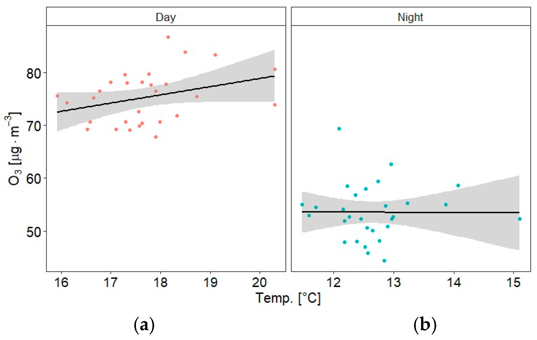
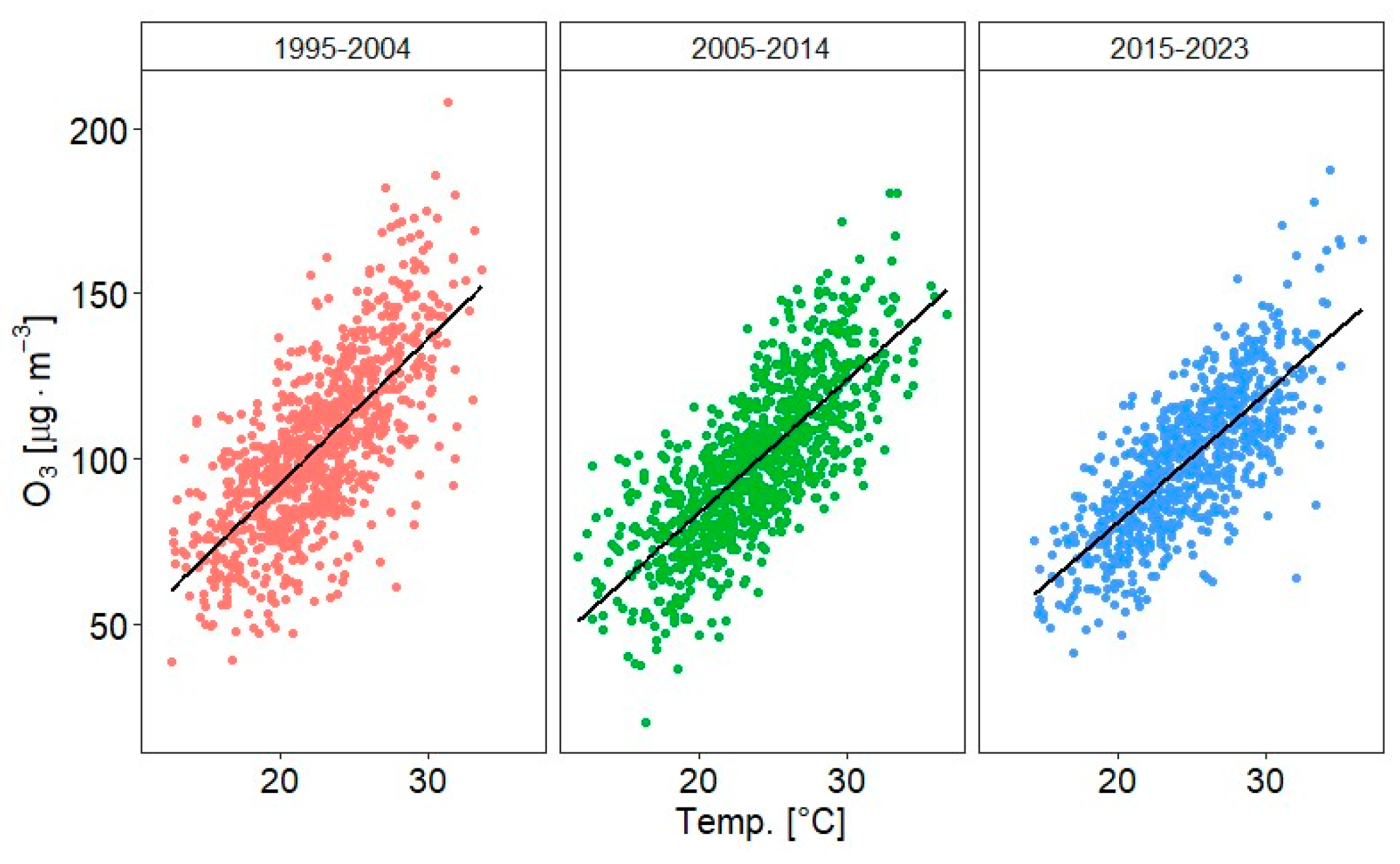
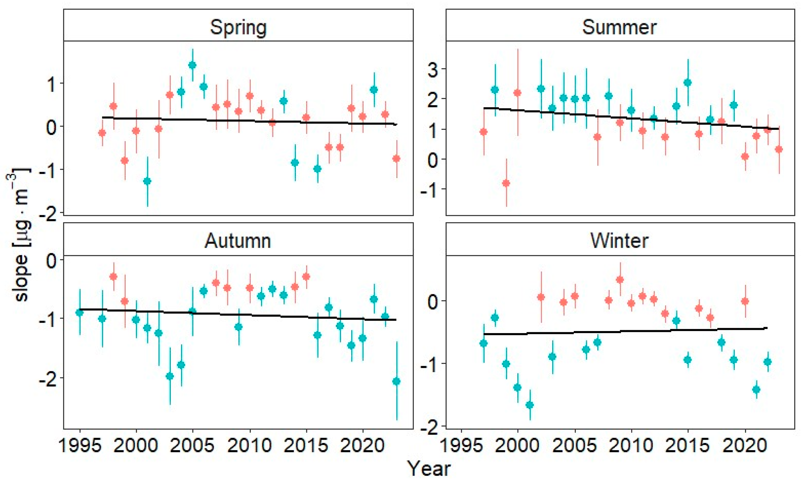
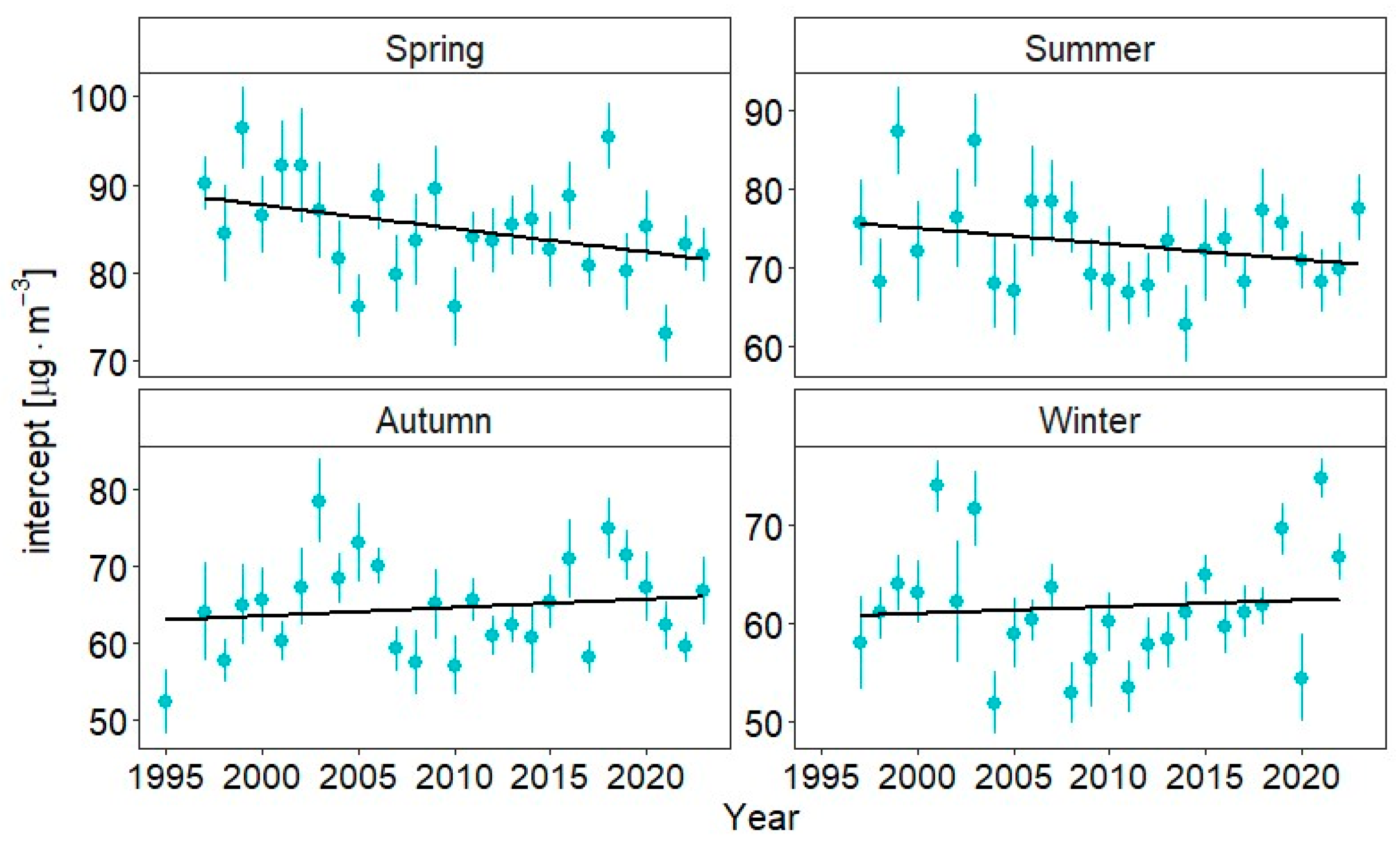
3.2. Relationship between Surface O₃ and Air Temperature

The chemical processes leading to the formation of O₃ vary nonlinearly with temperature [29]. An increase in the temperature increases the rate of chemical reactions, as well as enhancing the evaporative and biogenic VOC emission [9].

The O₃ concentrations measured during daylight (sunrise–sunset) and averaged from April to September versus the corresponding temperature are shown in Figure 4a for each year in the 1995–2023 period. This part of the year, i.e., the photochemical O₃ production season, is characterized by a high potential of photochemical O₃ build-up, and O₃ concentrations sometimes exceed the permitted threshold of 120 µg/m³ for the daily maximum 8 h O₃ running mean. The processes of effective O₃ production result from favorable meteorological conditions (high temperature, intensive solar radiation) as well as the availability of the surface O₃ precursors (organic emission of VOCs). Correspondingly, Figure 4b shows the O₃–temperature pairs calculated for the night period.

The average O₃ concentrations for the daylight period ranged between 67.9 and 86.8 µg/m³ and temperature varied between 15.9 and 20.3 °C, while during night the corresponding ranges were 44.4–69.4 µg/m³ and 11.5–15.1 °C. An increase in the daylight O₃ with temperature can be estimated from the slope of the regression line shown in Figure 4a. For the night data (Figure 4b), O₃ changes appeared to be independent of the temperature. A weak (but statistically significant) correlation coefficient of 0.33 was calculated for the daylight period, while the correlation coefficient was −0.01 for the night data. The increasing rate of 1.56 ± 0.87 µg/m³/°C (p-value of 0.08) and −0.04 ± 1.37 µg/m³/°C (p-value of 0.98) was obtained from the slopes of the regression line for the daylight and night data, respectively.

Figure 5 shows the annual time series of maximum O₃ concentrations found when the temperature was within the selected intervals of 1 °C width. The intervals were from 24.5–25.5 °C up to 32.5–33.5 °C. Negative trends in the O₃ maxima can be guessed from the slopes of the regression line fitted to the maxima variations in 1995–2025. For more than half of the intervals, i.e., 25, 26, 27, 28, 29 and 33 °C ± 0.5 °C, the negative trends were statistically significant with the rate of −1.0 ± 0.2 µg/m³/y, −1.1 ± 0.2 µg/m³/y, −1.5 ± 0.3 µg/m³/y, −1.5 ± 0.4 µg/m³/y, −1.0 ± 0.4 µg/m³/y and −1.5 ± 0.7 µg/m³/y, respectively.

The highest 1 h O₃ concentration (208 µg/m³) was found in 2000 at the temperature of 28 °C. The concentrations above 180 µg/m³ (i.e., the so-called the “information” threshold) were noted at 34 °C (2015), 31 °C (2000), 30 °C (2000, 2003), 29 °C (2000, 2003, 2006), 28 °C (2000, 2006), 27 °C (2000, 2003) as well as at 22 °C (1996) and at 21 °C (2000).

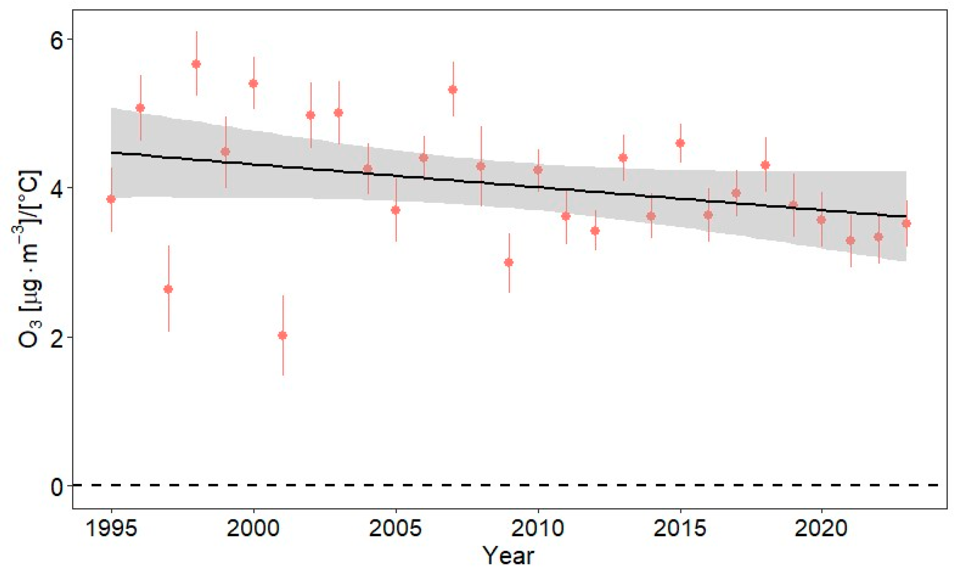
3.3. Ozone–Climate Penalty

The ozone–climate penalty factor, m _O3−T, is defined here as the value of the slope of linear regression of the daily 1 h O₃ maxima on the corresponding temperature maxima. The calculations of m _O3−T values were performed for summer season (June, July, August) for three consecutive periods: 1995–2004, 2005–2014, and 2015–2023. For these periods, Figure 6 shows scatterplots of the daily O₃ maxima versus temperature maxima, along with a linear regression to estimate m _O3−T value (the slope of the line). The highest m _O3−T value of 4.40 µg/m³/°C was found in the first period (1995–2004). For the next period, m _O3−T value was lower (4.04 µg/m³/°C), and the smallest one of 3.93 µg/m³/°C was found in the last period. The steady decrease in these decadal m _O3−T values suggests a downward trend in m _O3−T values throughout the entire observation period. This is confirmed by the negative trend equal to −0.031 ± 0.018 µg/m³/°C/y (p-value of 0.10) found in the annual time series of m _O3−T from 1995 to 2023 (Figure 7).

3.4. Photochemical O_x Production Regime

Figure 8 shows an example of a scatter plot of the daylight means of O_x concentration versus the daylight means of NO_x concentration for all seasons in 1998. The analysis of such a plot allows us to delineate “local” and “regional” contribution to O_x variability, and provides the photochemical O_x production regime at the observing site: “NO_x-limited” or “VOC-limited”. The value of the slope of the linear regression fitted to O_x-NO_x pairs determines a magnitude of the “local” contribution to O₃ variability. The negative value of the slope means an increase (decrease) of O_x concentration with decreasing (increasing) NO_x concentration (regime: “VOC-limited”, see autumn and winter in Figure 8) while the positive slope is for an increase (decrease) of O_x concentration with increasing (decreasing) NO_x concentration (regime: “NO_x—limited”, see spring and summer in Figure 8). The intercept of the linear regression indicates a magnitude of the regional O_x contribution.

Figure 9 shows the time series of the magnitude “local” contribution to O₃ variability in the four seasons for each year from 1995 to 2023. The photochemical regime of the O_x variability exhibited large fluctuations in that period. In the summer, the “NO_x-limited” regime was found in 13 years (i.e., in years when the positive O_x-NO_x slope was statistically significant) out of a total of 29 years, whereas in spring it was identified only in 5 years. The “VOCs-limited “regime appeared in 22 and 14 years in autumn and winter, respectively. In addition, there were three such cases in spring. For each season, there was no statistically significant trend in the time series of the magnitude of the “local” contribution to O_x variability over the period of 1995–2023. The type of regime could not be determined in the last four summer seasons and the “NO_x-limited” regime occurred mainly in the first half of the 1995–2023 period.

The time series of “regional” contribution to seasonal O_x variations are shown in Figure 10. The trends in “regional” contributions were found to be statistically insignificant for all seasons in the 1995–2023 period. The regional sources showed clear seasonality with a springtime maximum and a winter minimum characteristic for background surface O₃ concentration in the Northern Hemisphere [30].

4. Discussion

Reductions in the anthropogenic emissions of surface O₃ precursors over Europe in recent decades have been effective in reducing peak O₃ concentrations, but the task of reducing surface O₃ concentrations in other positional statistics is still important [14,17,31]. A decreasing trend in maxima combined with an increasing trend in the minima of the surface O₃ concentration indicated a change in the O₃ distribution [17]. This paper presents similar results to those mentioned above.

Three phases of the long-term variability of O₃ variability can be identified in the rural areas of Central Poland over the period of (1995–2023): an increase at the beginning, a decrease in the middle part of the time series, and a leveling off at the end. Throughout the measurement period, there was a statistically significant positive trend (0.15 ± 0.07 µg/m³/y) at the 5th percentile and a statistically significant negative trend (−0.38 ± 0.14 µg/m³/y) at the 95th percentile. Analyzing the seasonal O₃ variations, a negative trend was observed in spring (−0.44 ± 0.15 µg/m³/y) and summer (−0.50 ± 0.21 µg/m³/y) at the 95th percentile, and a positive trend in winter at the 5th and median of 0.20 ± 0.07 µg/m³/y and 0.28 ± 0.08 µg/m³/y, respectively.

According to Dentener et al. [32], the decline in the summertime O₃ peaks resulted from the global reduction in the emission of O₃ precursors. Moreover, discrepancies in the decrease in extreme and increase in background surface O₃ concentrations may be determined by meteorological variability and changes in the hemispheric transport of pollution, as well as the enhanced contribution of the lowermost stratospheric O₃ amounts [33].

The emission of NO_x in Europe during the last decades (since 2000) has declined significantly, with an annual reduction of about 2.5%/y [34]. Our results showed two phases of NO_x concentrations during the 1995–2023 period: an increasing tendency towards the middle part of the series (2005–2014), and afterwards (2015–2023) an apparent decreasing tendency can be identified. Many negative trends were noted in the last subperiod (2015–2023) in summer, autumn and winter at the 50th and 95th percentiles. A similar declining tendency in NO_x was noted at rural locations in Germany during 1999–2008 [29]. At the 95th percentile, the NO_x concentrations significantly decreased with a rate of −1.77 µg/m³/y; for comparison, the Belsk rate was −1.39 ±0.31 µg/m³/y at the 95th percentile later on in the 2015–2023 period.

The trend analyses of the surface temperature at Belsk supported continuous atmosphere warming, with the approximate rate of 0.05–0.10 °C/y. We found a corresponding increase in the average O₃ level in daylight during the photochemical season (April–September) in contrast to the night hours, when there was no relationship between O₃ and temperature. However, the annual maxima of O₃ concentration show a statistically significant declining tendency over the entire period of the measurements. In addition, a statistically significant declining tendency appeared in the time series of O₃ maxima for many fixed temperature intervals of 1 °C, from 25 °C to 33 °C. This means that O₃ accumulation at high temperatures was slowed down during very warm days because less NO₂ was available for photolysis. Therefore, photochemical smog has become a very rare phenomenon in Belsk.

In accordance to the European Union Air Quality Directive 2008/50/EC of 21 May 2008 [35], we currently have four target O₃ values for the protection of human health: the alarm threshold (1 h O₃ > 240 µg/m³), the information threshold (1 h O₃ > 180 µg/m³), the target level threshold (the maximum 8 h O₃ > 120 µg/m³ exceeded 25 days at most, averaged over the following three years) and the long-term threshold level (maximum 8 h O₃ > 120 µg/m³). The alarm threshold at Belsk was never exceeded during the 1995–2023 period, and the highest O₃ concentration was equal to 208 µg/m³ (21 June 2000). The O₃ alarm threshold value for informing the public about the risk of occurrence was noted 17 times, in April 1996, in June 2000, in August 2003, in May and July 2006 and in August 2015. The longest episode of surface O₃ concentrations > 180 µg/m³ lasted 6 h, and was noted on 21 June 2000 from 8 a.m. to 13 p.m. Almost all cases were noted in the first half of measurement period and only one exceedance of information threshold was noted during the second half of measurement (2015). Exceedances of the target level threshold were noted every year between 2002 and 2008, with the exception of 2006. Similar to the information threshold, exceedances of the target level threshold were recorded only in the first half of the measurement period.

The long-term variations in the ozone–climate penalty factor, m _O3−T, indicated its steady decrease over the 1995–2023 period. The highest value is found in the first period (1995–2004) equal to 4.4 µg/m³/C and the lowest for the last period (2015–2023), with a value of 3.9 µg/m³/C. These values are comparable to the m _O3−T values (4.0–5.0 µg/m³/C) observed at the rural stations located in eastern and northern Germany over 1999–2018 [29]. A decrease in m _O3−T was found for the long-term data across different locations: rural, urban and suburban, with the higher m _O3−T value for the period of (1999–2008) compared to the period of 2009–2018. Similar results were obtained by Boleti et al. [36]. For most of the regions in Europe (with the exception of the northern part) significant downward trends in m _O3−T of approximately 0.04–0.05 ppb/°C/y were revealed. Moreover, the negative trend in m _O3−T was larger in highly and moderately polluted areas. There was also a downward trend in m _O3−T at Belsk, but several times smaller, i.e., 0.017 ± 0.009 ppb/°C/y for the period 1995–2023.

The method of linear regression of oxidants (O_x) against NO_x concentrations was used to estimate local (NO_x-dependent) and regional (NO_x-independent) contributions to O_x, as well as indicate the dominant photochemical regime (“NO_x-limited” or “VOC-limited”). There was a greater likelihood of the “NO_x-limited” regime in the summer and “VOC-limited” regime in the autumn–winter. In the period of 1995–2023, the “VOC-limited” regime was never found in the summer and, vice versa, the “NO_x-limited” regime was absent in the winter and autumn. For many seasons, the regime type could not be identified. This means that it is difficult to build an effective national policy to improve the air quality, because the type of the photochemical regime is so variable in rural areas of Poland.

5. Conclusions

• O₃ trends depend on the period studied, as well as the season and the selected statistical characteristics (95th and 5th percentile, median, 1 h and monthly extremes). Trends may even be opposite in two consecutive sub-periods (e.g., 95th percentile for summer in 1995–2004 and 2005–2014). Therefore, when comparing trends between stations, always consider the same period, season and statistical characteristics.
• The lack of seasonal trends in local and regional contributions to O₃ variability has stabilized the average O₃ level in Belsk since 1995.
• Currently, the appearance of photochemical smog in Belsk is very unlikely.
• Average O₃ levels will increase with global warming, but the reduction in the ozone–climate penalty factor observed at many sites, including Belsk, suggests that any estimate of future average O₃ levels should be treated with caution.

References

1. Intergovernmental Panel on Climate Change (IPCC). Climate Change 2022—Impacts, Adaptation and Vulnerability; Cambridge University Press: Cambridge, UK, 2023. [Google Scholar]
2. Lelieveld, J.; Evans, J.S.; Fnais, M.; Giannadaki, D.; Pozzer, A. The Contribution of Outdoor Air Pollution Sources to Premature Mortality on a Global Scale. Nature 2015, 525, 367–371. [Google Scholar] [CrossRef] [PubMed]
3. Lelieveld, J.; Dentener, F.J. What Controls Tropospheric Ozone? J. Geophys. Res. Atmos. 2000, 105, 3531–3551. [Google Scholar] [CrossRef]
4. Jiang, W.; Singleton, D.L.; Hedley, M.; Mclaren, R. Sensitivity of Ozone concentrations to VOC and NOx Emissions in the Canadian Lower Fraser Valley. Atmos. Environ. 1997, 31, 627–638. [Google Scholar] [CrossRef]
5. Sillman, S. Chapter 12 The Relation between Ozone, NOx and Hydrocarbons in Urban and Polluted Rural Environments. In Developments in Environmental Science; Elsevier: Amsterdam, The Netherlands, 2002; Volume 1. [Google Scholar] [CrossRef]
6. Li, M.; Karu, E.; Brenninkmeijer, C.; Fischer, H.; Lelieveld, J.; Williams, J. Tropospheric OH and Stratospheric OH and Cl Concentrations Determined from CH4, CH3Cl, and SF6 Measurements. NPJ Clim. Atmos. Sci. 2018, 1, 29. [Google Scholar] [CrossRef]
7. Flowerday, C.E.; Thalman, R.; Hansen, J.C. Local and Regional Contributions to Tropospheric Ozone Concentrations. Atmosphere 2023, 14, 1262. [Google Scholar] [CrossRef]
8. Sillman, S.; He, D. Some Theoretical Results Concerning O3-NOx-VOC Chemistry and NOx-VOC Indicators. J. Geophys. Res. Atmos. 2002, 107, ACH 26-1–ACH 26-15. [Google Scholar] [CrossRef]
9. Pusede, S.E.; Steiner, A.L.; Cohen, R.C. Temperature and Recent Trends in the Chemistry of Continental Surface Ozone. Chem. Rev. 2015, 115, 3898–3918. [Google Scholar] [CrossRef]
10. Abeleira, A.J.; Farmer, D.K. Summer Ozone in the Northern Front Range Metropolitan Area: Weekend-Weekday Effects, Temperature Dependences, and the Impact of Drought. Atmos. Chem. Phys. 2017, 17, 6517–6529. [Google Scholar] [CrossRef]
11. Leighton, P.A. Photochemistry of Air Pollution; Academic Press: New York, NY, USA, 1961. [Google Scholar]
12. Clapp, L.J.; Jenkin, M.E. Analysis of the Relationship between Ambient Levels of O3, NO2 and NO as a Function of NOx in the UK. Atmos. Environ. 2001, 35, 6391–6405. [Google Scholar] [CrossRef]
13. Derwent, R.G.; Hjellbrekke, A.-G. Air Pollution by Ozone Across Europe. In Urban Air Quality in Europe; Springer: Berlin/Heidelberg, Germany, 2012; pp. 55–73. [Google Scholar]
14. Yan, Y.; Lin, J.; Pozzer, A.; Kong, S.; Lelieveld, J. Trend Reversal from High-to-Low and from Rural-to-Urban Ozone Concentrations over Europe. Atmos. Environ. 2019, 213, 25–36. [Google Scholar] [CrossRef]
15. Guerreiro, C.B.B.; Foltescu, V.; de Leeuw, F. Air Quality Status and Trends in Europe. Atmos. Environ. 2014, 98, 376–384. [Google Scholar] [CrossRef]
16. Querol, X.; Alastuey, A.; Reche, C.; Orio, A.; Pallares, M.; Reina, F.; Dieguez, J.J.; Mantilla, E.; Escudero, M.; Alonso, L.; et al. On the Origin of the Highest Ozone Episodes in Spain. Sci. Total Environ. 2016, 572, 379–389. [Google Scholar] [CrossRef] [PubMed]
17. Colette, A.; Andersson, C.; Manders, A.; Mar, K.; Mircea, M.; Pay, M.T.; Raffort, V.; Tsyro, S.; Cuvelier, C.; Adani, M.; et al. EURODELTA-Trends, a Multi-Model Experiment of Air Quality Hindcast in Europe over 1990–2010. Geosci. Model Dev. 2017, 10, 3255–3276. [Google Scholar] [CrossRef]
18. Atkinson, R. Gas-Phase Tropospheric Chemistry of Organic Compounds: A Review. Atmos. Environ. Part A Gen. Top. 1990, 24, 1–41. [Google Scholar] [CrossRef]
19. Guenther, A.; Karl, T.; Harley, P.; Wiedinmyer, C.; Palmer, P.I.; Geron, C. Estimates of Global Terrestrial Isoprene Emissions Using MEGAN (Model of Emissions of Gases and Aerosols from Nature). Atmos. Chem. Phys. 2006, 6, 3181–3210. [Google Scholar] [CrossRef]
20. Roberts, J.M.; Bertman, S.B. The Thermal Decomposition of Peroxyacetic Nitric Anhydride (PAN) and Peroxymethacrylic Nitric Anhydride (MPAN). Int. J. Chem. Kinet. 1992, 24, 297–307. [Google Scholar] [CrossRef]
21. Weng, H.; Lin, J.; Martin, R.; Millet, D.B.; Jaeglé, L.; Ridley, D.; Keller, C.; Li, C.; Du, M.; Meng, J. Global High-Resolution Emissions of Soil NOx, Sea Salt Aerosols, and Biogenic Volatile Organic Compounds. Sci. Data 2020, 7, 148. [Google Scholar] [CrossRef] [PubMed]
22. Bloomer, B.J.; Stehr, J.W.; Piety, C.A.; Salawitch, R.J.; Dickerson, R.R. Observed Relationships of Ozone Air Pollution with Temperature and Emissions. Geophys. Res. Lett. 2009, 36, L09803. [Google Scholar] [CrossRef]
23. Brown, F.; Folberth, G.A.; Sitch, S.; Bauer, S.; Bauters, M.; Boeckx, P.; Cheesman, A.W.; Deushi, M.; Dos Santos Vieira, I.; Galy-Lacaux, C.; et al. The Ozone-Climate Penalty over South America and Africa by 2100. Atmos. Chem. Phys. 2022, 22, 12331–12352. [Google Scholar] [CrossRef]
24. Zanis, P.; Akritidis, D.; Turnock, S.; Naik, V.; Szopa, S.; Georgoulias, A.K.; Bauer, S.E.; Deushi, M.; Horowitz, L.W.; Keeble, J.; et al. Climate Change Penalty and Benefit on Surface Ozone: A Global Perspective Based on CMIP6 Earth System Models. Environ. Res. Lett. 2022, 17, 024014. [Google Scholar] [CrossRef]
25. Posyniak, M.; Szkop, A.; Pietruczuk, A.; Podgórski, J.; Krzyścin, J. The Long-Term (1964–2014) Variability of Aerosol Optical Thickness and Its Impact on Solar Irradiance Based on the Data Taken at Belsk, Poland. Acta Geophys. 2016, 64, 1858–1874. [Google Scholar] [CrossRef]
26. De Brito, C.; Guerreiro, B.; Profile, S.; González Ortiz, A. Air Quality 2018—EEA Report 12 2018. Available online: https://op.europa.eu/en/publication-detail/-/publication/223e663b-1340-11e9-81b4-01aa75ed71a1/language-en (accessed on 1 August 2024). [CrossRef]
27. Global Modeling and Assimilation Office (GMAO). MERRA-2 Inst1_2d_lfo_Nx: 2d,1-Hourly, Instantaneous, Single-Level, Assimilation, Land Surface Forcings V5.12.4, Greenbelt, MD, USA, Goddard Space Flight Center Distributed Active Archive Center (GSFC DAAC). 2015. Available online: https://disc.gsfc.nasa.gov/datasets/M2I1NXLFO_5.12.4/summary (accessed on 28 May 2024). [CrossRef]
28. Cleveland, W.S. Robust Locally Weighted Regression and Smoothing Scatterplots. J. Am. Stat. Assoc. 1979, 74, 829–836. [Google Scholar] [CrossRef]
29. Otero, N.; Rust, H.W.; Butler, T. Temperature Dependence of Tropospheric Ozone under NOx Reductions over Germany. Atmos. Environ. 2021, 253, 118334. [Google Scholar] [CrossRef]
30. Monks, P.S. A Review of the Observations and Origins of the Spring Ozone Maximum. Atmos. Environ. 2000, 34, 3545–3561. [Google Scholar] [CrossRef]
31. Wilson, R.C.; Fleming, Z.L.; Monks, P.S.; Clain, G.; Henne, S.; Konovalov, I.B.; Szopa, S.; Menut, L. Have Primary Emission Reduction Measures Reduced Ozone across Europe? An Analysis of European Rural Background Ozone Trends 1996–2005. Atmos. Chem. Phys. 2012, 12, 437–454. [Google Scholar] [CrossRef]
32. Dentener, F.; Keating, T.; Akimoto, H. Convention on Long-range Transboundary Air Pollution. Task Force on Hemispheric Transport of Air Pollution. In Hemispheric Transport of Air Pollution 2010. Part A, Ozone and Particulate Matter; United Nations. Economic Commission for Europe: Geneva, The Netherlands, 2010. [Google Scholar]
33. Ordóñez, C.; Brunner, D.; Staehelin, J.; Hadjinicolaou, P.; Pyle, J.A.; Jonas, M.; Wernli, H.; Prévot, A.S.H. Strong Influence of Lowermost Stratospheric Ozone on Lower Tropospheric Background Ozone Changes over Europe. Geophys. Res. Lett. 2007, 34, L07805. [Google Scholar] [CrossRef]
34. Aas, W.; Fagerli, H.; Alastuey, A.; Cavalli, F.; Degorska, A.; Feigenspan, S.; Brenna, H.; Gliß, J.; Heinesen, D.; Hueglin, C.; et al. Trends in Air Pollution in Europe, 2000–2019. Aerosol Air Qual. Res. 2024, 24, 230237. [Google Scholar] [CrossRef]
35. Directive 2008/50/EC of the European Parliament and of the Council of 21 May 2008 on Ambient Air Quality and Cleaner Air for Europe. Available online: https://www.eea.europa.eu/policy-documents/directive-2008-50-ec-of (accessed on 31 July 2024).
36. Boleti, E.; Hueglin, C.K.; Grange, S.; Takahama, S. Temporal and Spatial Analysis of Ozone Concentrations in Europe Based on Timescale Decomposition and a Multi-Clustering Approach. Atmos. Chem. Phys. 2020, 20, 9051–9066. [Google Scholar] [CrossRef]
Figure 1. Time series (1995–2023) of hourly averaged surface O3 [µg/m3] (top), NOx [µg/m3] (middle) and air temperature [°C], (bottom panel).
Atmosphere 15 00960 g001
Figure 2. The 5th percentile (red), median (green) and 95th percentile (blue) percentile for each year during the 1995–2023 period: (a) O3 data; (b) NOx data; (c) temperature data. The black curve indicates the smoothed pattern by the Lowess smoother.
Atmosphere 15 00960 g002
Figure 3. Time series of monthly extremes (monthly minimum-blue, monthly maximum-green) and hourly maximum (red) in each year during the period of 1995–2023: (a) O3 data; (b) NOx data; (c) temperature data. Lines are from standard least squares regression.
Atmosphere 15 00960 g003
Figure 4. O3 concentrations averaged over the April–September period for each year in the 1995–2023 periods versus corresponding averaged temperature (points): (a) the daylight (sunrise–sunset) part of the data; (b) the night (sunset–sunrise) part of the data. The black solid line represents the linear regression and the gray area provides the 95% confidence interval for the fit.
Atmosphere 15 00960 g004
Figure 5. Maximum O3 concentrations found in each year (from 1995 up to 2023) when temperature was within the selected interval of 1 °C (points). The intervals were set from 25 °C to 33 °C ± 0.5 °C. The black line indicates the linear regression. Statistically significant trends are marked in blue while statistically insignificant trends are indicated in red.
Atmosphere 15 00960 g005
Figure 6. Scatter plot of daily O3 maximum versus corresponding temperature maximum for three consecutive periods (points): 1995–2004, 2005–2014 and 2015–2023. The black line indicates a linear regression. The slope of this line provides the value of the ozone–climate penalty.
Atmosphere 15 00960 g006
Figure 7. Time series of the annual values of ozone–climate penalty factor calculated for each year in the 1995–2023 period. The vertical bars indicate the standard deviations of the annual value of ozone–climate penalty factor.
Atmosphere 15 00960 g007
Figure 8. Scatter plot of daylight means of Ox concentration versus corresponding NOx concentrations in four seasons in 1998 (points). The black line represents the linear least squares regression.
Atmosphere 15 00960 g008
Figure 9. Slopes (“local” contribution to Ox variability—dimensionless values) of the linear regression of daylight mean Ox on daylight mean NOx concentrations for each season from 1995 to 2023. Statistically significant and insignificant slopes are marked by blue and red points, respectively. The black solid line represents the standard least squares regression fit. Vertical bar provides standard deviation of the slope estimate.
Atmosphere 15 00960 g009
Figure 10. Intercepts (“regional” contribution to Ox variability) of the linear regression of daylight mean Ox on daylight mean NOx concentrations for each season from 1995 to 2023 (points). The colors and line descriptions are the same as in Figure 9.
Atmosphere 15 00960 g010
Disclaimer/Publisher’s Note: The statements, opinions and data contained in all publications are solely those of the individual author(s) and contributor(s) and not of MDPI and/or the editor(s). MDPI and/or the editor(s) disclaim responsibility for any injury to people or property resulting from any ideas, methods, instructions or products referred to in the content.