Article

Influence of Time–Activity Patterns on Indoor Air Quality in Italian Restaurant Kitchens

1
Department of Science and High Technology, University of Insubria, Via Valleggio 11, 22100 Como, Italy
2
Department of Medical and Surgical Sciences, University of Bologna, Via Pelagio Palagi 9, 40138 Bologna, Italy
3
Department of Medicine and Surgery, University of Insubria, Via Guicciardini 9, 21100 Varese, Italy
4
Integrative Health and Environmental Analysis Research Laboratory, Institute of Chemistry, Eötvös Loránd University, Pázmány Péter Sétány 1/A, H-1117 Budapest, Hungary
5
Department of Theoretical and Applied Science, University of Insubria, Via J.H. Dunant 3, 21100 Varese, Italy
6
Department of Cardiac, Thoracic, Vascular Sciences and Public Health, University of Padua, 35122 Padova, Italy
*
Authors to whom correspondence should be addressed.
Atmosphere 2024, 15(8), 976; https://doi.org/10.3390/atmos15080976
Submission received: 4 July 2024 / Revised: 29 July 2024 / Accepted: 10 August 2024 / Published: 15 August 2024
(This article belongs to the Special Issue Exposure Assessment of Air Pollution (2nd Edition))

Abstract

:
This study aims to delve deeper into the relationship between the professional activities carried out in restaurant kitchens and some key air pollutants. The ultrafine particles (UFPs), nitrogen dioxide (NO2), ozone (O3), Total Volatile Organic Compounds (TVOCs) and formaldehyde (HCHO) indoor air concentrations were determined using real-time monitors. Simultaneously, the kitchen environment was characterized using video recordings with the aim to retrieve information pertaining to cooking, cookware washing and surface cleaning activities. Statistical analysis was carried out separately for the winter and summer campaigns. The obtained results confirmed that the professional activities carried out in restaurant kitchens had a significant impact on the concentrations of all the selected pollutants. Specifically, this study revealed the following key results: (i) indoor UFPs and NO2 concentrations were significantly higher during cooking than during washing activities (e.g., about +60% frying vs. handwashing and dishwasher running), mainly in the winter; (ii) washing activity had a statistically significant impact on the TVOC (+39% on average) and HCHO (+67% on average) concentrations compared to other activities; (iii) some specific sources of short-term pollutant emissions have been identified, such as the different types of cooking and opening the dishwasher; and (iv) in some restaurants, a clear time-dependent relationship between O3 and UFP, TVOC and HCHO has been observed, underlining the occurrence of ozonolysis reactions.

1. Introduction

The various cooking and washing/cleaning activities carried out in professional kitchens can serve as sources of pollutant emissions in these peculiar indoor environments. Consequently, it is of key importance to quantify the impact of these activities on pollutant emissions and the resulting indoor air contamination to recommend, when needed, the most effective risk mitigation and management measures to be implemented based on scientific evidence.
Typical cooking emissions are inorganic gases such as carbon monoxide (CO) and nitrogen dioxide (NO2), derived directly from high-temperature atmospheric reactions when using gas stoves or other combustion products originating from different cooking methods. Among carcinogenic agents, benzene is commonly emitted by cooking oils and combustion fuels [1] and is greatly produced when grilling meat [2]. Formaldehyde is mainly associated with the use of heated oils, primarily by deep-frying but also by pan-frying and stir-frying [3]. Benzo-a-pyrene and other polycyclic aromatic hydrocarbons usually derive from high-temperature cooking methods such as grilling, roasting or frying [4] because of the pyrolysis or incomplete combustion of organic compounds containing hydrogen and carbon [5]. Cooking fumes can also cause irritative effects when the kitchen staff is exposed to high-level and short-term exposure peaks of some specific indoor air pollutants, such as acrolein [6] and formaldehyde itself [7], as well as other aldehydes, organic acids and ammonia [8].
Washing and cleaning activities may also lead to a substantial change in the chemical composition of indoor air in restaurant kitchens. In particular, the use of cleaning products for dishwashing could lead to high emissions of Volatile Organic Compounds (VOCs), such as terpenes used as fragrances (e.g., limonene) [9]. Similarly, sanitizing agents used for surface cleaning usually contain a large amount of alcohols (e.g., ethanol, 2-propanol, methanol and butoxyethanol) that evaporate into the indoor air. These compounds, especially unsaturated terpenes, can be precursors of aldehydes and secondary organic aerosols originated by ozone-initiated reactions, which can be regarded as important sources of hazardous indoor air pollutants, especially during the hot season, when ozone (O3) concentrations are higher [10].
In this context, real-time data can provide very relevant spatiotemporal information on high concentration spots and short-term exposure peaks, especially for air pollutants associated with acute health effects and thus having air quality guidelines with short-term reference times (e.g., narcotics and sensory irritants). Additionally, real-time monitors could be useful for identifying sources of air contamination; controlling occupancy (exhaled carbon dioxide—CO2 as a proxy); detecting fire or toxic combustion products (e.g., CO2, CO and nitrogen oxides (NOx)) and mitigating promptly indoor-generated air pollutants in the framework of the long-term management of IAQ, energy consumption and microclimate [11], thus favoring the optimized control of heating, ventilation and air conditioning systems. On the other hand, real-time data usually have a higher degree of uncertainty than those collected using reference or top-grade monitors. Real-time devices, especially the low-cost ones, tend to be less sensitive, accurate, precise and chemically specific to the chemical compound of interest than reference methods [12].
Preparation and cooking, dish assembly and washing are the most common and general activities carried out by workers in professional kitchens. However, the ingredients used; the type of cooking (e.g., boiling, grilling or frying); the way (handwashing or using the dishwasher) and products with which dishes are washed; the frequency; type of surface cleaning/sanitizing and the products used can greatly affect the emission of air pollutants and occupational exposure of the kitchen staff [9,13,14].
The primary objective of this study was to investigate the relationship between the levels of indoor air pollutants in restaurant kitchens and the main activities simultaneously performed by professional cooks and all the kitchen staff, providing new insights into the integrated impacts of cooking, dishwashing and cleaning activities on IAQ.

2. Materials and Methods

2.1. Study Design

Two seasonal campaigns, one during the winter (December 2021–March 2022) and the other in the summer (May 2022–July 2022), were carried out at 15 restaurants in the Lombardy region in Northern Italy. Monitoring took place during lunchtime (approximately 10:00–15:00). Indoor air quality was assessed using real-time instrumentation, with a temporal resolution of 1 min for a total average sampling time of approximately 300 min (211–399 min), to include all the different professional activities carried out in the restaurant kitchens. The instrumentation characteristics are summarized in Table 1.
As reported in the scientific literature, the handheld HCHO monitors are affected by several potential interferences, especially from alcohols [24,25]. Considering this, HCHO mean concentrations were corrected a posteriori based on the results obtained from time-integrated active samplings that were simultaneously collected. The NO2 monitor is highly sensitive to high concentrations of O3, to some gaseous compounds, such as Cl2, and to reduced sulfur compounds [22,26]. To collect information regarding the general structural and operational characteristics, a checklist was compiled for each restaurant. Additionally, information on window opening, weather conditions and daily cover counts was collected during sampling. Moreover, two video cameras were used to obtain visual information about all the activities carried out in the kitchens by restaurant professional staff (e.g., type of cooking, fires being turned on/off and dishwashers in operation or not). The video cameras and the instrument clocks were synchronized before every sampling session.

2.2. Video Analysis

After each sampling session, the video recordings were manually viewed by a research team member to retrieve detailed time-related information about the following activities:
  • service phases (i.e., pre-service, service and post-service);
  • stove ignition;
  • cooking methods (i.e., boiling, grilling and frying);
  • switch on and use of ovens;
  • handwashing using detergents;
  • time with the dishwasher on;
  • time spent in cleaning surfaces (i.e., countertops, floors and windows).
Following the video analysis, a database was built pairing the real-time concentrations of indoor air pollutants with the activities carried out in the kitchen simultaneously.

2.3. Statistical Analysis

First, the non-normality of each data distribution was verified by the Kolmogorov–Smirnov test. Based on these results, non-parametric tests were performed to evaluate statistically significant differences between indoor air pollutant concentrations and categorical variables, i.e., the Kruskal–Wallis (K–W) and Mann–Whitney (M–W) tests. The first one is a statistical test used to assess the equality or difference of the medians between three or more groups of data. In addition, when the K–W test results were found to be significant, the pairwise M–W test was applied as a post hoc test to further investigate the data. This test allowed the identification of the statistically significant differences within the data [27]. In order to limit the type I error rate for each post hoc M–W test, Bonferroni correction was performed [28]. Box plots were used to represent and compare the data distributions among groups of data. For graphical reasons, data below the 5th percentile and above the 95th percentile were not represented. Furthermore, for a better visual comparison of the temporal trends of various pollutants, the O3 and HCHO levels were multiplied by a factor of 10 to make them more visible in the time–activity graphs.
Statistical analysis of the collected data was performed using R Studio software (RStudio Team (2020) RStudio: Integrated Development Environment for R. RStudio, PBC, Boston, MA, USA, http://www.rstudio.com/, accessed on 1 July 2024).

3. Results

First, a preliminary analysis was performed comparing indoor air pollutant concentrations between periods in which specific professional activities were and were not performed. The results of these comparisons are graphically represented with violin plots in Figures S1–S4 for both sampling seasons. All the investigated pollutants, except for O3, showed significantly higher concentrations during cooking activities (e.g., gas burners on and ovens on) compared to no cooking periods during both seasons (Figures S1 and S2). Regarding washing activities (i.e., during handwashing and/or with the dishwasher on), significantly higher indoor concentrations were observed for TVOCs, HCHO and NO2 compared to the no washing periods during both campaigns (Figures S3 and S4). On the contrary, the O3 concentrations showed the opposite behavior, resulting in significantly lower air concentrations during periods of washing activities in the kitchen. The UFP concentrations were also significantly lower during washing activities compared to the no activity periods (Figures S3 and S4).

3.1. Quantitative Impact of Specific Activities on IAQ

This preliminary analysis indicates an alteration of IAQ likely related to the direct emission of air pollutants due to cooking and washing activities.
To further assess how these activities influenced air quality, a more in-depth analysis was conducted on the various types of activities carried out in kitchens, which can be grouped into the following three main categories:
  • cooking: differentiation was made between the various cooking methods identified from video observations, namely boiling, grilling and frying;
  • washing: these were investigated more in depth by distinguishing between handwashing and automatic dishwashing;
  • surface cleaning.
For each pollutant, the K–W test was applied on the data collected in each seasonal campaign to identify statistically significant differences between the air concentrations monitored during these specific activities. Significant differences between activities emerged (p-value K–W < 0.01) for the TVOCs, HCHO, NO2 and UFPs and for the TVOCs, HCHO and O3 in the winter and in the summer campaigns, respectively (Figures S5–S9). The M–W test results, box plots and median relative differences between groups of data segregated by activity are shown below (Table 2, Table 3, Table 4, Table 5, Table 6, Table 7 and Table 8).

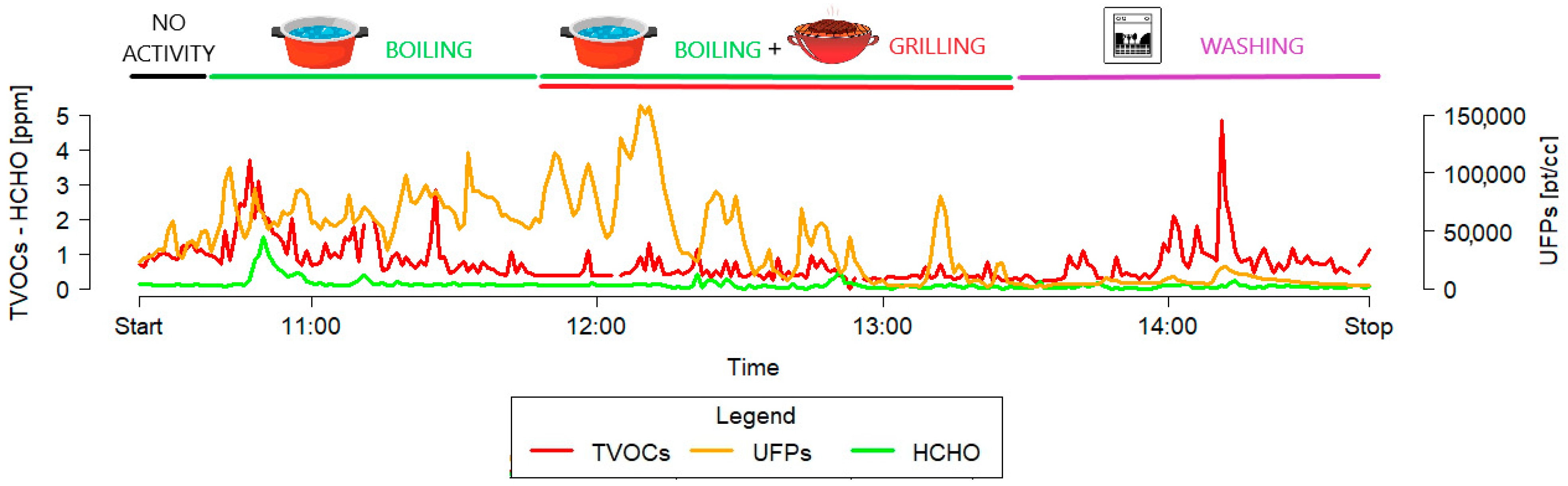
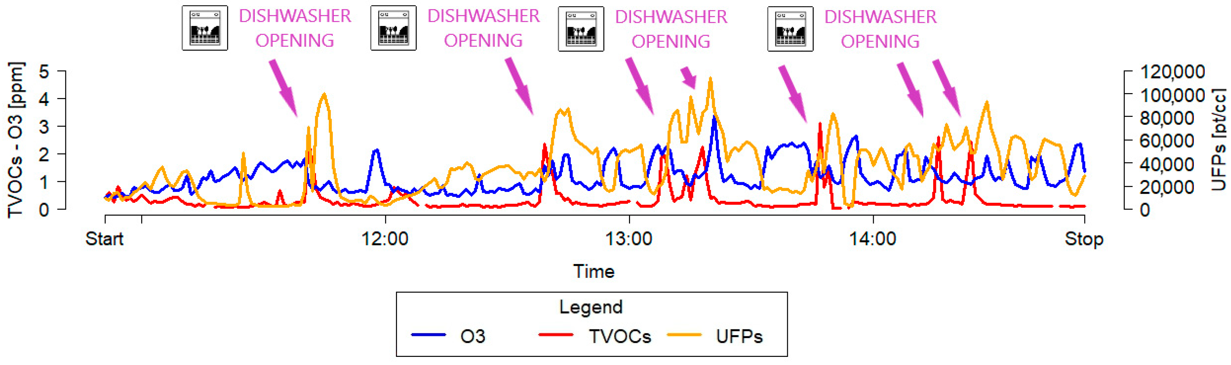
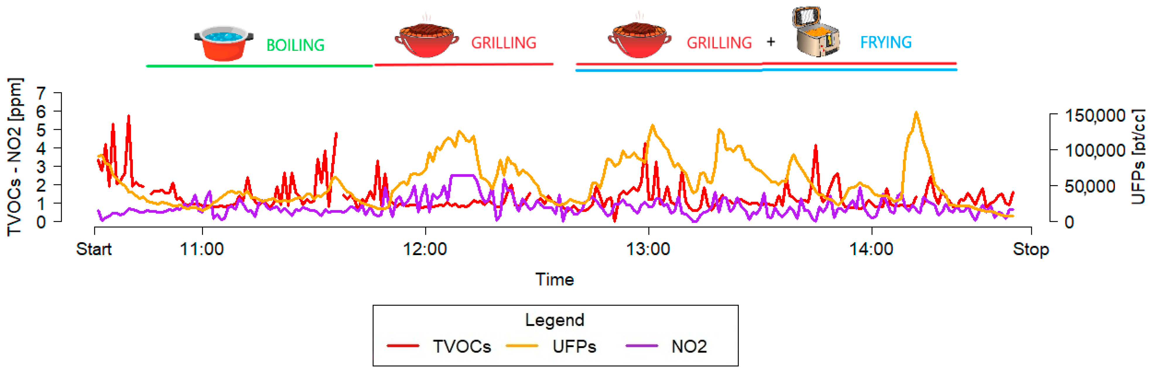
3.2. Short-Term and Real-Time Contamination Trends

The analysis of the video recordings allowed for a preliminary correlation of short-term concentration trends and peaks with specific events, such as the opening of the dishwasher or oven, and different cooking methods. This analysis allowed for the linking of activities to a group of specific pollutants and the identification of short-term trends and the respective sources. The following figures illustrate some examples of time–activity analysis (Figure 1, Figure 2, Figure 3 and Figure 4).

4. Discussion

4.1. Impact of Activities on IAQ

The preliminary analysis not only confirmed that cooking activities likely exert a statistically significant influence on the concentrations of the majority of selected pollutants (Figures S1 and S2) [29,30] but also revealed that cleaning activities have a measurable impact on the concentrations of certain pollutants, such as the TVOCs, HCHO and NO2 (Figures S3 and S4). The only pollutant inversely correlated with these activities was O3. The alteration of IAQ by direct emissions of air pollutants from cooking and washing activities is not unexpected, as it is well known that gas-based combustion processes cause the formation of NOx and the release of UFPs and that the emission of aldehydes and VOCs during cooking is primarily the result of thermal degradation of the food components [31,32]. For instance, cooking at high temperatures, especially frying and grilling, leads to the breakdown of fats and oils, resulting in the formation of aldehydes and VOCs [33,34]. Moreover, the combustion of natural gas in gas stoves can release combustion by-products, including HCHO [35]. It is worth noting that the specific types and amounts of aldehydes and VOCs emitted can vary depending on the cooking methods; ingredients and kitchen conditions (e.g., room volumes, ventilation, etc.) [36]. The opposite behavior of O3 (inversely correlated with cooking) can be interpreted as a result of ozonolysis reactions involving the reaction of O3 with unsaturated organic compounds, particularly alkenes or alkynes, emitted by the thermal breakdown or pyrolysis of organic compounds present in food. This could also be interpreted in light of the supposed absence of specific indoor sources originating direct emissions of O3 in restaurant kitchens.
Some other noteworthy aspects emerged from the study of short-term variations in the time–activity data. First, statistically significant differences among the types of activities were observed for the TVOCs, HCHO, NO2 and UFPs in the winter (Figures S5–S8) and for O3, the TVOCs and HCHO in the summer (Figures S5, S6 and S9). In the winter, NO2 exhibited statistically higher median concentrations during frying and grilling compared to boiling (+67% and +22%, respectively). Similarly, the median UFP concentrations were also statistically influenced by cooking activities, particularly frying (+53%) and boiling (+8%). These results are consistent with previous findings [37] and were more pronounced in the winter than in the summer. This discrepancy can be attributed to the fact that, in the winter, more time was spent cooking, particularly frying (24 min per restaurant in the winter vs. 13 min in the summer, on average). Additionally, the data indicated that surface cleaning significantly influenced the median NO2 concentrations compared to other activities (i.e., about +50% vs. washing activities and +42.5% vs. grilling). This result could be expected when comparing surface cleaning and washing activities, but it was quite challenging to interpret in the case of grilling activities. One hypothesis could be that the use of cleaning products, in the presence of light, leads to the generation of HONO, which is a typical interferent in the measurement of NO2 [38,39].
In terms of the TVOCs, a few seasonal differences were observed among the activities. Specifically, frying had a certain impact on the IAQ (+22% compared to boiling) in the winter, whereas, in the hot season, the highest median TVOC concentrations were recorded during boiling compared to the other types of cooking (i.e., >+40%). In the winter, the median HCHO concentrations were significantly lower during grilling (−50%) than during boiling and frying. In the summer, the highest HCHO median concentrations were again recorded during boiling but less markedly (+10% vs. grilling and +16% vs. frying).
Moreover, washing either by hand or using a dishwasher, had a greater impact on the TVOC and HCHO indoor concentrations than cooking both in the winter and summer (Figures S5 and S6). This outcome highlights the key impact of these activities on the emissions and resulting indoor air concentrations of these organic compounds. In a nutshell, cleaning products emerged as a significant source strongly impacting the IAQ in both seasons. The use of detergents results in the air emission of various VOCs, including terpenes such as d-limonene, α-pinene and p-cymene [1,40]. The release of these pollutants into the air, in the presence of O3, can induce ozonolysis reactions, resulting in the production of carbonyl compounds such as HCHO. Since the O3 concentrations are typically higher in the summer, this could explain the higher average HCHO concentrations measured during washing activities in the summer compared to the winter (+86%) (Table S1) [41].

4.2. Temporal Analysis

Thanks to the video analysis, it was possible to observe the high temporal resolution trends of the pollutant concentrations, correlating them with the professional activities (or events) simultaneously performed in the kitchen.
As illustrated in the examples reported in Figure 1, Figure 3 and Figure 4, the UFP and NO2 concentration peaks are primarily associated with cooking activities, particularly frying and grilling. This trend aligns with the findings reported above, with significantly higher concentrations of these pollutants during cooking, especially when high flames were used to reach high cooking temperatures, which can lead to the air emission of carbon- and oil- based nanoparticles in the indoor air during frying and grilling. This association between cooking and both UFP and NO2 concentrations is widely acknowledged in the literature, especially for grilling activities that generate large amounts of ultrafine and fine particles [42,43,44]. Moreover, TVOC and UFP concentration peaks were also observed (Figure 3 and Figure 4) during frying and grilling activities. Frying was also associated with short-term peaks of HCHO (Figure 4). As widely reported in the literature, frying is known as a high-emission cooking method, especially for some specific aldehydes (i.e., HCHO and acrolein) and UFPs as well [42,45].
The TVOC concentration peaks were also typically associated with washing activities (Figure 1). This finding is depicted in more detail in Figure 2, which reports the concentration trends of three key pollutants investigated in one of the restaurants during the summer campaign. The video analysis revealed that high and short-term TVOC peaks could be correlated to the opening of the dishwasher door, which can be attributed to the evaporation of VOCs from the hot washing water [46]. Interestingly, each TVOC peak (represented by the red line) was followed by a UFP peak and a slight reduction in the O3 concentration. This strict relationship between the TVOCs, UFPs and O3 could again be interpreted in light of the occurrence of ozonolysis reactions leading to the production of aldehydes (e.g., HCHO and acetaldehyde), oxidized VOCs and secondary organic aerosols in the ultrafine size fraction [47].

4.3. Strengths and Weaknesses

The study has several strengths that contribute to the understanding of pollutant emissions in restaurant kitchens. The quantification of the impact of various kitchen activities on pollutant emissions, including dishwashing and surface cleaning, addresses a significant gap in the existing literature. Another notable strength was the use of a real-time and multipollutant monitoring approach coupled with cameras, which allowed us to collect comprehensive, detailed and minute-by-minute information, enabling a thorough characterization of the pollutant concentration levels and their connection with short-term pollution sources. However, the study also has some limitations that should be acknowledged. The investigation was conducted in a limited number of restaurants, which might result in findings that are specific to those indoor spaces rather than providing a representative overview of the restaurant kitchens in Italy. Additionally, the large variability in occupational activities performed day by day and across kitchens introduces a certain degree of unpredictability, making it challenging to derive generalized conclusions and requiring a case-by-case explanation for the observed concentration levels. Another limitation of the study is the reliance on real-time data from alternative monitoring methods rather than reference-grade instruments. These methods, particularly those used for measuring HCHO, O3 and NO2, are typically characterized by lower precision and accuracy. While we were able to correct the formaldehyde levels using reliable monitoring methods, we were unable to do the same for O3 and NO2. Despite these limitations, this study can contribute to providing useful insights into the understanding of pollutant dynamics in restaurant kitchens, emphasizing the need for further data analysis and research to achieve a broader generalizability.

5. Conclusions

This study aimed to evaluate the impact of the main activities carried out within restaurant kitchens.
The following conclusions emerged from this work:
-
Cooking and also washing and cleaning activities played a key role in affecting the IAQ in professional kitchens.
-
Cooking activities had a significantly impact on the IAQ, especially in the winter, mainly for UFPs, NO2, the TVOCs and HCHO. In particular, UFPs in the kitchens were notably high in the winter (median level of 32.500 and higher than 80.000 pt/cm3 while frying), nearly tripled with respect to the summer (11.700 pt/cm3) (Table S1 and Figure S8).
-
Washing activities exerted a statistically significant impact on the TVOC and HCHO indoor concentrations in both seasons. The relevance of washing and cleaning became more evident in the winter, when windows were closed, leading to a 50–61% increase in the TVOC concentrations and a 50–75% increase in HCHO concentrations during kitchen surface cleaning compared to cooking (Table 2 and Table 4).
-
Specific events, such as the opening of the dishwasher, were strongly correlated with short-term peaks of TVOCs and UFPs (Figure 2).
-
A time-dependent relationship between O3 and UFPs, TVOCs and sometimes also HCHO was observed in some restaurants, probably due to the occurrence of ozonolysis reactions (Figure 2).
Possible developments of this study may involve a more detailed and systematic analysis of the concentration peaks, as already done in [48], and the application of multivariate analysis techniques to gain a deeper understanding of these complex data and how they relate to real-world scenarios. Moreover, machine learning approaches could be used to improve the data quality of low-cost sensor devices [49].

Supplementary Materials

The following supporting information can be downloaded at https://www.mdpi.com/article/10.3390/atmos15080976/s1: Figure S1. Violin plots of indoor pollutant concentrations measured in the winter during or in the absence of cooking activities. *: pMW < 0.01 and **: pMW < 0.001; Figure S2. Violin plots of indoor pollutant concentrations measured in the winter during or in the absence of cooking activities. *: pMW < 0.01 and **: pMW < 0.001; Figure S3. Violin plots of indoor pollutant concentrations measured in the summer during or in the absence of washing activities. *: pMW < 0.01 and **: pMW < 0.001; Figure S4. Violin plots of indoor pollutant concentrations measured in the summer during or in the absence of washing activities. *: pMW < 0.01 and **: pMW < 0.001; Figure S5. Box plots of the TVOC levels for the main activities observed during the monitoring campaigns (winter and summer, respectively); Figure S6. Box plots of the HCHO levels for the main activities identified during the monitoring campaigns (winter and summer, respectively); Figure S7. Box plots of the NO2 levels for the main activities identified during the identified during the monitoring campaigns (winter and summer, respectively); Figure S8. Box plots of the UFP levels for the main activities identified during the identified during the monitoring campaigns (winter and summer, respectively); Figure S9. Box plots of the O3 levels for the main activities identified during the identified during the monitoring campaigns (winter and summer, respectively); Table S1. Indoor concentrations of the air pollutants and physical parameters (temperature and relative humidity) monitored on a real-time basis in restaurant kitchens.

Author Contributions

Conceptualization, M.K. and A.C. (Andrea Cattaneo); methodology, A.C. (Andrea Cattaneo), M.K. and C.D.; formal analysis, M.K. and D.C.; investigation, M.K.; resources, D.M.C., C.D., A.C. (Andrea Cattaneo) and A.S.; data curation, M.K. and D.C.; writing—original draft preparation, M.K., D.C. and A.C. (Andrea Cattaneo); writing—review and editing, M.K., D.C., F.B., A.C. (Alessio Carminati), G.F., S.R., C.Z., R.L.D.V., G.D.V., A.S., V.G.M., C.D., M.C., A.C. (Andrea Cattaneo) and D.M.C.; supervision, A.C. (Andrea Cattaneo), C.D., V.G.M., A.S. and D.M.C. All authors have read and agreed to the published version of the manuscript.

Funding

This research was supported by internal funding (RAHH research group and Doctoral School, University of Insubria).

Institutional Review Board Statement

Not applicable.

Informed Consent Statement

Not applicable.

Data Availability Statement

The original contributions presented in the study are included in the article/supplementary material, further inquiries can be directed to the corresponding authors.

Acknowledgments

R. Perna and G. Carugati are kindly acknowledged for their help in the chemical analysis.

Conflicts of Interest

The authors declare no conflicts of interest.

References

  1. Huang, Y.; Ho, S.S.H.; Ho, K.F.; Lee, S.C.; Yu, J.Z.; Louie, P.K.K. Characteristics and Health Impacts of VOCs and Carbonyls Associated with Residential Cooking Activities in Hong Kong. J. Haz. Mater. 2011, 186, 344–351. [Google Scholar] [CrossRef] [PubMed]
  2. Lee, Y.-Y.; Park, H.; Seo, Y.; Yun, J.; Kwon, J.; Park, K.-W.; Han, S.-B.; Oh, K.C.; Jeon, J.-M.; Cho, K.-S. Emission Characteristics of Particulate Matter, Odors, and Volatile Organic Compounds from the Grilling of Pork. Environ. Res. 2020, 183, 109162. [Google Scholar] [CrossRef]
  3. Peng, C.-Y.; Lan, C.-H.; Lin, P.-C.; Kuo, Y.-C. Effects of Cooking Method, Cooking Oil, and Food Type on Aldehyde Emissions in Cooking Oil Fumes. J. Haz. Mater. 2017, 324, 160–167. [Google Scholar] [CrossRef]
  4. Chiang, T.-A.; Wu, P.-F.; Ko, Y.-C. Identification of Carcinogens in Cooking Oil Fumes. Environ. Res. 1999, 81, 18–22. [Google Scholar] [CrossRef]
  5. Chen, C.-Y.; Kuo, Y.-C.; Wang, S.-M.; Wu, K.-R.; Chen, Y.-C.; Tsai, P.-J. Techniques for Predicting Exposures to Polycyclic Aromatic Hydrocarbons (PAHs) Emitted from Cooking Processes for Cooking Workers. Aerosol Air Qual. Res. 2019, 19, 307–317. [Google Scholar] [CrossRef]
  6. Seaman, V.Y.; Bennett, D.H.; Cahill, T.M. Indoor Acrolein Emission and Decay Rates Resulting from Domestic Cooking Events. Atmos. Environ. 2009, 43, 6199–6204. [Google Scholar] [CrossRef]
  7. Wolkoff, P.; Nielsen, G.D. Non-Cancer Effects of Formaldehyde and Relevance for Setting an Indoor Air Guideline. Environ. Int. 2010, 36, 788–799. [Google Scholar] [CrossRef]
  8. Meininghaus, R. Risk Assessment of Sensory Irritants in Indoor Air—A Case Study in a French School. Environ. Int. 2003, 28, 553–557. [Google Scholar] [CrossRef] [PubMed]
  9. Rovelli, S.; Cattaneo, A.; Fazio, A.; Spinazzè, A.; Borghi, F.; Campagnolo, D.; Dossi, C.; Cavallo, D.M. VOCs Measurements in Residential Buildings: Quantification via Thermal Desorption and Assessment of Indoor Concentrations in a Case-Study. Atmosphere 2019, 10, 57. [Google Scholar] [CrossRef]
  10. Campagnolo, D.; Saraga, D.E.; Cattaneo, A.; Spinazzè, A.; Mandin, C.; Mabilia, R.; Perreca, E.; Sakellaris, I.; Canha, N.; Mihucz, V.G.; et al. VOCs and Aldehydes Source Identification in European Office Buildings—The OFFICAIR Study. Build. Environ. 2017, 115, 18–24. [Google Scholar] [CrossRef]
  11. Kumar, P.; Martani, C.; Morawska, L.; Norford, L.; Choudhary, R.; Bell, M.; Leach, M. Indoor Air Quality and Energy Management through Real-Time Sensing in Commercial Buildings. Energy Build. 2016, 111, 145–153. [Google Scholar] [CrossRef]
  12. Ródenas García, M.; Spinazzé, A.; Branco, P.T.B.S.; Borghi, F.; Villena, G.; Cattaneo, A.; Di Gilio, A.; Mihucz, V.G.; Gómez Álvarez, E.; Lopes, S.I.; et al. Review of Low-Cost Sensors for Indoor Air Quality: Features and Applications. Appl. Spectrosc. Rev. 2022, 57, 747–779. [Google Scholar] [CrossRef]
  13. Alves, C.A.; Vicente, E.D.; Evtyugina, M.; Vicente, A.M.P.; Sainnokhoi, T.-A.; Kováts, N. Cooking Activities in a Domestic Kitchen: Chemical and Toxicological Profiling of Emissions. Sci. Total Environ. 2021, 772, 145412. [Google Scholar] [CrossRef] [PubMed]
  14. Zhang, W.; Bai, Z.; Shi, L.; Son, J.H.; Li, L.; Wang, L.; Chen, J. Investigating Aldehyde and Ketone Compounds Produced from Indoor Cooking Emissions and Assessing Their Health Risk to Human Beings. J. Environ. Sci. 2023, 127, 389–398. [Google Scholar] [CrossRef] [PubMed]
  15. Andersen, P.C.; Williford, C.J.; Birks, J.W. Miniature Personal Ozone Monitor Based on UV Absorbance. Anal. Chem. 2010, 82, 7924–7928. [Google Scholar] [CrossRef]
  16. Black, D.R.; Harley, R.A.; Hering, S.V.; Stolzenburg, M.R. A New, Portable, Real-Time Ozone Monitor. Environ. Sci. Technol. 2000, 34, 3031–3040. [Google Scholar] [CrossRef]
  17. Deville Cavellin, L.; Weichenthal, S.; Tack, R.; Ragettli, M.S.; Smargiassi, A.; Hatzopoulou, M. Investigating the Use Of Portable Air Pollution Sensors to Capture the Spatial Variability Of Traffic-Related Air Pollution. Environ. Sci. Technol. 2016, 50, 313–320. [Google Scholar] [CrossRef]
  18. Lin, C.; Gillespie, J.; Schuder, M.D.; Duberstein, W.; Beverland, I.J.; Heal, M.R. Evaluation and Calibration of Aeroqual Series 500 Portable Gas Sensors for Accurate Measurement of Ambient Ozone and Nitrogen Dioxide. Atmos. Environ. 2015, 100, 111–116. [Google Scholar] [CrossRef]
  19. McGill, G.; Oyedele, L.O.; McAllister, K. Case Study Investigation of Indoor Air Quality in Mechanically Ventilated and Naturally Ventilated UK Social Housing. Int. J. Sust. Built Environ. 2015, 4, 58–77. [Google Scholar] [CrossRef]
  20. Zhu, Y.; Yu, N.; Kuhn, T.; Hinds, W.C. Field Comparison of P-Trak and Condensation Particle Counters. Aerosol Sci. Technol. 2006, 40, 422–430. [Google Scholar] [CrossRef]
  21. Duvall, R.; Long, R.; Beaver, M.; Kronmiller, K.; Wheeler, M.; Szykman, J. Performance Evaluation and Community Application of Low-Cost Sensors for Ozone and Nitrogen Dioxide. Sensors 2016, 16, 1698. [Google Scholar] [CrossRef]
  22. Spinelle, L.; Gerboles, M.; Aleixandre, M. Performance Evaluation of Amperometric Sensors for the Monitoring of O3 and NO2 in Ambient Air at Ppb Level. Procedia Eng. 2015, 120, 480–483. [Google Scholar] [CrossRef]
  23. Huang, K.; Song, J.; Feng, G.; Chang, Q.; Jiang, B.; Wang, J.; Sun, W.; Li, H.; Wang, J.; Fang, X. Indoor Air Quality Analysis of Residential Buildings in Northeast China Based on Field Measurements and Longtime Monitoring. Build. Environ. 2018, 144, 171–183. [Google Scholar] [CrossRef]
  24. Gilden, R.C.; Friedmann, E.J.; Spanier, A.J.; Hennigan, C.J. Indoor Air Quality Monitoring in Baltimore City, MD Head Start Centers. Int. J. Environ. Sci. Technol. 2022, 19, 11523–11530. [Google Scholar] [CrossRef]
  25. Flueckiger, J.; Ko, F.K.; Cheung, K.C. Microfabricated Formaldehyde Gas Sensors. Sensors 2009, 9, 9196–9215. [Google Scholar] [CrossRef]
  26. Boniardi, L.; Borghi, F.; Straccini, S.; Fanti, G.; Campagnolo, D.; Campo, L.; Olgiati, L.; Lioi, S.; Cattaneo, A.; Spinazzè, A.; et al. Commuting by Car, Public Transport, and Bike: Exposure Assessment and Estimation of the Inhaled Dose of Multiple Airborne Pollutants. Atmos. Environ. 2021, 262, 118613. [Google Scholar] [CrossRef]
  27. Feltovich, N. Nonparametric Tests of Differences in Medians: Comparison of the Wilcoxon–Mann–Whitney and Robust Rank-Order Tests. Exp. Econ. 2003, 6, 273–297. [Google Scholar] [CrossRef]
  28. Emerson, R.W. Bonferroni Correction and Type I Error. J. Vis. Impair. Blind. 2020, 114, 77–78. [Google Scholar] [CrossRef]
  29. Amouei Torkmahalleh, M.; Gorjinezhad, S.; Unluevcek, H.S.; Hopke, P.K. Review of Factors Impacting Emission/Concentration of Cooking Generated Particulate Matter. Sci. Total Environ. 2017, 586, 1046–1056. [Google Scholar] [CrossRef]
  30. Wang, L.; Xiang, Z.; Stevanovic, S.; Ristovski, Z.; Salimi, F.; Gao, J.; Wang, H.; Li, L. Role of Chinese Cooking Emissions on Ambient Air Quality and Human Health. Sci. Total Environ. 2017, 589, 173–181. [Google Scholar] [CrossRef]
  31. See, S.W.; Balasubramanian, R. Chemical Characteristics of Fine Particles Emitted from Different Gas Cooking Methods. Atmos. Environ. 2008, 42, 8852–8862. [Google Scholar] [CrossRef]
  32. Atamaleki, A.; Motesaddi Zarandi, S.; Massoudinejad, M.; Hesam, G.; Naimi, N.; Esrafili, A.; Fakhri, Y.; Mousavi Khaneghah, A. Emission of Aldehydes from Different Cooking Processes: A Review Study. Air Qual. Atmos. Health 2022, 15, 1183–1204. [Google Scholar] [CrossRef]
  33. Bassam, S.M.; Noleto-Dias, C.; Farag, M.A. Dissecting Grilled Red and White Meat Flavor: Its Characteristics, Production Mechanisms, Influencing Factors and Chemical Hazards. Food Chem. 2022, 371, 131139. [Google Scholar] [CrossRef]
  34. Takhar, M.; Li, Y.; Ditto, J.C.; Chan, A.W.H. Formation Pathways of Aldehydes from Heated Cooking Oils. Environ. Sci. Process. Impacts 2023, 25, 165–175. [Google Scholar] [CrossRef] [PubMed]
  35. Poppendieck, D.; Gong, M. Simmering Sauces! Elevated Formaldehyde Concentrations from Gas Stove Burners; Indoor Air: Philadelphia, PA, USA, 2018. [Google Scholar]
  36. Kim, S.; Hong, S.-H.; Bong, C.-K.; Cho, M.-H. Characterization of Air Freshener Emission: The Potential Health Effects. J. Toxicol. Sci. 2015, 40, 535–550. [Google Scholar] [CrossRef]
  37. Dennekamp, M.; Howarth, S.; Dick, C.A.J.; Cherrie, J.W.; Donaldson, K.; Seaton, A. Ultrafine Particles and Nitrogen Oxides Generated by Gas and Electric Cooking. Occup. Environ. Med. 2001, 58, 511–516. [Google Scholar] [CrossRef] [PubMed]
  38. Spinelle, L.; Gerboles, M.; Kok, G.; Persijn, S.; Sauerwald, T. Review of Portable and Low-Cost Sensors for the Ambient Air Monitoring of Benzene and Other Volatile Organic Compounds. Sensors 2017, 17, 1520. [Google Scholar] [CrossRef]
  39. Gómez Alvarez, E.; Sörgel, M.; Gligorovski, S.; Bassil, S.; Bartolomei, V.; Coulomb, B.; Zetzsch, C.; Wortham, H. Light-Induced Nitrous Acid (HONO) Production from NO2 Heterogeneous Reactions on Household Chemicals. Atmos. Environ. 2014, 95, 391–399. [Google Scholar] [CrossRef]
  40. Xu, C.; Chen, J.; Zhang, X.; Cai, K.; Chen, C.; Xu, B. Emission Characteristics and Quantitative Assessment of the Health Risks of Cooking Fumes during Outdoor Barbecuing. Environ. Pollut. 2023, 323, 121319. [Google Scholar] [CrossRef]
  41. Ling, Z.H.; Zhao, J.; Fan, S.J.; Wang, X.M. Sources of Formaldehyde and Their Contributions to Photochemical O3 Formation at an Urban Site in the Pearl River Delta, Southern China. Chemosphere 2017, 168, 1293–1301. [Google Scholar] [CrossRef]
  42. Xiang, J.; Hao, J.; Austin, E.; Shirai, J.; Seto, E. Characterization of Cooking-Related Ultrafine Particles in a US Residence and Impacts of Various Intervention Strategies. Sci. Total Environ. 2021, 798, 149236. [Google Scholar] [CrossRef]
  43. Buonanno, G.; Stabile, L.; Morawska, L.; Russi, A. Children Exposure Assessment to Ultrafine Particles and Black Carbon: The Role of Transport and Cooking Activities. Atmos. Environ. 2013, 79, 53–58. [Google Scholar] [CrossRef]
  44. Wong, T.W. Household Gas Cooking: A Risk Factor for Respiratory Illnesses in Preschool Children. Arch. Dis. Child. 2004, 89, 631–636. [Google Scholar] [CrossRef]
  45. Li, Y.; Ou, J.; Huang, C.; Liu, F.; Ou, S.; Zheng, J. Chemistry of Formation and Elimination of Formaldehyde in Foods. Trends Food Sci. Technol. 2023, 139, 104134. [Google Scholar] [CrossRef]
  46. Dinh, T.-V.; Kim, S.-Y.; Son, Y.-S.; Choi, I.-Y.; Park, S.-R.; Sunwoo, Y.; Kim, J.-C. Emission Characteristics of VOCs Emitted from Consumer and Commercial Products and Their Ozone Formation Potential. Environ. Sci. Pollut. Res. 2015, 22, 9345–9355. [Google Scholar] [CrossRef] [PubMed]
  47. Fan, Z.; Weschler, C.J.; Han, I.-K.; Zhang, J. (Jim) Co-Formation of Hydroperoxides and Ultra-Fine Particles during the Reactions of Ozone with a Complex VOC Mixture under Simulated Indoor Conditions. Atmos. Environ. 2005, 39, 5171–5182. [Google Scholar] [CrossRef]
  48. Dons, E.; Laeremans, M.; Orjuela, J.P.; Avila-Palencia, I.; de Nazelle, A.; Nieuwenhuijsen, M.; Van Poppel, M.; Carrasco-Turigas, G.; Standaert, A.; De Boever, P.; et al. Transport most likely to cause air pollution peak exposures in everyday life: Evidence from over 2000 days of personal monitoring. Atmos. Environ. 2019, 213, 424–432. [Google Scholar] [CrossRef]
  49. Chojer, H.; Branco, P.T.B.S.; Martins, F.G.; Alvim-Ferraz, M.C.M.; Sousa, S.I.V. Can data reliability of low-cost sensor devices for indoor air particulate matter monitoring be improved? —An approach using machine learning. Atmos. Environ. 2022, 286, 119251. [Google Scholar] [CrossRef]
Figure 1. Example of time trends of the TVOCs, HCHO and UFPs vs. kitchen activities performed in one of the investigated restaurants.
Atmosphere 15 00976 g001
Figure 2. Example of time trends of the TVOCs, O3 and UFPs in a restaurant. The purple arrows represent the exact moments when the dishwasher door was opened.
Atmosphere 15 00976 g002
Figure 3. Example of time trends of the TVOCs, NO2 and UFPs vs. kitchen activities in a restaurant.
Atmosphere 15 00976 g003
Figure 4. Example of time trends of the TVOCs, HCHO and UFPs vs. kitchen activities performed in one of the investigated restaurants.
Atmosphere 15 00976 g004
Table 1. The main characteristics of the real-time instrumentation used to assess the air quality in the kitchens.
PollutantInstrumentBrandTechnologyRangeLimit of Detection (LOD)Literature Reference
Ozone (O3)POM
(Personal Ozone Monitor)
2B TechnologiesUV absorbance0 ppb–10 ppm0.003 ppm[15,16]
TVOCs *Aeroqual monitor
Series 500
Aeroqual
Auckland
New Zealand
Photoionization detector (PID)0–20 ppm0.01 ppm[17,18]
Formaldehyde (HCHO)HAL-HFX205Hal Technology, Fontana, CA, USAElectrochemical sensing technology0–10 ppmv0.01 ppmv[19]
Ultrafine particles (UFPs)P-Trak 8525TSI Incorporated, Shoreview, MN, USACondensation Particle Counter (CPC)0–105
particles/cm3
0.02–1 µm **[20]
Nitrogen dioxide (NO2)CairClip monitorCairpol; La Roche Blanche, FranceElectrochemical sensor0–250 ppb1.692 μg/m3[21,22]
Carbon dioxide (CO2) ***Telaire 7001GE sensing, Goleta, CA, USANon-dispersive infrared (NDIR) sensor0–10,000 ppm1 ppm[23]
Temperature (T) and Relative Humidity (RH)Hobo U12Onset Computer Corporation, Bourne, MA, USAInternal sensors−20 °C to
+70 °C
5–95%
N.A.
* Total Volatile Organic Compounds. ** Size range of detectable particles. *** To data recording, the Telaire sensor was connected to the Hobo U12 datalogger.
Table 2. M–W test results and median percentage differences among the groups for the TVOC levels measured during the winter campaign. The p-value refers to M–W tests. Row vs. column matrix.
TVOCs in WinterBoilingGrillingFryingHandwashingDishwasher Running
grilling−26%
(p < 0.001)
frying(p = 0.7)+22% (p < 0.001)
handwashing+6%
(p < 0.05)
+26% (p < 0.001)(p = 0.1)
dishwasher running+6%
(p < 0.05)
+26% (p < 0.001)(p = 0.4)(p = 0.4)
surface cleaning+50% (p < 0.001)+61% (p < 0.001)+50% (p < 0.001)+47% (p < 0.001)+47% (p < 0.001)
Table 3. M–W test results and median percentage differences among the groups for the TVOC levels measured during the summer campaign. The p-value refers to M–W tests. Row vs. column matrix.
TVOCs in Summer Boiling Grilling Frying Handwashing Dishwasher Running
grilling−41%
(p < 0.001)
frying−46%
(p < 0.001)
(p = 0.9)
handwashing−13%
(p < 0.001)
+49% (p < 0.001)+51% (p < 0.001)
dishwasher running−18%
(p < 0.01)
+28% (p < 0.001)+31% (p < 0.001)−29%
(p < 0.001)
surface cleaning−41%
(p < 0.05)
(p = 0.9)(p = 0.9)−49%
(p < 0.01)
(p = 0.1)
Table 4. Median relative differences among the groups for the HCHO levels measured during the winter campaign. The p-value refers to M–W tests. Row vs. column matrix.
HCHO in Winter Boiling Grilling Frying Handwashing Dishwasher Running
grilling−50%
(p < 0.001)
frying(p = 0.8)+50%
(p < 0.01)
handwashing+33% (p < 0.001)+67% (p < 0.001)+33% (p < 0.001)
dishwasher running+33% (p < 0.001)+67% (p < 0.001)+33%
(p < 0.01)
+16% (p < 0.001)
surface cleaning+47%
(p < 0.01)
+75% (p < 0.001)+50% (p < 0.001)(p = 0.9)(p = 0.2)
Table 5. Median relative differences among the groups for the HCHO levels measured during the summer campaign. The p-value refers to M–W tests. Row vs column matrix.
HCHO in Summer Boiling Grilling Frying Handwashing Dishwasher Running
grilling−10%
(p < 0.001)
frying−16%
(p < 0.01)
(p = 0.5)
handwashing(p = 0.1)+62%
(p < 0.001)
+64%
(p < 0.001)
dishwasher running(p = 0.2)(p = 0.06)+42%
(p < 0.05)
−38%
(p < 0.01)
surface cleaning−22%
(p < 0.001)
−18%
(p < 0.01)
(p = 0.07)−49%
(p < 0.001)
−38%
(p < 0.001)
Table 6. Median relative differences among the groups for the NO2 levels measured during the winter campaign. The p-value refers to M–W tests. Row vs. column matrix.
NO2 in
Winter
Boiling Grilling Frying Handwashing Dishwasher Running
grilling+22%
(p < 0.001)
frying+67%
(p < 0.001)
+57%
(p < 0.001)
handwashing(p = 0.4)−22%
(p < 0.001)
−67%
(p < 0.001)
dishwasher running(p = 0.6)−17%
(p < 0.001)
−65%
(p < 0.01)
(p = 0.6)
surface cleaning(p = 0.07)+42.5% (p < 0.001)−26%
(p < 0.05)
+55%
(p < 0.05)
+52.5% (p < 0.05)
Table 7. Median relative differences among the groups for the UFP levels measured during the winter campaign. The p-value refers to M–W tests. Row vs. column matrix.
UFP in Winter Boiling Grilling Frying Handwashing Dishwasher Running
grilling−8%
(p < 0.05)
frying+53%
(p < 0.001)
+57%
(p < 0.001)
handwashing−10%
(p < 0.05)
(p = 0.9)−58%
(p < 0.001)
dishwasher running−8%
(p < 0.01)
(p = 0.9)−57%
(p < 0.001)
(p = 0.9)
surface cleaning−47%
(p < 0.001)
−42%
(p < 0.05)
−54%
(p < 0.001)
−41%
(p < 0.01)
−42%
(p < 0.01)
Table 8. Median relative differences among the groups for the O3 levels measured during the summer campaign. The p-value refers to M–W tests. Row vs. column matrix.
O3 in Summer Boiling Grilling Frying Handwashing Dishwasher Running
grilling+17% (p < 0.05)
frying−35% (p < 0.001)−45%
(p < 0.001)
handwashing−12% (p < 0.001)−25%
(p < 0.001)
+35% (p < 0.05)
dishwasher running(p = 0.5)(p = 0.1)+35% (p < 0.001)+12% (p < 0.001)
surface cleaning+10.5% (p < 0.05)(p = 0.7)+42% (p < 0.01)+21%
(p < 0.01)
(p = 0.1)
Disclaimer/Publisher’s Note: The statements, opinions and data contained in all publications are solely those of the individual author(s) and contributor(s) and not of MDPI and/or the editor(s). MDPI and/or the editor(s) disclaim responsibility for any injury to people or property resulting from any ideas, methods, instructions or products referred to in the content.

