Article

Evaluation of Near-Taiwan Strait Sea Surface Wind Forecast Based on PanGu Weather Prediction Model

1
Key Laboratory of Marine Hazards Forecasting, National Marine Environment Forecasting Center, Beijing 100081, China
2
National Meteorological Center, Beijing 100081, China
3
Institute of Science and Technology, China Three Gorges Corporation, Beijing 101100, China
*
Author to whom correspondence should be addressed.
Atmosphere 2024, 15(8), 977; https://doi.org/10.3390/atmos15080977
Submission received: 21 June 2024 / Revised: 10 August 2024 / Accepted: 12 August 2024 / Published: 15 August 2024
(This article belongs to the Section Meteorology)

Abstract

:
Utilizing observed wind speed and direction data from observation stations near the Taiwan Strait and ocean buoys, along with forecast data from the EC model, GRAPES_GFS model, and PanGu weather prediction model within the same period, RMSE, MAE, CC, and other parameters were calculated. To comparatively evaluate the forecasting performance of the PanGu weather prediction model on the sea surface wind field near the Taiwan Strait from 00:00 on 1 June 2023, to 23:00 on 31 May 2024. The PanGu weather prediction model is further divided into the ERA5 (PanGu) model driven by ERA5 initial fields and the GRAPES_GFS (PanGu) model driven by GRAPES_GFS initial fields. The main conclusions are as follows: (1) over a one-year evaluation period, for wind speed forecasts with lead times of 0 h to 120 h in the Taiwan Strait region, the overall forecasting skill of the PanGu weather prediction model is superior to that of the model forecasts; (2) different initial fields input into the PanGu weather prediction model lead to different final forecast results, with better initial field data corresponding to forecast results closer to observations, thus indicating the operational transferability of the PanGu model in smaller regions; (3) regarding forecasts of wind speed categories, the credibility of the results is high when the wind speed level is ≤7, and the PanGu weather prediction model performs better among similar forecasts; (4) although the EC model’s wind direction forecasts are closer to the observation field results, the PanGu weather forecasting model also provides relatively accurate and rapid forecasts of the main wind directions within a shorter time frame.

1. Introduction

The sea surface wind field is one of the most fundamental and crucial elements in physical oceanography and marine meteorology. Oceanic meteorological disasters such as strong winds, storm surges, and waves are directly or indirectly related to it [1], influencing the coupled processes of the atmosphere and ocean [2]. Moreover, it plays an important role in studying and understanding global water circulation, energy circulation, carbon dioxide circulation, climate change [3], wind energy generation [4,5,6], maritime military decision-making [7,8], disaster prevention, and mitigation [9].
Currently, the mainstream method of nearshore wind field forecast is still numerical weather prediction (NWP). Major numerical weather forecast centers and developed countries worldwide have their global medium-range forecast models [7]. The foreign operational forecasting models mainly include the European Centre for Medium-Range Weather Forecasts (ECMWF), the Japan Meteorological Agency Global Spectral Model (JMA-GSM), the Geophysical Fluid Dynamics Laboratory (GFDL) Limited Area Numerical Forecast Model, the Naval Operational Global Atmospheric Prediction System (NO2GAPS), and the United Kingdom Meteorological Office Global Spectral Model (UK2MET), among others [10,11]. However, the development of NWP has been hampered by the fact that high-resolution numerical forecast systems often require significant computational resources and storage resources [12]. For example, using the WRF model, forecasting for the coastal waters of China at a resolution of 3 km requires over a thousand computational cores to continuously compute for over one hour to meet the forecast lead time requirements. Therefore, seeking a lighter and more efficient sea surface wind field forecasting model has become a research focus in recent years.
In recent years, with the rise in machine learning (ML), researchers have proposed applying deep learning (DL) research methods to the field of geophysics [13,14]. Thus, there have been initial attempts at DL models for wind field forecasting [15], hoping to overcome the shortcomings of NWP. Currently, most intelligent wind forecasting is single-point forecasting, such as for stations, wind turbines, etc. Usually one-dimensional time feature learning models are used, such as DNN [16], RNN [17], LSTM [18,19,20], etc. There is still limited research on DL models for two-dimensional field forecasting of sea surface wind fields. However, as we come to 2022, and intelligent forecasting large models applicable to meteorological forecasting have gradually emerged, these undoubtedly represent a breakthrough for solving the prediction of two-dimensional sea surface wind fields. DeepMind and Google have developed GraphCast [21], which can predict multiple meteorological elements at a spatial resolution of 0.25° × 0.25° for the next ten days within one minute, showing superior performance compared to previous ML-based weather forecasting models; Nvidia developed the FourCastNet [22] model, which can generate simple weather forecasts for one week in less than 2 s and has strong capabilities in precipitation and typhoon forecasting. Domestically, there have also been meteorological large models such as NowcastNet [23], SwinVRNN [24], the “Fuxi” meteorological large model [25], the “Fengwu” [26], etc. Among them, the most prominent forecasting capability is the PanGu-Weather [27] model from Huawei Cloud, which has surpassed the IFS forecast products of the European Centre for Medium-Range Weather Forecasts in some surface and atmospheric elements. It signifies the first instance where AI-based forecasting models have surpassed traditional numerical methods in both accuracy and speed. Compared with the traditional intelligent forecasting large models, the PanGu model has two main advantages: (i) The PanGu model’s network structure is a 3D Earth-specific transformer capable of adapting to the Earth’s coordinate system. During training, it inputs meteorological variables from 13 layers of five upper-air and four surface variables into a deep network. This architecture enables heterogeneous 3D meteorological data to be handled effectively, which is a capability lacking in traditional intelligent forecasting large models built on 2D neural networks. (ii) The PanGu model consists of four basic deep network models with forecast lead times of 1 h, 3 h, 6 h, and 24 h. For instance, when forecasting for 56 h, the model runs the 24-hour model twice, the 6-hour model once, and the 1-hour model twice. This approach, known as the “hierarchical temporal aggregation strategy”, reduces forecast iteration cycles, thereby minimizing iteration errors. Compared to previous approaches like the fixed 6-hour forecast model (FourCastNet), the PanGu model reduces iteration cycles, resulting in faster and more accurate forecasts.
However, the operational forecasts of sea surface wind fields are more concerned with small-scale regions. The performance of the PanGu model in small-scale regional forecasting remains uncertain. Hence, this article specifically focuses on the Taiwan Strait region which has significant strait effects [28] and obvious seasonal characteristics [29,30] to assess the predictive capability of the PanGu model for sea surface wind fields within a small regional area. Due to the limited update frequency of ERA5 data, these data are impractical for operational forecasting, so we also evaluate the PanGu model’s applicability in operational forecasting. Based on the two evaluation angles mentioned above, in this paper, observed buoy wind field data are used in the Taiwan Strait region in the summer of 2023 to comparatively evaluate the 10 m wind speed and wind direction products of the EC model [31], GRAPES_GFS model [32], and two groups of PanGu weather forecast models with different initial fields. The relative forecasting performance of the PanGu weather model to numerical weather forecast models for sea surface wind fields will be discussed. The impact of different initial fields on the forecast results of the PanGu forecast model will also be compared and analyzed, aiming to provide a reference for the application of intelligent forecasting large models in local small-area sea surface wind field forecasting. In Section 2, the data, experiments, and evaluation methods are introduced. The results of the experiment, including the wind speed, wind scale, and direction are presented in Section 3. Section 4 presents a conclusion and discussion.

2. Data, Experiments, and Methods

2.1. Data and Experiments

The data used in this study included buoy observation data in the Taiwan Strait region (as shown in Figure 1), EC [31] high-resolution grid 10 m wind field forecast data, GRAPES_GFS [32] 10 m wind field forecast data, and two groups of PanGu model’s 5-day 10 m wind field forecast data made with ERA5 re-analysis data and GRAPES_GFS analysis data as initial fields.
The two groups of PanGu weather forecast models are as follows:
  • ERA5 (PanGu): Pre-test with ERA5 reanalysis data as the initial field. This experiment represents the PanGu model pre-test using the optimal initial field.
  • GRAPES_GFS (PanGu): Pre-test with GRAPES_GFS analysis data as the initial field. This experiment represents the PanGu model pre-test combined with actual operational forecast data.
Both groups of experiments used PanGu weather large model pre-trained 3-hour, 6-hour, and 12-hour models to produce 5-day forecast products at 3-hour intervals. The iteration process used the minimum number of iterations to reduce the rapid increase in forecast errors due to more iterations of the model [27]. The forecast period for the experiments was from 1 June 2023, 00:00 to 31 May 2024, 23:00, with forecasts made at 00:00 and 12:00 each day.

2.2. Evaluation Methods and Preprocessing

In this study, three error statistical methods, root mean square error (RMSE), mean absolute error (MAE), and correlation coefficients (CCs), are used to evaluate the forecast results of wind speed and wind direction for various models with a forecast lead time of 5 days. The calculation formulas for each statistical parameter are as follows:
RMSE = i = 1 N X mod i X obs i 2 N
M AE = i = 1 N X mod i X obs i N
C C = Cov ( X mod , X obs ) Var ( X mod ) Var ( X obs )
where X mod i represents the i-th model output variable X; X obs i represents the i-th observed output variable X; and N represents the total number of statistical objects. Smaller MAE and RMSE values indicate closer agreement between the forecasted wind speed and observed wind speed, indicating a higher forecasting accuracy. A larger CC value represents better consistency between the forecasted wind speed and observed wind speed.
In our study, all wind direction forecasts across the four experiments are synthesized based on the forecast results of the u and v components of wind speed, according to Formula (4). In addition, for the wind direction forecasting, before calculating RMSE and MAE, the absolute error of wind direction required calculation. The absolute error of wind direction is calculated as the absolute error value between the forecasted wind direction and the observed wind direction, according to Formula (5), as follows:
w d i r = m o d ( 180 + a r c t a n 2 u , v , 360 )
X dir i = X mod i X obs i + 180 mod ( 360 ) 180
where X dir i represents the absolute error of wind direction output by the i-th model; X mod i represents the wind direction output by the i-th model; and X obs i represents the observed wind direction; the units of all three parameters are degrees (°).
To compare the accuracy of different models more intuitively and effectively, this study will also use Taylor diagrams to conduct comparative evaluations. A detailed description of Taylor diagrams can be found in Appendix A.

3. Results Analysis

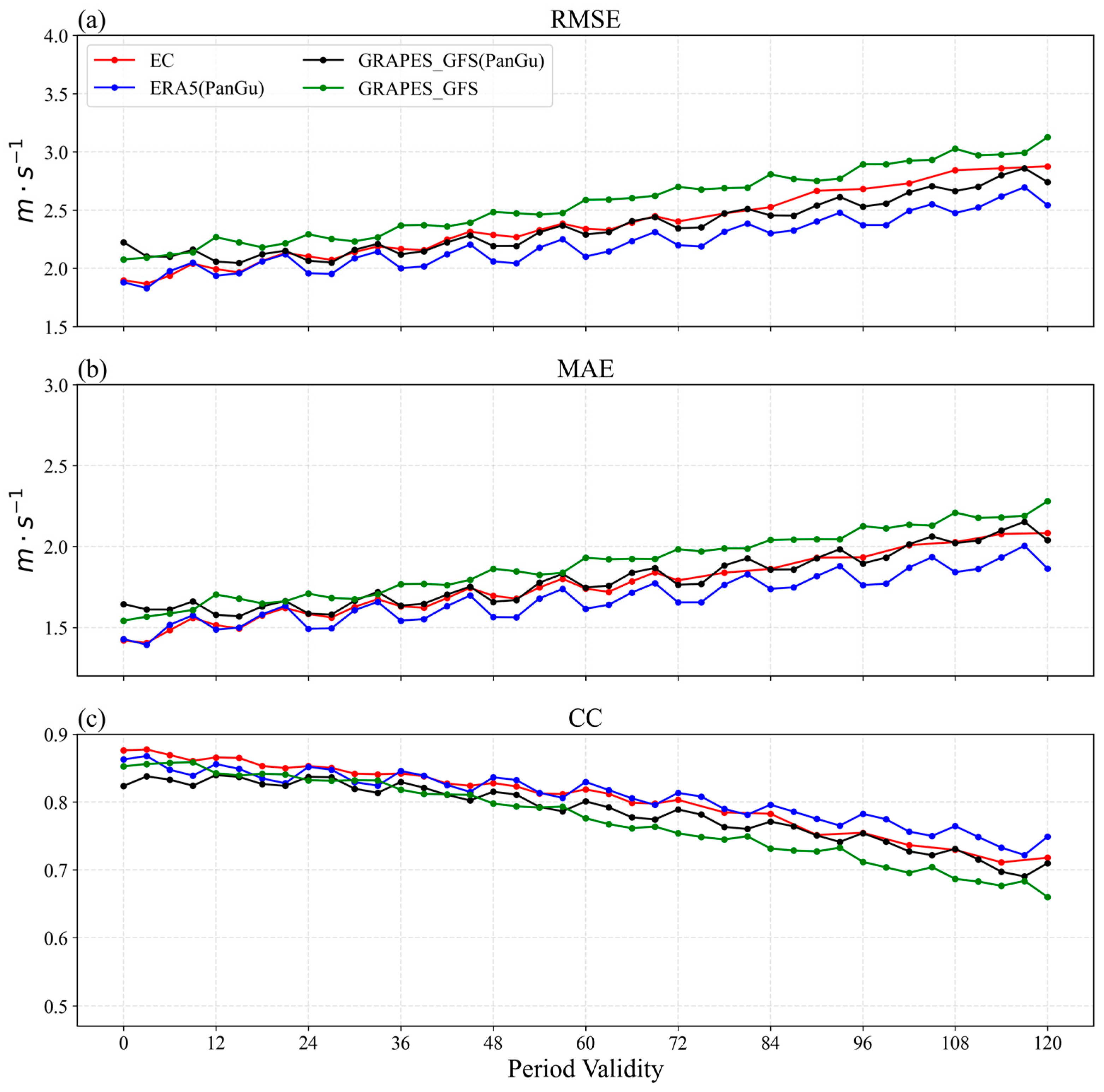
3.1. Wind Speed Comparison and Evaluation

Firstly, the wind speed from buoy observations is used to compare and evaluate the wind speed forecasts under different forecast lead times for the four groups. Figure 2 illustrates the variations in wind speed forecast errors (RMSE, MAE) and correlation coefficients (CCs) with the forecast lead time for the four different forecasts. Overall, the forecast errors for wind speed from the four different forecasting models exhibit a fluctuating increase with the growth in forecast lead time. Additionally, the CCs between forecasted wind speed and observed wind speed decrease as the forecast lead time increases. During the period of 0 h to 60 h, the decrease in the CCs for the four forecast experiments is relatively consistent. This indicates that the consistency between the forecast values and the observed values is generally good for all four forecasting experiments within the first 60 h. The GRAPES_GFS (green line) consistently exhibits higher RMSE and MAE values than the other three experiments within the forecast lead time of 0 h to 120 h. The RMSE ranges from 2.076 m/s to 3.126 m/s, and the MAE ranges from 1.543 m/s to 2.281 m/s. Conversely, the ERA5 (PanGu) (blue line) exhibits the lowest RMSE and MAE values consistently within the forecast lead time of 0 h to 120 h among the four forecast experiments. The RMSE ranges from 1.830 m/s to 2.696 m/s, and the MAE ranges from 1.393 m/s to 2.006 m/s. After 60 h, the CCs remain the highest compared to the other three forecast experiments, indicating the best forecast stability [33] among the four forecast experiments.
In addition to intuitively revealing the overall forecasting performance of the four forecasting experiments, Figure 2 highlights three more detailed aspects.
  • First, examining the initial fields of the GRAPES_GFS (green line) and GRAPES_GFS (PanGu) (black line) experiments, it is evident that the forecast errors in wind speed differ between them. This discrepancy arises because the GRAPES_GFS data are on a grid of 0.125° × 0.125°. Before being used in the PanGu model experiments, the data must be interpolated to a 0.25° × 0.25° grid, introducing interpolation errors. However, when the forecast lead time is between 0 and 3 h, the black line shows a reduction, and at 3, 6, and 9 h, the green and black lines gradually converge. This indicates that the PanGu model has a certain degree of correction capability and demonstrates strong adaptability.
  • Second, compare the GRAPES-GFS (green line) and GRAPES_GFS (PanGu) (black line) experiments, as well as the EC (red line) and ERA5 (PanGu) (blue line) experiments. It is observed that the forecasting error of GRAPES_GFS (PanGu) is lower than that of GRAPES_GFS, and ERA5 (PanGu) exhibits a lower forecasting error compared to EC. This result indicates that the PanGu model, as an advanced intelligent forecasting model, not only outperforms traditional models in forecast response speed but also provides better forecast results compared to conventional NWP (relative to the input NWP).
  • Third, by examining the GRAPES_GFS (green line) and ERA5 (PanGu) (blue line) experiments, it is noted that the latter benefits from a superior initial field. Consequently, during the forecast period of 0–120 h, ERA5 (PanGu) demonstrates smaller wind speed forecast errors and better forecast performance. This comparison underscores that a superior initial field enhances the PanGu model’s forecasting accuracy. Therefore, improving assimilation techniques to construct an initial field with reduced observational errors could further enhance the forecasting performance of the PanGu model.
The Taylor diagram (Figure 3) also reflects the same results. Analyzing and organizing the Taylor diagram, the variations in the standard deviation of wind speed near the Taiwan Strait with forecast lead time for the four forecast experiments are shown in Table 1. The values closest to REF are highlighted in bold. Unlike the RMSE, the standardized variance reflects the degree of dispersion between the forecast values and observations. Using the REF radius as a reference, the four sets of experiments, ranked by their distance from REF from largest to smallest, are EC, GRAPES_GFS, ERA5 (PanGu), and GRAPES_GFS (PanGu). It is evident that despite being model forecasts, the wind speed fluctuations in GRAPES_GFS are less pronounced compared to EC, resulting in a standard deviation closer to REF. Although EC has more accurate forecasts at each time step compared to GRAPES_GFS, it exhibits larger deviations in extreme wind speeds, leading to greater fluctuation levels. The results from the PanGu model also demonstrate that the forecast standard deviation is closer to REF compared to the NWP, indicating that the forecast values are more aligned with the observations. Additionally, GRAPES_GFS (PanGu) being closer to REF than ERA5 (PanGu) further confirms the direct impact of the initial field on forecasts within the PanGu model.
Furthermore, we analyzed the spatial distribution of forecast errors for the four forecast experiments (Figure 4), where data points represent the relative locations of observations, and different colors represent the group with the minimum RMSE for that forecast time step. For instance, when the forecast lead time is 24 h, four sets of experiments are conducted, each represented by a different color. For a specific buoy location, the RMSE is calculated for each experimental set, and the experiment corresponding to the minimum RMSE is identified as experiment (a). Subsequently, the buoy location is marked with the color associated with experiment (a). At different forecast times, the ERA5 (PanGu) forecast has the smallest RMSE for wind speed for the majority of points, accounting for 61.90%, 57.14%, 76.19%, and 66.67%, and 85.71%. This indicates that spatially, the ERA5 (PanGu) has a better forecast performance for the absolute majority of regions among the four forecasts, and as the forecast lead time increases, it covers more areas with better forecast performance. For all locations near the coast of Taiwan, the PanGu model does not achieve a universally superior forecasting performance at every point. For example, as shown in Figure 4a, there are four locations along the Taiwan coast where the EC forecasts perform better. Similarly, Figure 4b indicates that the EC outperforms at three locations, while GRAPES_GFS is superior at two locations. However, in the open ocean regions away from land, the PanGu model consistently provides better forecasts across all lead times. Therefore, considering the inherent difficulty of forecasting coastal and land-sea breezes [34], the PanGu model does not yet exhibit absolute superiority in coastal regions near land. Nonetheless, it demonstrates a stable spatiotemporal forecasting advantage in the open sea areas.

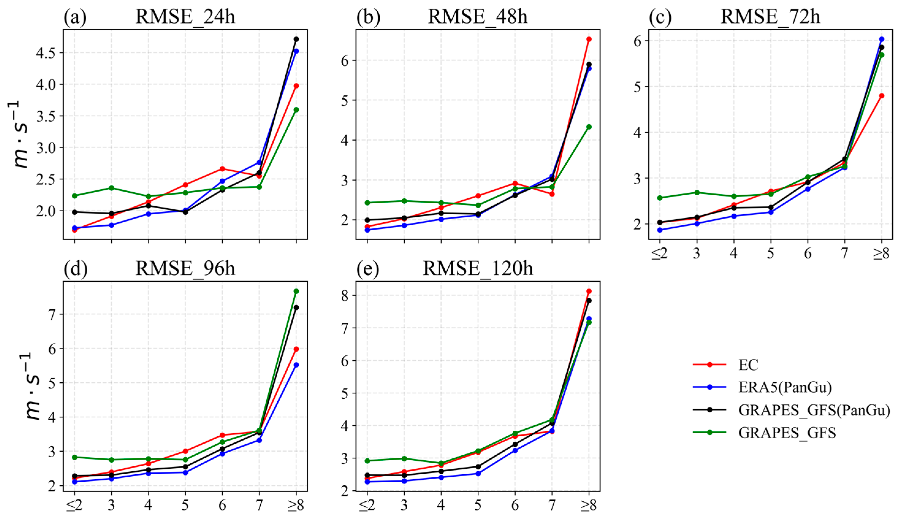
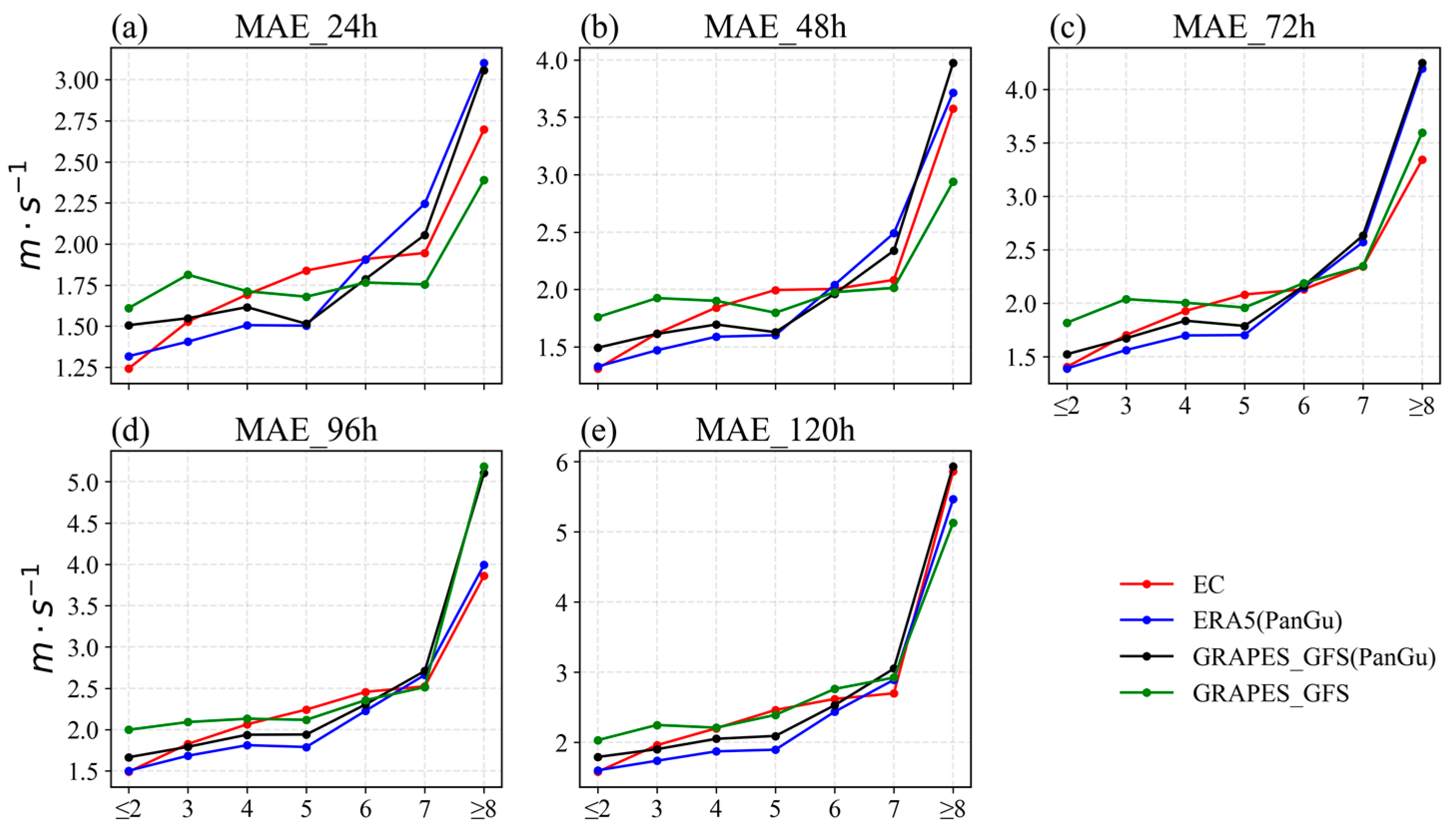
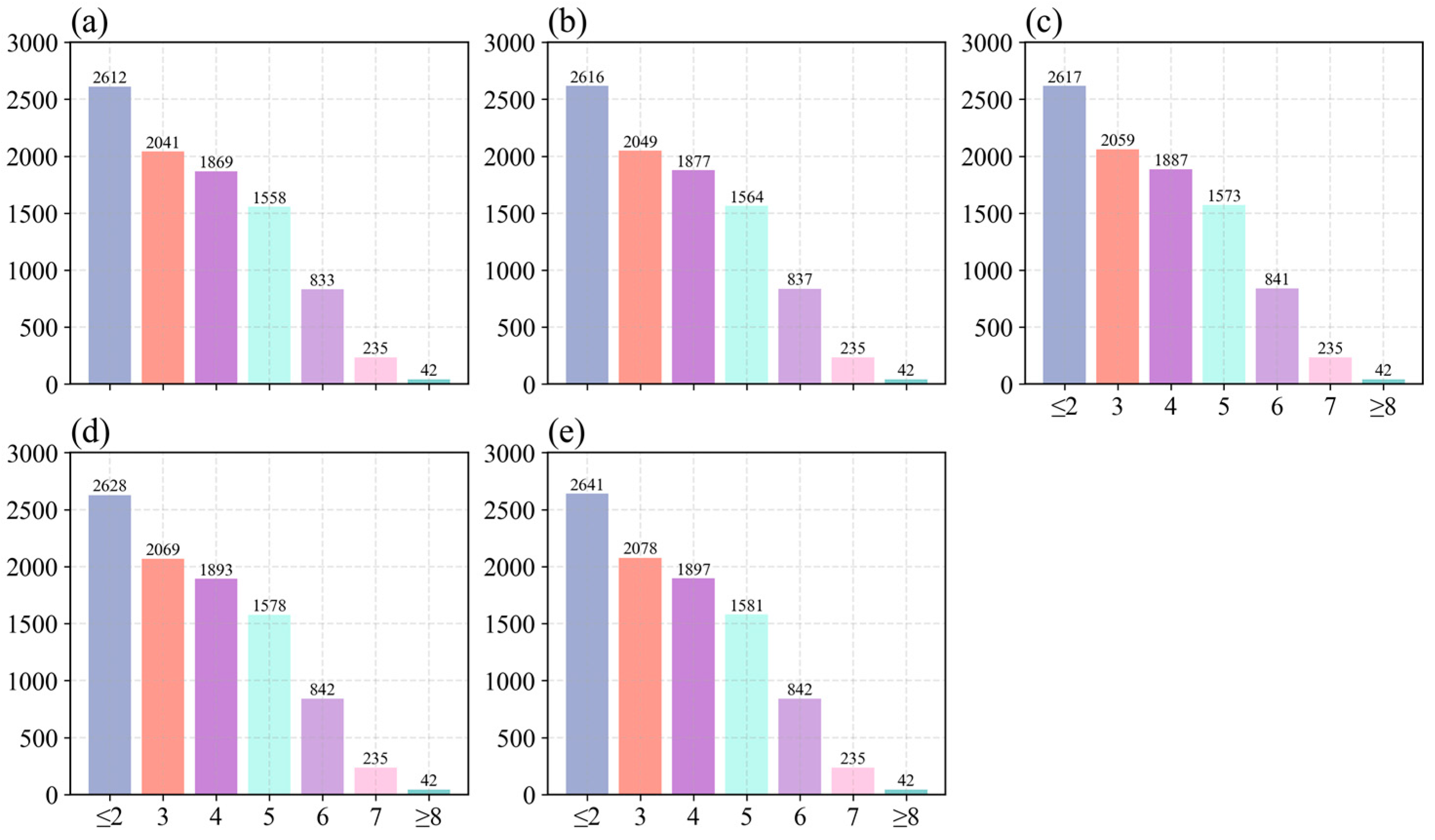
3.2. Wind Speed Level Comparison Evaluation

Traditional wind speed forecasts also categorize wind speeds into different levels. Therefore, in this study, all wind speed data were classified into levels based on the international Beaufort scale standards, combined with the data used in this paper. The wind speeds were divided into seven levels, ≤2, 3, 4, 5, 6, 7, and ≥8.
For forecast intervals of 24 h, 48 h, 72 h, 96 h, and 120 h, the wind speed level RMSE and MAE are shown in Figure 5 and Figure 6. It can be observed that for the five different forecast lead times, ERA5 (PanGu) generally exhibits the best overall forecast performance among the four forecast experiments. The blue line representing ERA5 (PanGu) is consistently at the lowest position among the seven-level categories. Next is GRAPES_GFS (PanGu), which shows a forecast performance only slightly below ERA5 (PanGu).
For wind speed forecasts below level 5, the PanGu model consistently demonstrates superior performance across different initial input fields. Throughout various forecast lead times, the RMSE of the PanGu model fluctuates between 1.725 m/s and 2.739 m/s, while the MAE remains stable between 1.317 m/s and 2.092 m/s. In contrast, the EC model shows a slightly better performance than GRAPES_GFS (PanGu) for wind speeds below level 3, but its forecast errors increase significantly with higher wind levels. Although GRAPES_GFS exhibits a slower increase in wind speed errors with rising wind levels, its overall forecast performance for wind speeds below level 5 is the poorest among the four forecasting experiments.
The forecasting of wind speeds at level 6 appears to be a critical point across the four forecast experiments. For wind speeds below level 6, comparing GRAPES_GFS (green line) and GRAPES_GFS (PanGu) (black line), GRAPES_GFS (PanGu) consistently shows smaller values for both RMSE and MAE. Moreover, the RMSE and MAE for GRAPES_GFS (PanGu) (black line) and ERA5 (PanGu) (blue line) show minimal differences and similar trends for wind speeds below level 6, indicating the operational transferability of the PanGu model in smaller regions.
For wind speed forecasts at level 8 or above, all four forecast experiments show varying degrees of rapid error growth. Furthermore, for different lead times, the PanGu model generally performs worse than the NWP. Thus, the PanGu model does not excel in forecasting high wind speeds (i.e., wind speed levels ≥ 8). However, due to the large forecast errors for wind speeds ≥ 8 across all four experiments, we analyzed the number of valid samples for different wind levels and lead times (i.e., the amount of data from buoy observations), as shown in Figure 7. It is evident that for wind speed levels ≥ 8, the number of valid data points is less than 50. Since RMSE and MAE are types of average statistical measures, the amount of data can influence the final results to some extent. Therefore, when the total data volume for wind speed levels ≥ 8 is very small, the reliability of the wind speed assessment for these levels is reduced. In short, the overall trends of the four forecast experiments follow the general pattern of wind speed forecasts. The results are highly credible for wind speed levels ≤ 7, and the PanGu weather prediction model performs better than others in the same category of forecasts.

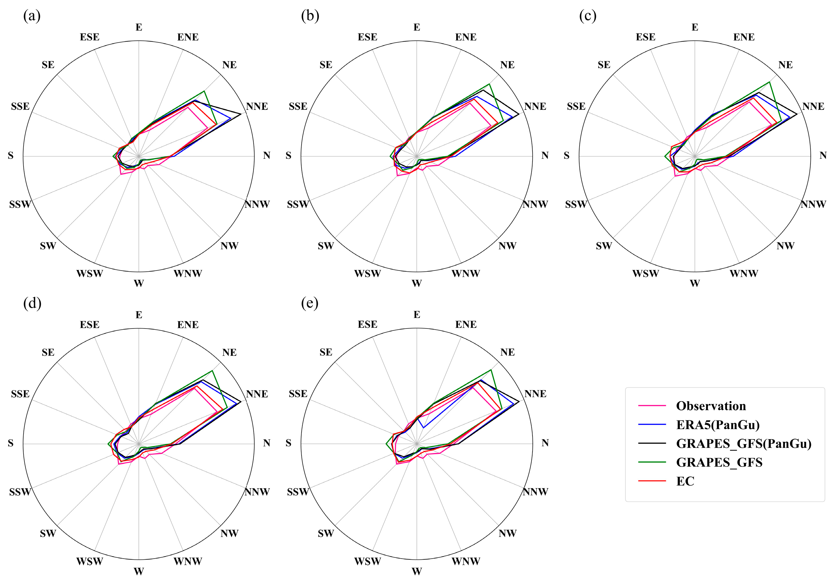
3.3. Wind Direction Comparative Evaluation

In addition to wind speed forecasts, wind direction is equally crucial. Figure 8 illustrates the variation in wind direction forecast errors for different forecast experiments over forecast lead times. From the figure, it can be observed that both the RMSE and MAE for wind direction forecasts exhibit a fluctuating upward trend with increasing forecast lead times.
When the forecast lead time exceeds 48 h, the RMSE and MAE of the PanGu weather forecasting model gradually become smaller than those of the GRAPES_GFS model but still fall short of the results from the EC model. Overall, the EC model demonstrates better control over wind direction forecasts; however, it also exhibits a faster increase in RMSE and MAE as the forecast lead time extends. The PanGu weather forecasting model, on the other hand, better demonstrates its advantage in stability for forecast lead times greater than 48 h.
In the process of wind energy development, wind direction frequency is also a crucial factor. Having one or two dominant wind directions significantly enhances the efficiency of wind turbines, making the accurate forecasting of dominant wind directions a key aspect of wind field forecasting. Figure 9 reflects the wind direction frequencies at different forecast lead times, showing that the Taiwan Strait area predominantly experiences northeast (NE) and north–northeast (NNE) winds. All four forecasting experiments show a higher frequency of NE and NNE winds, with good accuracy for low-frequency wind directions. The PanGu weather forecasting model shows less accuracy for NNE wind forecasts compared to model forecasts but performs better than GRAPES_GFS and slightly worse than EC for NE winds. Overall, while the EC model’s forecasts are closer to the observation field results, the PanGu weather forecasting model also provides relatively accurate and rapid forecasts of the main wind directions within a shorter time frame, which is of significance for coastal wind turbine construction.

4. Conclusions and Discussion

This study evaluated 10 m wind forecasts in the Taiwan Strait region using buoy observation data, comparing forecasts from the EC high-resolution grid, GRAPES-GFS, and two PanGu weather model experiments initialized with ERA5 reanalysis data and GRAPES-GFS analysis data, respectively. The main conclusions drawn are as follows:
  • Performance Comparison:
Compared to numerical forecasts, the PanGu weather model-based forecasts exhibit better performance in predicting 10 m wind fields. Over forecast lead times of 0–120 h, the PanGu weather model forecasts show higher correlation coefficients and smaller forecast errors with buoy observations compared to the numerical forecasts. The Taylor diagrams further confirm this. Spatially, the PanGu weather model forecasts have fewer points with smaller wind speed errors compared to numerical forecasts, indicating better predictive performance for local 10 m wind speed distributions.
For different wind speed levels, all four forecast experiments show relatively small forecast errors for wind speeds of 2–7 m/s. The PanGu weather model exhibits smaller forecast errors for different wind speed levels than the numerical models. However, all forecast experiments show significant errors for high wind speeds (wind speed > 7 m/s), possibly due to limited sample data for high wind forecasts.
The differences among the four forecast experiments are relatively small for low-frequency wind direction forecasts, while the EC model’s forecasts are closer to the observation field results. However, the PanGu weather forecasting model also provides relatively accurate and rapid forecasts of the main wind directions within a shorter time frame, which is of significance for coastal wind turbine construction.
  • Initialization Comparison:
The PanGu weather model initialized with ERA5 data performs better in forecasting 10 m wind fields compared to the one initialized with the GRAPES-GFS analysis data. ERA5 data provide a smaller initial wind speed error compared to GRAPES-GFS analysis data, resulting in lower RMSE (1.88 m/s) and MAE (1.428 m/s) for 10 m wind speed forecasts. This indicates that a more suitable initial field leads to better forecast results for the PanGu weather model.
In conclusion, this study confirms that the PanGu weather model outperforms traditional numerical forecasts in predicting 10 m wind fields in the Taiwan Strait region from 1 June 2023 to 31 May 2024. However, further evaluations are needed to determine if similar conclusions apply to other periods and regions.
Additionally, the current research indicates that traditional numerical methods still outperform intelligent forecasting models in forecast accuracy before the introduction of the PanGu model [35,36]. However, the advent of the PanGu model signifies the first instance where AI-based forecasting models have surpassed traditional numerical methods in both accuracy and speed. We hypothesize several reasons for this development:
  • Despite the lack of physical interpretability in using deep learning for weather forecasting [14,37], its initial proposition highlighted its powerful capability to fit nonlinear equations given ample data [38]. Numerical weather prediction fundamentally involves solving a set of partial differential equations (e.g., thermodynamic equations, N-S equations) starting from initial atmospheric conditions to simulate various physical processes [12,39]. Thus, the PanGu model, trained on 39 years of ERA5 data, can feasibly learn nonlinear relationships among atmospheric variables and has demonstrated transferability using GRAPES_GFS data.
  • Bi et al. [27] identified two primary reasons why previous intelligent weather forecasting models have exhibited lower accuracy compared to traditional numerical models: (i) Weather forecasting necessitates consideration of high dimensions. Atmospheric relationships vary rapidly among different pressure levels, and atmospheric distributions across pressure levels are non-uniform. Previous two-dimensional intelligent weather forecasting models [40,41,42] struggle with rapid changes across different pressure levels. Additionally, many weather processes (e.g., radiation, convection) can only be fully described in three-dimensional space, which two-dimensional models cannot effectively utilize. (ii) When models are iteratively invoked, iterative errors accumulate. Intelligent forecasting models, lacking constraints from partial differential equations, experience super-linear growth in iterative errors over time.
The above discussion represents our initial conjectures about the better forecast performance of PanGu. The detailed reasons behind the PanGu weather model’s superior performance warrant further investigation in future research.

Author Contributions

Conceptualization, J.Y. (Jun Yi) and X.L.; methodology, X.L. and Y.Z.; software, X.L. and Y.Z.; validation, J.Y. (Jun Yi), X.L. and J.Y. (Jiawei Yao); formal analysis, J.Y. (Jun Yi); data curation, X.L., J.Y. (Jiawei Yao), H.Q. and K.Y.; writing—original draft preparation, J.Y. (Jun Yi); writing—review and editing, J.Y. (Jun Yi), X.L. and Y.Z.; visualization, J.Y. (Jun Yi); supervision, X.L. and Y.Z.; All authors have read and agreed to the published version of the manuscript.

Funding

The National Key Research and Development Program of China (2023YFC3008005). The National Natural Science Foundation of China (No. 42375062). The Research Project of China Three Gorges Corporation (No. 202103460).

Institutional Review Board Statement

Not applicable.

Informed Consent Statement

Not applicable.

Data Availability Statement

The data presented in this study are available on request from the corresponding author due to privacy.

Acknowledgments

We are very grateful for the comments from anonymous reviewers who have helped us improve the quality of this article.

Conflicts of Interest

Author Kan Yi was employed by the company China Three Gorges Corporation. The remaining authors declare that the research was conducted in the absence of any commercial or financial relationships that could be construed as a potential conflict of interest.

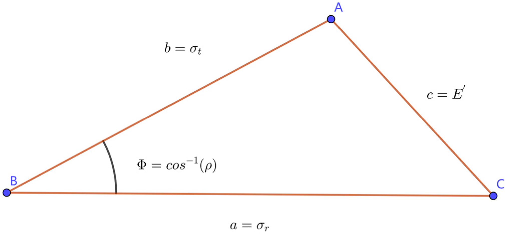
Appendix A. Introduction to Taylor Diagram

Taylor diagrams are mathematical charts for comparing standard deviations, root mean square errors, and correlations. They were invented by Karl Taylor in 1994 to evaluate the accuracy of model simulations and illustrate the degree of agreement between models [43]. According to the error propagation formula, the three statistical quantities shown in Taylor diagrams can be intuitively understood based on the cosine theorem (Figure A1), expressed as follows:
c 2 = a 2 + b 2 2 ab cos Φ
where c represents the root mean square error between the observed field and the simulated field; a represents the standard deviation of the observed field; b represents the standard deviation of the simulated field; and the cosine of the angle Φ between a and b is the correlation coefficient.
Figure A1. The geometric relationship between statistical parameters on the Taylor diagram is illustrated based on the cosine theorem [43].
Atmosphere 15 00977 g0a1
In the Taylor diagram, the values on the axes corresponding to the arcs centered at the origin represent the ratio of the spatial variability standard deviation of the model simulation to that of the observation. The values on the major arcs corresponding to each point represent the spatial correlation coefficient between the model and the observation. The distances between each point and the REF reference point (reference field) represent the root mean square error.

References

  1. Qu, H.; Huang, B.; Zhao, W.; Song, J.; Guo, Y.; Hu, H.; Cao, Y. Comparison and evaluation of HRCLDAS-V1.0 and ERA5 sea-surface wind fields. J. Trop. Meteorol. 2022, 38, 569–579. [Google Scholar]
  2. Fan, K.; Xu, Q.; Xu, D.; Xie, R.; Ning, J.; Huang, J. Review of remote sensing of sea surface wind field by space-borne SAR. Prog. Geophys. 2022, 37, 1807–1817. [Google Scholar]
  3. Stammer, D.; Wunsch, C.; Giering, R.; Eckert, C.; Heimbach, P.; Marotzke, J.; Adcroft, A.; Hill, C.N.; Marshall, J. Global Ocean Circulation during 1992–1997, Estimated from Ocean Observations and a General Circulation Model. J. Geophys. Res. Ocean 2002, 107, 1-1–1-27. [Google Scholar] [CrossRef]
  4. Kim, E.; Manuel, L.; Curcic, M.; Chen, S.S.; Phillips, C.; Veers, P. On the Use of Coupled Wind, Wave, and Current Fields in the Simulation of Loads on Bottom-Supported Offshore Wind Turbines during Hurricanes: March 2012–September 2015; NREL/TP--5000-65283; NREL/TP: Golden, CO, USA, 2016.
  5. Veers, P.; Dykes, K.; Lantz, E.; Barth, S.; Bottasso, C.L.; Carlson, O.; Clifton, A.; Green, J.; Green, P.; Holttinen, H.; et al. Grand Challenges in the Science of Wind Energy. Science 2019, 366, eaau2027. [Google Scholar] [CrossRef] [PubMed]
  6. Worsnop, R.P.; Lundquist, J.K.; Bryan, G.H.; Damiani, R.; Musial, W. Gusts and Shear Within Hurricane Eyewalls Can Exceed Offshore Wind-Turbine Design Standards. Geophys. Res. Lett. 2017, 44, 6413–6420. [Google Scholar] [CrossRef]
  7. Li, M.; Wang, H.; Jin, Q. A review on the forecast method of China offshore wind. Mar. Forecast. 2009, 26, 114–120. [Google Scholar]
  8. Chen, X.; Hao, Z.; Pan, D.; Huang, S.; Gong, F.; Shi, D. Analysis of temporal and spatial feature of sea surface wind field in China offshore. J. Mar. Sci. 2014, 32, 1–10. [Google Scholar]
  9. Zheng, C. Sea surface wind field analysis in the China sea during the last 22 years with CCMP wind field. Meteorol. Disaster Reduct. Res. 2011, 34, 41–46. [Google Scholar]
  10. Zhang, J.; Zhu, X. Verification of prediction capability of NWP products and objective forecast methods. Meteorol. Mon. 2006, 32, 58–63. [Google Scholar]
  11. Yang, C.; Zheng, Y.; Lin, J.; Li, F. Numerical model output validation and assessment. J. Meteorol. Res. Appl. 2008, 29, 32–37. [Google Scholar]
  12. Bauer, P.; Thorpe, A.; Brunet, G. The Quiet Revolution of Numerical Weather Prediction. Nature 2015, 525, 47–55. [Google Scholar] [CrossRef] [PubMed]
  13. de Bezenac, E.; Pajot, A.; Gallinari, P. Deep Learning for Physical Processes: Incorporating Prior Scientific Knowledge. J. Stat. Mech. Theory Exp. 2019, 2019, 124009. [Google Scholar] [CrossRef]
  14. Reichstein, M.; Camps-Valls, G.; Stevens, B.; Jung, M.; Denzler, J.; Carvalhais, N. Prabhat Deep Learning and Process Understanding for Data-Driven Earth System Science. Nature 2019, 566, 195–204. [Google Scholar] [CrossRef]
  15. Lydia, M.; Kumar, G.E.P. Deep Learning Algorithms for Wind Forecasting: An Overview. In Artificial Intelligence for Renewable Energy Systems; Vyas, A.K., Balamurugan, S., Hiran, K.K., Dhiman, H.S., Eds.; Wiley: Hoboken, NJ, USA, 2022; pp. 129–145. [Google Scholar]
  16. Lin, Z.; Liu, X. Wind Power Forecasting of an Offshore Wind Turbine Based on High-Frequency SCADA Data and Deep Learning Neural Network. Energy 2020, 201, 117693. [Google Scholar] [CrossRef]
  17. Cheng, L.; Zang, H.; Ding, T.; Sun, R.; Wang, M.; Wei, Z.; Sun, G. Ensemble Recurrent Neural Network Based Probabilistic Wind Speed Forecasting Approach. Energies 2018, 11, 1958. [Google Scholar] [CrossRef]
  18. Wang, G.; Wang, X.; Hou, M.; Qi, Y.; Song, J.; Liu, K.; Wu, X.; Bai, Z. Research on application of LSTM deep neural network on historical observation data and reanalysis data for sea surface wind speed forecasting. Haiyang Xuebao 2020, 42, 67–77. [Google Scholar]
  19. Liu, X.; Zhang, H.; Kong, X.; Lee, K.Y. Wind Speed Forecasting Using Deep Neural Network with Feature Selection. Neurocomputing 2020, 397, 393–403. [Google Scholar] [CrossRef]
  20. Ju, Y.; Sun, G.; Chen, Q.; Zhang, M.; Zhu, H.; Rehman, M.U. A Model Combining Convolutional Neural Network and LightGBM Algorithm for Ultra-Short-Term Wind Power Forecasting. IEEE Access 2019, 7, 28309–28318. [Google Scholar] [CrossRef]
  21. Lam, R.; Sanchez-Gonzalez, A.; Willson, M.; Wirnsberger, P.; Fortunato, M.; Alet, F.; Ravuri, S.; Ewalds, T.; Eaton-Rosen, Z.; Hu, W.; et al. Learning Skillful Medium-Range Global Weather Forecasting. Science 2023, 382, 1416–1421. [Google Scholar] [CrossRef]
  22. Kurth, T.; Subramanian, S.; Harrington, P.; Pathak, J.; Mardani, M.; Hall, D.; Miele, A.; Kashinath, K.; Anandkumar, A. FourCastNet: Accelerating Global High-Resolution Weather Forecasting Using Adaptive Fourier Neural Operators. In Proceedings of the Platform for Advanced Scientific Computing Conference, Davos, Switzerland, 26–28 June 2023; ACM: Davos, Switzerland, 2023; pp. 1–11. [Google Scholar]
  23. Zhang, Y.; Long, M.; Chen, K.; Xing, L.; Jin, R.; Jordan, M.I.; Wang, J. Skilful Nowcasting of Extreme Precipitation with NowcastNet. Nature 2023, 619, 526–532. [Google Scholar] [CrossRef] [PubMed]
  24. Hu, Y.; Chen, L.; Wang, Z.; Li, H. SwinVRNN: A Data-Driven Ensemble Forecasting Model via Learned Distribution Perturbation. J. Adv. Model. Earth Syst. 2023, 15, e2022MS003211. [Google Scholar] [CrossRef]
  25. Chen, L.; Zhong, X.; Zhang, F.; Cheng, Y.; Xu, Y.; Qi, Y.; Li, H. FuXi: A Cascade Machine Learning Forecasting System for 15-Day Global Weather Forecast. Clim. Atmos. Sci. 2023, 6, 190. [Google Scholar] [CrossRef]
  26. Chen, K.; Han, T.; Gong, J.; Bai, L.; Ling, F.; Luo, J.-J.; Chen, X.; Ma, L.; Zhang, T.; Su, R.; et al. FengWu: Pushing the Skillful Global Medium-Range Weather Forecast beyond 10 Days Lead. arXiv 2023, arXiv:2304.02948. [Google Scholar]
  27. Bi, K.; Xie, L.; Zhang, H.; Chen, X.; Gu, X.; Tian, Q. Accurate Medium-Range Global Weather Forecasting with 3D Neural Networks. Nature 2023, 619, 533–538. [Google Scholar] [CrossRef]
  28. Zhang, Y. Evaluation of three reanalysis surface wind products in Taiwan Strait. J. Fish. Res. 2020, 42, 556–571. [Google Scholar]
  29. Pan, W.; Lin, Y. Spatial feature and seasonal variability characteristics of sea surface wind field in Taiwan Strait from 2007 to 2017. J. Trop. Meteorol. 2019, 35, 296–303. [Google Scholar]
  30. Han, Y.; Zhou, L.; Zhao, Y.; Jiang, H.; Yu, D. Evaluation of three sea surface wind data sets in Luzon Strait. Mar. Forecast. 2019, 36, 44–52. [Google Scholar]
  31. Kalverla, P.; Steeneveld, G.; Ronda, R.; Holtslag, A.A. Evaluation of Three Mainstream Numerical Weather Prediction Models with Observations from Meteorological Mast IJmuiden at the North Sea. Wind Energy 2019, 22, 34–48. [Google Scholar] [CrossRef]
  32. Wang, Z.; Xu, X.; Xiong, N.; Yang, L.T.; Zhao, W. GPU Acceleration for GRAPES Meteorological Model. In Proceedings of the 2011 IEEE International Conference on High Performance Computing and Communications, Banff, AB, Canada, 2–4 September 2011; IEEE: Piscataway, NJ, USA, 2011; pp. 365–372. [Google Scholar]
  33. Pappenberger, F.; Cloke, H.L.; Persson, A.; Demeritt, D. HESS Opinions “On forecast (in)consistency in a hydro-meteorological chain: Curse or blessing?”. Hydrol. Earth Syst. Sci. 2011, 15, 2391–2400. [Google Scholar] [CrossRef]
  34. Case, J.L.; Wheeler, M.M.; Merceret, F.J. Final Report on Land-Breeze Forecasting; NASA Technical Reports Server. Available online: https://kscweather.ksc.nasa.gov/amu/files/final-reports/landbreeze.pdf (accessed on 1 June 2024).
  35. Weyn, J.A.; Durran, D.R.; Caruana, R. Can Machines Learn to Predict Weather? Using Deep Learning to Predict Gridded 500-hPa Geopotential Height From Historical Weather Data. J. Adv. Model. Earth Syst. 2019, 11, 2680–2693. [Google Scholar] [CrossRef]
  36. Rasp, S.; Thuerey, N. Data-Driven Medium-Range Weather Prediction with a Resnet Pretrained on Climate Simulations: A New Model for WeatherBench. J. Adv. Model. Earth Syst. 2021, 13, e2020MS002405. [Google Scholar] [CrossRef]
  37. Schultz, M.G.; Betancourt, C.; Gong, B.; Kleinert, F.; Langguth, M.; Leufen, L.H.; Mozaffari, A.; Stadtler, S. Can Deep Learning Beat Numerical Weather Prediction? Philos. Trans. R. Soc. A-Math. Phys. Eng. Sci. 2021, 379, 20200097. [Google Scholar] [CrossRef] [PubMed]
  38. Rumelhart, D.E.; Hinton, G.E.; Williams, R.J. Learning Internal Representations by Error Propagation. In Parallel Distributed Processing. 1: Foundations; Rumelhart, D.E., Mcclelland, J., Eds.; MIT Press: Cambridge, MA, USA, 1999; ISBN 978-0-262-18120-4. [Google Scholar]
  39. Lynch, P. The Origins of Computer Weather Prediction and Climate Modeling. J. Comput. Phys. 2008, 227, 3431–3444. [Google Scholar] [CrossRef]
  40. Rasp, S.; Dueben, P.D.; Scher, S.; Weyn, J.A.; Mouatadid, S.; Thuerey, N. WeatherBench: A Benchmark Data Set for Data-Driven Weather Forecasting. J. Adv. Model. Earth Syst. 2020, 12, e2020MS002203. [Google Scholar] [CrossRef]
  41. Weyn, J.A.; Durran, D.R.; Caruana, R.; Cresswell-Clay, N. Sub-Seasonal Forecasting with a Large Ensemble of Deep-Learning Weather Prediction Models. J. Adv. Model. Earth Syst. 2021, 13, e2021MS002502. [Google Scholar] [CrossRef]
  42. Pathak, J.; Subramanian, S.; Harrington, P.; Raja, S.; Chattopadhyay, A.; Mardani, M.; Kurth, T.; Hall, D.; Li, Z.; Azizzadenesheli, K.; et al. FourCastNet: A Global Data-Driven High-Resolution Weather Model Using Adaptive Fourier Neural Operators. arXiv 2022, arXiv:2202.11214. [Google Scholar]
  43. Taylor, K.E. Summarizing Multiple Aspects of Model Performance in a Single Diagram. J. Geophys. Res. 2001, 106, 7183–7192. [Google Scholar] [CrossRef]
Figure 1. Taiwan Strait buoy observation data point schematic diagram.
Atmosphere 15 00977 g001
Figure 2. Graph depicting the variation in RMSE (a), MAE (b), and CCs (c) of wind speed for four forecasting experiments in the vicinity of the Taiwan Strait: the red line represents the EC grid forecast; the green line represents GRAPES_GFS model forecast; the blue line represents the ERA5 (PanGu) forecast; and the black line represents the GRAPES_GFS (PanGu) forecast.
Atmosphere 15 00977 g002
Figure 3. Taylor diagram showing the variation in wind speed near the Taiwan Strait for four forecasting experiments with forecast lead time; numerical labels correspond to different forecast lead times; red circles represent PanGu forecasts initialized with ERA5; blue asterisks represent PanGu forecasts initialized with GRAPES_GFS; green diamonds represent EC grid forecasts; black stars represent GRAPES_GFS model forecasts. The radial dotted lines are the contour lines of the correlation coefficient; the arc dotted lines are the contour lines of the standard deviation; and the arc solid lines are the contour lines of the central root mean square error compared with the observed value.
Atmosphere 15 00977 g003
Figure 4. Point maps showing the average RMSE of wind speed near the Taiwan Strait for four forecasting experiments at forecast lead times of 24 h (a), 48 h (b), 72 h (c), 96 h (d), and 120 h (e); blue corresponds to PanGu forecasts initialized with ERA5; red corresponds to PanGu forecasts initialized with GRAPES_GFS; green corresponds to EC grid forecasts; yellow corresponds to GRAPES_GFS model forecasts.
Atmosphere 15 00977 g004
Figure 5. Average RMSE plots for wind speed levels of ≤2, 3, 4, 5, 6, 7, and ≥8 near the Taiwan Strait for four forecasting experiments at forecast lead times of 24 h (a), 48 h (b), 72 h (c), 96 h (d), and 120 h (e); the blue line corresponds to PanGu forecasts initialized with ERA5; the black line corresponds to PanGu forecasts initialized with GRAPES_GFS; the red line represents EC grid forecasts; the green line represents GRAPES_GFS model forecasts.
Atmosphere 15 00977 g005
Figure 6. Average MAE plots for wind speed levels of ≤2, 3, 4, 5, 6, 7, and ≥8 near the Taiwan Strait for four forecasting experiments at forecast lead times of 24 h (a), 48 h (b), 72 h (c), 96 h (d), and 120 h (e); the blue line corresponds to PanGu forecasts initialized with ERA5; the black line corresponds to PanGu forecasts initialized with GRAPES_GFS; the red line represents EC grid forecasts; the green line represents GRAPES_GFS model forecasts.
Atmosphere 15 00977 g006
Figure 7. The effective sample size of wind speed for different wind levels (≤2, 3, 4, 5, 6, 7, ≥8) at forecast lead times of 24 h (a), 48 h (b), 72 h (c), 96 h (d), and 120 h (e).
Atmosphere 15 00977 g007
Figure 8. The RMSE (a) and MAE (b) of wind direction for four forecast experiments in the vicinity of the Taiwan Strait within the forecast lead time of 0~120 h. The red line represents the EC forecast, the green line represents the GRAPES_GFS forecast; the blue line represents the ERA5 (PanGu) forecast; and the black line represents the GRAPES_GFS (PanGu) forecast.
Atmosphere 15 00977 g008
Figure 9. Wind direction radar charts for four forecasting experiments in the Taiwan Strait area at forecast lead times of 24 h (a), 48 h (b), 72 h (c), 96 h (d), and 120 h (e). The pink line represents the observation field; the blue line represents the PanGu forecasts initialized with ERA5; the black line represents the PanGu forecasts initialized with GRAPES_GFS; the green line represents the GRAPES_GFS model forecasts; and the red line represents the EC grid forecasts.
Atmosphere 15 00977 g009
Table 1. Variation in the standard deviation of wind speed near the Taiwan Strait for four forecasting experiments with forecast lead time. Unit: (m/s).
Four Sets of Forecasting Experiments24 h48 h72 h96 h120 h
GRAPES_GFS (PanGu)0.9750.9730.9710.9740.970
ERA5 (PanGu)0.9480.9440.9530.9600.957
GRAPES_GFS1.0761.0681.0671.0581.060
EC1.0931.1051.0791.0811.085
Disclaimer/Publisher’s Note: The statements, opinions and data contained in all publications are solely those of the individual author(s) and contributor(s) and not of MDPI and/or the editor(s). MDPI and/or the editor(s) disclaim responsibility for any injury to people or property resulting from any ideas, methods, instructions or products referred to in the content.

