
Generating Daily High-Resolution Regional XCO2 by Deep Neural Network and Multi-Source Data


Abstract
:1. Introduction
2. Data and Method
2.1. Data
- (1)
- OCO-2 XCO2
- (2)
- Carbon Tracker XCO2
- (3)
- CAMS XCO2 and XCH4
- (4)
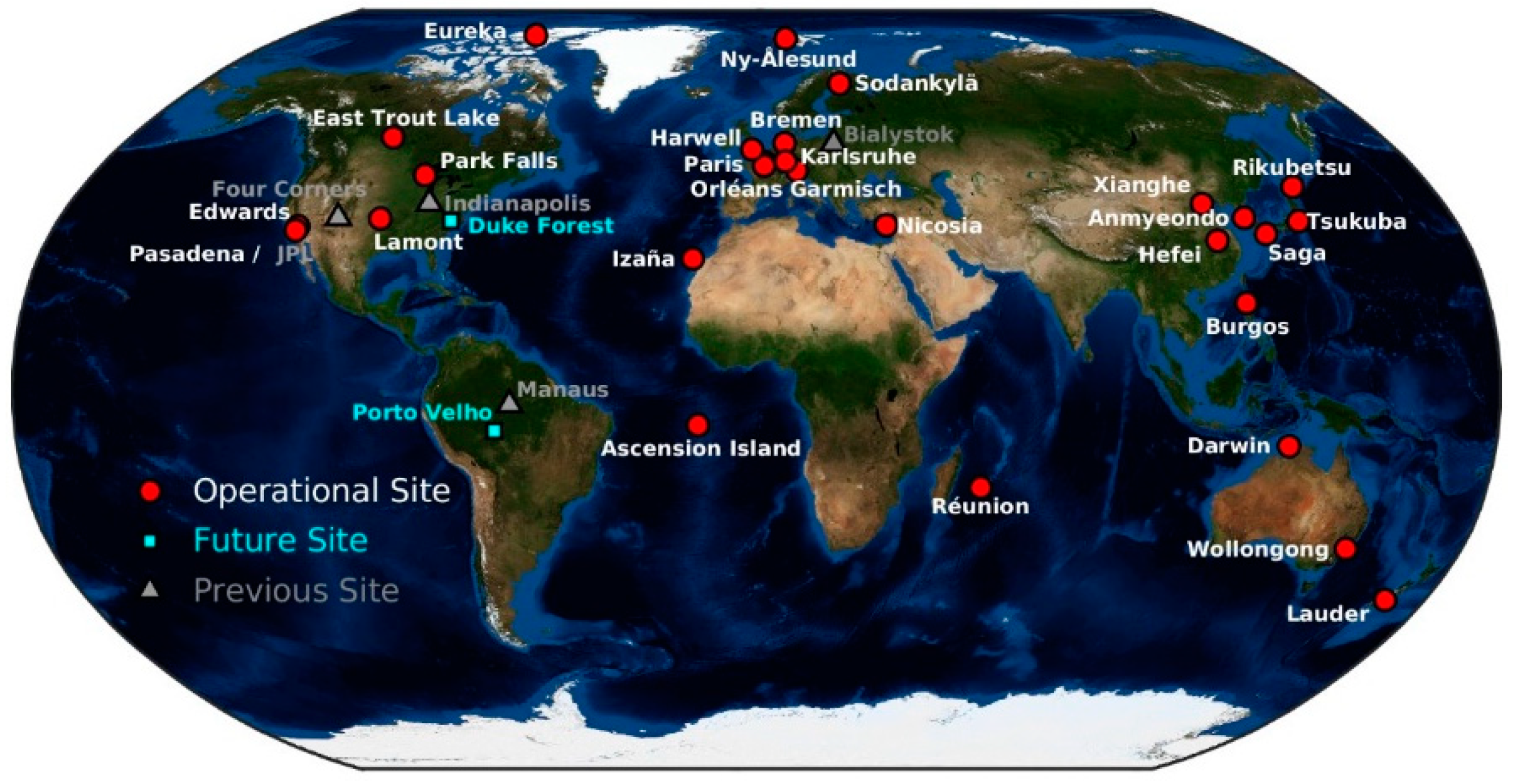
- TCCON XCO2
- (5)
- Vegetation data
- (6)
- Meteorological data
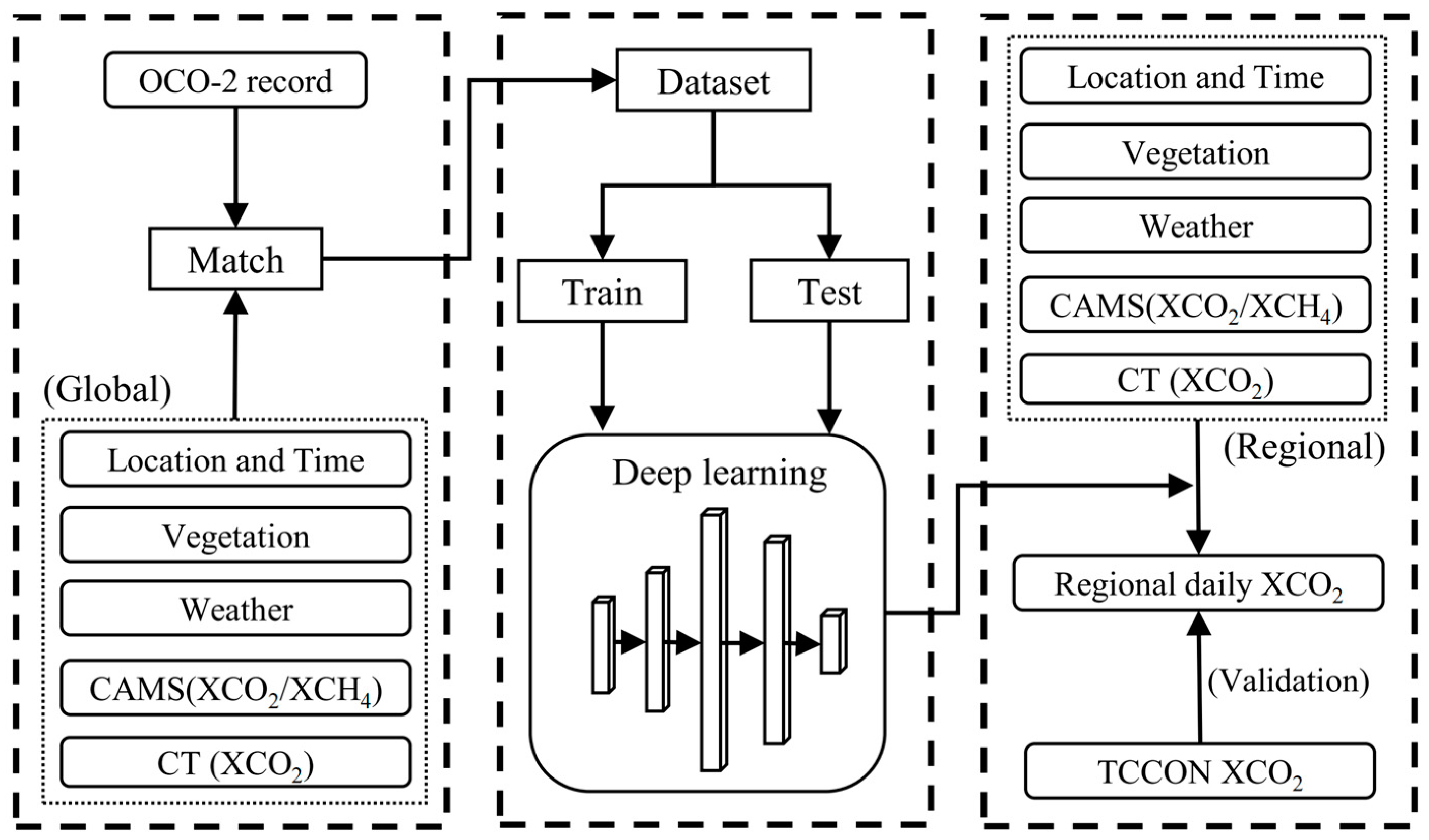
2.2. Method
3. Results and Discussion
3.1. DNN Testing and Accuracy Verification
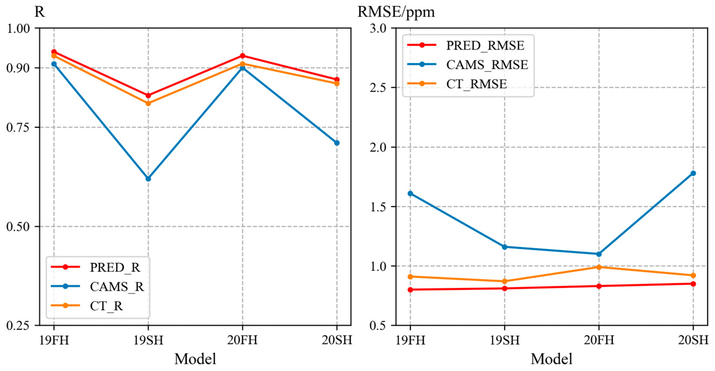
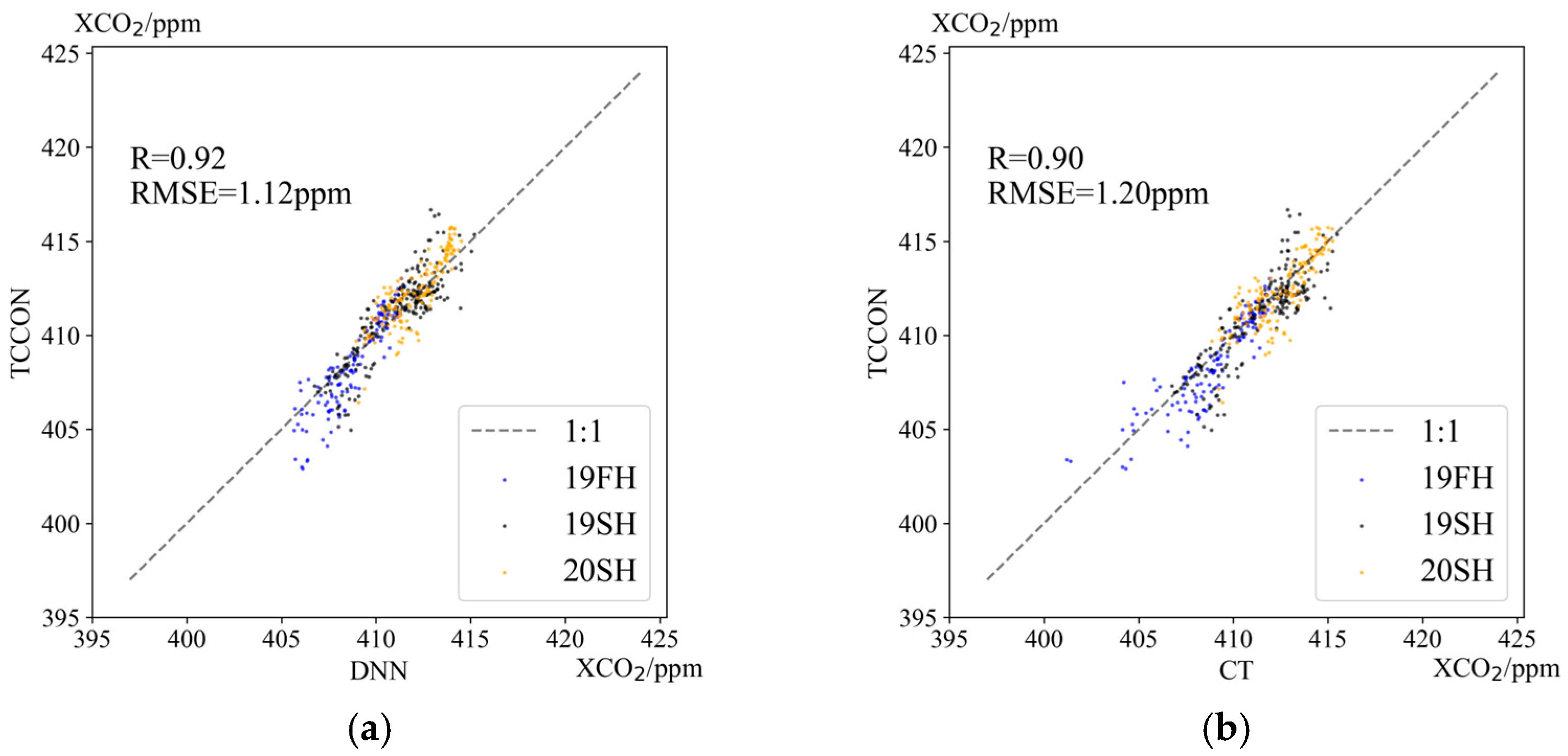
3.2. Performance of Model in Unknown Time
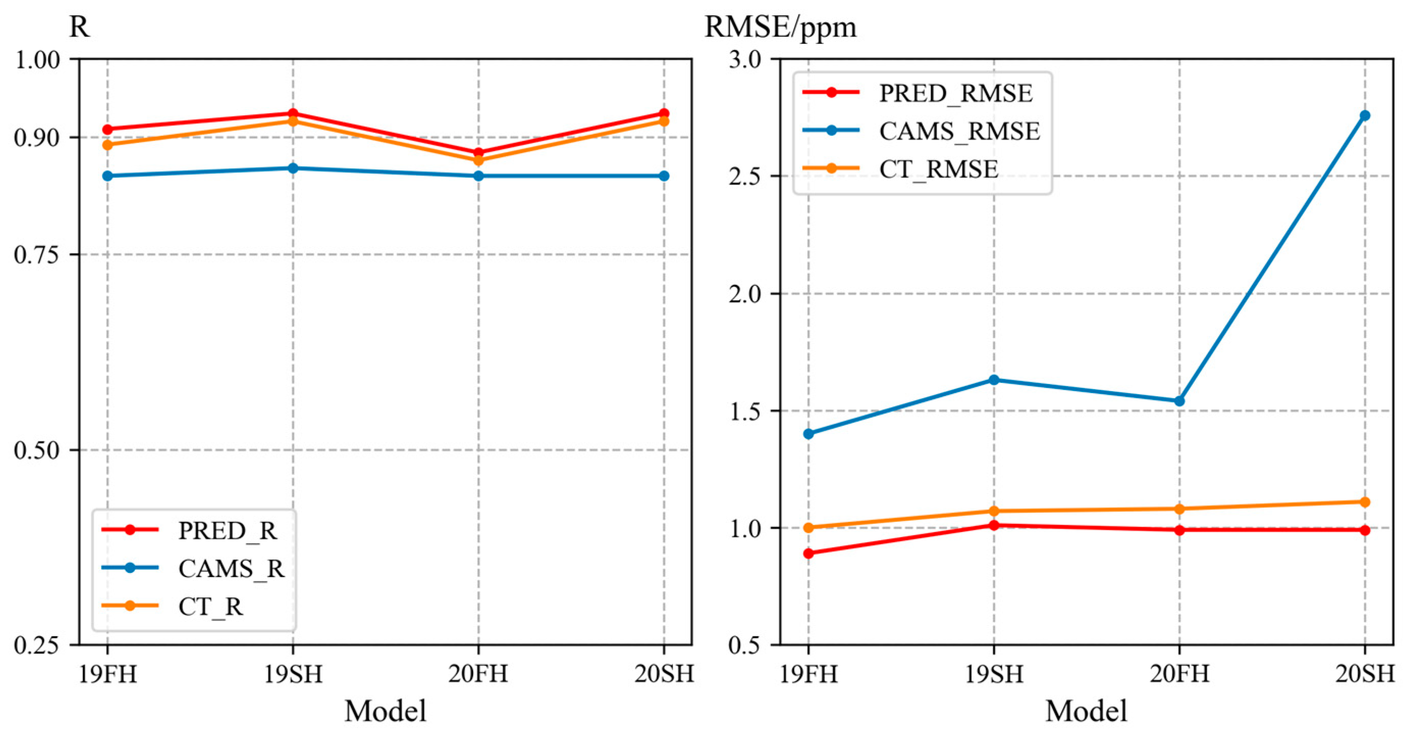
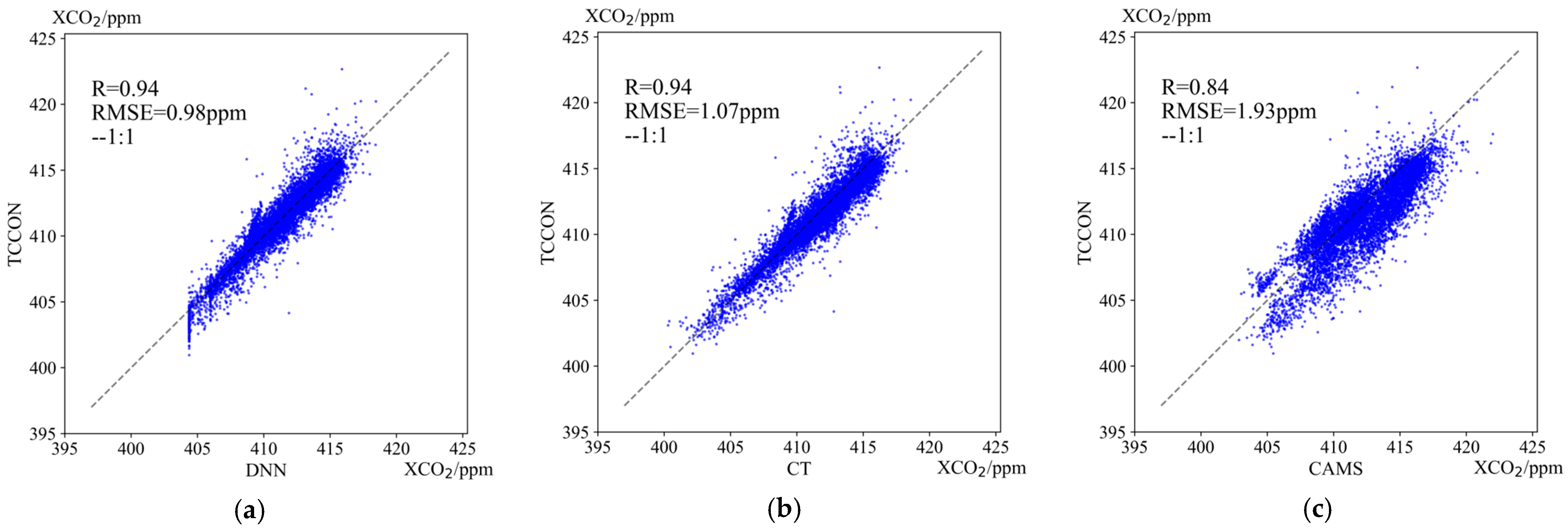
3.3. Comparison of DNN and Other Datasets
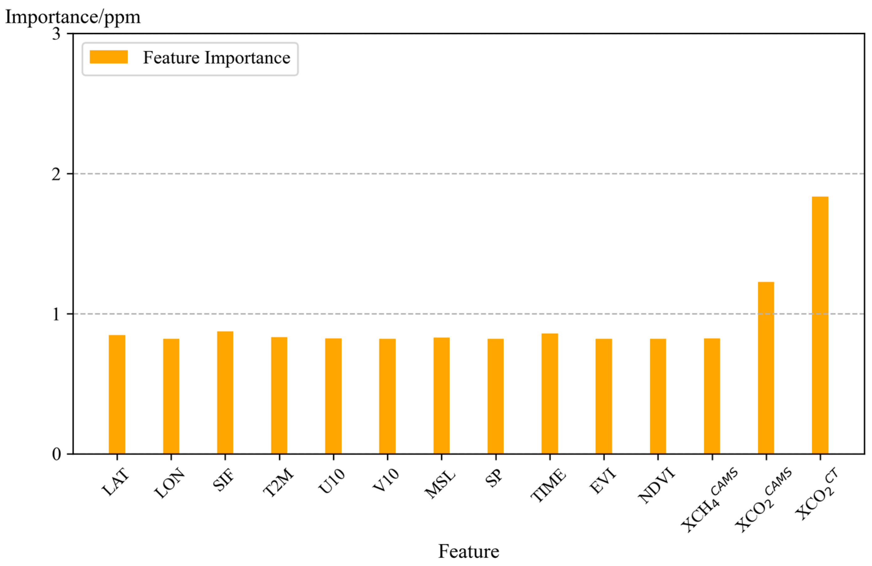
3.4. Correlation and Importance of Features
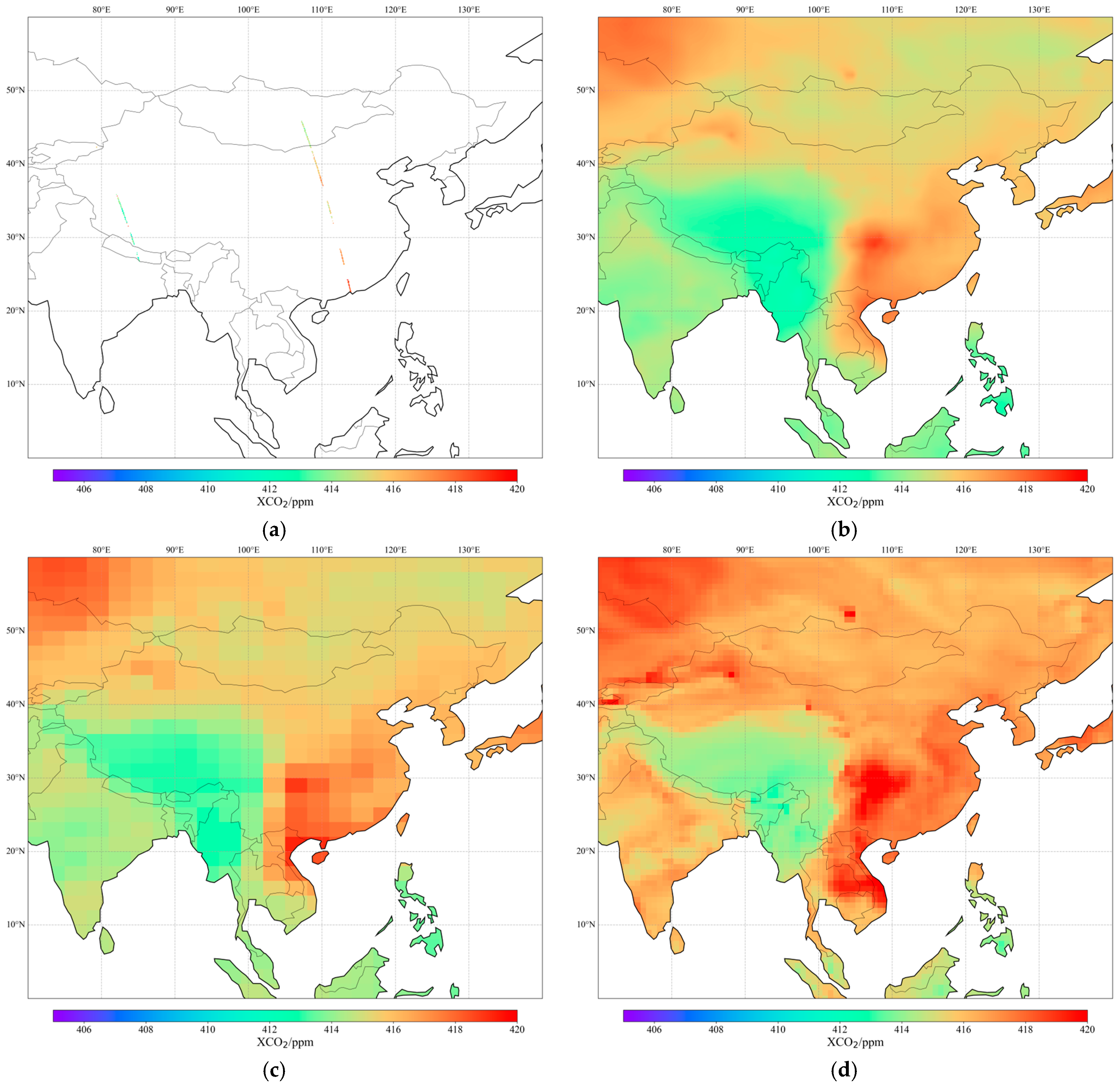
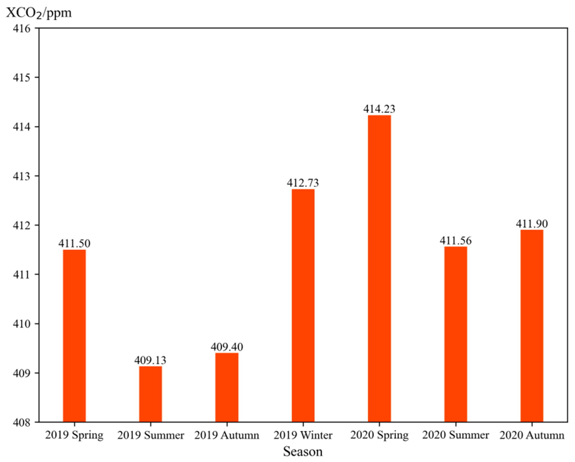
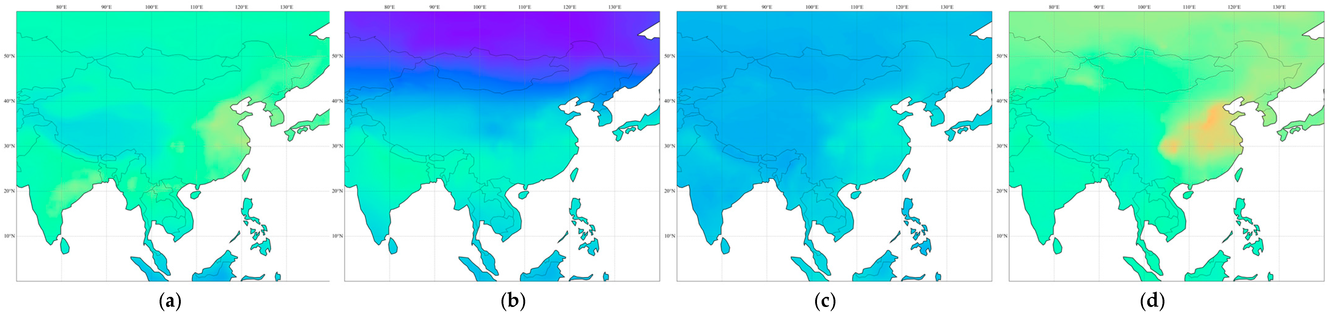
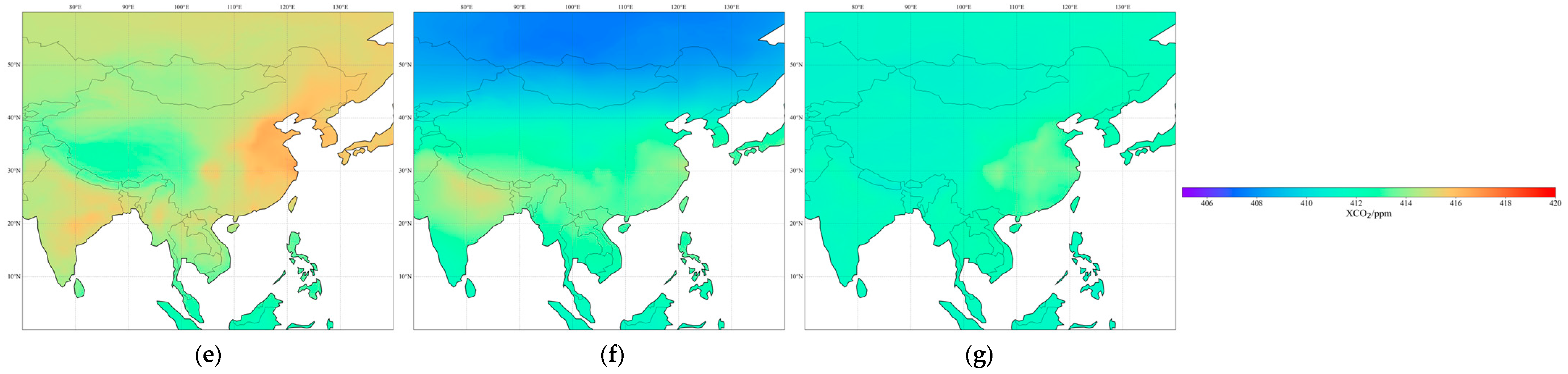
3.5. Spatial–Temporal Characteristics of China and Its Surrounding XCO2
4. Discussion
5. Conclusions
Author Contributions
Funding
Institutional Review Board Statement
Informed Consent Statement
Data Availability Statement
Conflicts of Interest
References
- Sun, Y.; Yin, H.; Wang, W.; Shan, C.; Notholt, J.; Palm, M.; Liu, K.; Chen, Z.; Liu, C. Monitoring greenhouse gases (GHGs) in China: Status and perspective. Atmos. Meas. Tech. 2022, 15, 4819–4834. [Google Scholar] [CrossRef]
- Tarasova, O.; Vermeulen, A.; Sawa, Y.; Houweling, S.; Dlugokencky, E. The State of Greenhouse Gases in the Atmosphere Using Global Observations through 2021; Copernicus Meetings: New York, NY, USA, 2023. [Google Scholar]
- Van Soest, H.L.; den Elzen, M.G.; van Vuuren, D.P. Net-zero emission targets for major emitting countries consistent with the Paris Agreement. Nat. Commun. 2021, 12, 2140. [Google Scholar] [CrossRef] [PubMed]
- Zhao, X.; Ma, X.; Chen, B.; Shang, Y.; Song, M. Challenges toward carbon neutrality in China: Strategies and countermeasures. Resour. Conserv. Recycl. 2022, 176, 105959. [Google Scholar] [CrossRef]
- Wang, Z.; Ma, P.; Zhang, L.; Chen, H.; Zhao, S.; Zhou, W.; Chen, C.; Zhang, Y.; Zhou, C.; Mao, H.; et al. Systematics of atmospheric environment monitoring in China via satellite remote sensing. Air Qual. Atmos. Health 2021, 14, 157–169. [Google Scholar] [CrossRef]
- Liangyun, L.; Liangfu, C.; Yi, L.; Dongxu, Y.; Zhang, X.; Naimeng, L.; Jiang, F.; Zengshan, Y.; Guohua, L.; Longfei, T. Satellite remote sensing for global stocktaking: Methods, progress and perspectives. Natl. Remote Sens. Bull. 2022, 26, 243–267. [Google Scholar]
- Boesch, H.; Toon, G.C.; Sen, B.; Washenfelder, R.A.; Wennberg, P.O.; Buchwitz, M.; de Beek, R.; Burrows, J.P.; Crisp, D.; Christi, M.; et al. Space-based near-infrared CO2 measurements:: Testing the Orbiting Carbon Observatory retrieval algorithm and validation concept using SCIAMACHY observations over Park Falls, Wisconsin. J. Geophys. Res. Atmos. 2006, 111, D007080. [Google Scholar] [CrossRef]
- Inoue, M.; Morino, I.; Uchino, O.; Miyamoto, Y.; Yoshida, Y.; Yokota, T.; Machida, T.; Sawa, Y.; Matsueda, H.; Sweeney, C.; et al. Validation of XCO2 derived from SWIR spectra of GOSAT TANSO-FTS with aircraft measurement data. Atmos. Chem. Phys. 2013, 13, 9771–9788. [Google Scholar] [CrossRef]
- Sun, Y.; Frankenberg, C.; Jung, M.; Joiner, J.; Guanter, L.; Kohler, P.; Magney, T. Overview of Solar-Induced chlorophyll Fluorescence (SIF) from the Orbiting Carbon Observatory-2: Retrieval, cross-mission comparison, and global monitoring for GPP. Remote Sens. Environ. 2018, 209, 808–823. [Google Scholar] [CrossRef]
- Gogoi, M.M.; Babu, S.S.; Imasu, R.; Hashimoto, M. Satellite (GOSAT-2 CAI-2) retrieval and surface (ARFINET) observations of aerosol black carbon over India. Atmos. Chem. Phys. 2023, 23, 8059–8079. [Google Scholar] [CrossRef]
- Taylor, T.E.; Eldering, A.; Merrelli, A.; Kiel, M.; Somkuti, P.; Cheng, C.; Rosenberg, R.; Fisher, B.; Crisp, D.; Basilio, R.; et al. OCO-3 early mission operations and initial (vEarly) XCO2 and SIF retrievals. Remote Sens. Environ. 2020, 251, 112032. [Google Scholar] [CrossRef]
- Du, S.; Liu, L.; Liu, X.; Zhang, X.; Zhang, X.; Bi, Y.; Zhang, L. Retrieval of global terrestrial solar-induced chlorophyll fluorescence from TanSat satellite. Sci. Bull. 2018, 63, 1502–1512. [Google Scholar] [CrossRef]
- He, Z.; Lei, L.; Zhang, Y.; Sheng, M.; Wu, C.; Li, L.; Zeng, Z.-C.; We, L.R. Spatio-Temporal Mapping of Multi-Satellite Observed Column Atmospheric CO2 Using Precision-Weighted Kriging Method. Remote Sens. 2020, 12, 576. [Google Scholar] [CrossRef]
- Johnson, M.S.; Schwandner, F.M.; Potter, C.S.; Nguyen, H.M.; Bell, E.; Nelson, R.R.; Philip, S.; O’Dell, C.W. Carbon Dioxide Emissions During the 2018 Kilauea Volcano Eruption Estimated Using OCO-2 Satellite Retrievals. Geophys. Res. Lett. 2020, 47, e2020gl090507. [Google Scholar] [CrossRef]
- Su, X.; Wang, L.; Gui, X.; Yang, L.; Li, L.; Zhang, M.; Qin, W.; Tao, M.; Wang, S.; Wang, L. Retrieval of total and fine mode aerosol optical depth by an improved MODIS Dark Target algorithm. Environ. Int. 2022, 166, 107343. [Google Scholar] [CrossRef]
- Bhattacharjee, S.; Dill, K.; Chen, J. Forecasting Interannual Space-based CO2 Concentration using Geostatistical Mapping Approach. In Proceedings of the 2020 IEEE International Conference on Electronics, Computing and Communication Technologies (CONECCT), Bangalore, India, 2–4 July 2020; pp. 1–6. [Google Scholar]
- Li, J.; Jia, K.; Wei, X.; Xia, M.; Chen, Z.; Yao, Y.; Zhang, X.; Jiang, H.; Yuan, B.; Tao, G.; et al. High-spatiotemporal resolution mapping of spatiotemporally continuous atmospheric CO2 concentrations over the global continent. Int. J. Appl. Earth Obs. Geoinf. 2022, 108, 102743. [Google Scholar] [CrossRef]
- Siabi, Z.; Falahatkar, S.; Alavi, S.J. Spatial distribution of XCO2 using OCO-2 data in growing seasons. J. Environ. Manag. 2019, 244, 110–118. [Google Scholar] [CrossRef]
- Sun, B.; Han, S.; Li, W. Effects of the polycentric spatial structures of Chinese city regions on CO2 concentrations. Transp. Res. Part D-Transp. Environ. 2020, 82, 102333. [Google Scholar] [CrossRef]
- Wei, C.; Wang, M.; Fu, Q.; Dai, C.; Huang, R.; Bao, Q. Temporal characteristics of greenhouse gases (CO2 and CH4) in the megacity Shanghai, China: Association with air pollutants and meteorological conditions. Atmos. Res. 2020, 235, 104759. [Google Scholar] [CrossRef]
- Zhang, H.; Peng, J.; Wang, R.; Zhang, J.; Yu, D. Spatial planning factors that influence CO2 emissions: A systematic literature review. Urban Clim. 2021, 36, 100809. [Google Scholar] [CrossRef]
- Zeng, J.; Nojiri, Y.; Nakaoka, S.i.; Nakajima, H.; Shirai, T. Surface ocean CO2 in 1990–2011 modelled using a feed-forward neural network. Geosci. Data J. 2015, 2, 47–51. [Google Scholar] [CrossRef]
- He, C.; Ji, M.; Li, T.; Liu, X.; Tang, D.; Zhang, S.; Luo, Y.; Grieneisen, M.L.; Zhou, Z.; Zhan, Y. Deriving Full-Coverage and Fine-Scale XCO2 Across China Based on OCO-2 Satellite Retrievals and CarbonTracker Output. Geophys. Res. Lett. 2022, 49, e2022gl098435. [Google Scholar] [CrossRef]
- Zhang, M.; Liu, G. Mapping contiguous XCO2 by machine learning and analyzing the spatio-temporal variation in China from 2003 to 2019. Sci. Total Environ. 2023, 858, 159588. [Google Scholar] [CrossRef]
- Zhang, L.; Li, T.; Wu, J. Deriving gapless CO2 concentrations using a geographically weighted neural network: China, 2014–2020. Int. J. Appl. Earth Obs. Geoinf. 2022, 114, 103063. [Google Scholar] [CrossRef]
- Jin, C.; Xue, Y.; Yuan, T.; Zhao, L.; Jiang, X.; Sun, Y.; Wu, S.; Wang, X. Retrieval anthropogenic CO2 emissions from OCO-2 and comparison with gridded emission inventories. J. Clean. Prod. 2024, 448, 141418. [Google Scholar] [CrossRef]
- Philip, S.; Johnson, M.S.; Baker, D.F.; Basu, S.; Tiwari, Y.K.; Indira, N.K.; Ramonet, M.; Poulter, B. OCO-2 Satellite-Imposed Constraints on Terrestrial Biospheric CO2 Fluxes Over South Asia. J. Geophys. Res. Atmos. 2022, 127, e2021jd035035. [Google Scholar] [CrossRef]
- Peters, W.; Jacobson, A.R.; Sweeney, C.; Andrews, A.E.; Conway, T.J.; Masarie, K.; Miller, J.B.; Bruhwiler, L.M.P.; Petron, G.; Hirsch, A.I.; et al. An atmospheric perspective on North American carbon dioxide exchange: CarbonTracker. Proc. Natl. Acad. Sci. USA 2007, 104, 18925–18930. [Google Scholar] [CrossRef]
- Chen, H.W.; Zhang, L.N.; Zhang, F.; Davis, K.J.; Lauvaux, T.; Pal, S.; Gaudet, B.; DiGangi, J.P. Evaluation of Regional CO2 Mole Fractions in the ECMWF CAMS Real-Time Atmospheric Analysis and NOAA CarbonTracker Near-Real-Time Reanalysis With Airborne Observations From ACT-America Field Campaigns. J. Geophys. Res.-Atmos. 2019, 124, 8119–8133. [Google Scholar] [CrossRef]
- Inness, A.; Ades, M.; Agusti-Panareda, A.; Barre, J.; Benedictow, A.; Blechschmidt, A.-M.; Dominguez, J.J.; Engelen, R.; Eskes, H.; Flemming, J.; et al. The CAMS reanalysis of atmospheric composition. Atmos. Chem. Phys. 2019, 19, 3515–3556. [Google Scholar] [CrossRef]
- Guevara, M.; Jorba, O.; Tena, C.; van der Gon, H.D.; Kuenen, J.; Elguindi, N.; Darras, S.; Granier, C.; Perez Garcia-Pando, C. Copernicus Atmosphere Monitoring Service TEMPOral profiles (CAMS-TEMPO): Global and European emission temporal profile maps for atmospheric chemistry modelling. Earth Syst. Sci. Data 2021, 13, 367–404. [Google Scholar] [CrossRef]
- Zhang, L.; Li, T.; Wu, J.; Yang, H. Global estimates of gap-free and fine-scale CO2 concentrations during 2014–2020 from satellite and reanalysis data. Environ. Int. 2023, 178, 108057. [Google Scholar] [CrossRef]
- Li, T.; Wu, J.; Wang, T. Generating daily high-resolution and full-coverage XCO2 across China from 2015 to 2020 based on OCO-2 and CAMS data. Sci. Total Environ. 2023, 893, 164921. [Google Scholar] [CrossRef] [PubMed]
- Malina, E.; Veihelmann, B.; Buschmann, M.; Deutscher, N.M.; Feist, D.G.; Morino, I. On the consistency of methane retrievals using the Total Carbon Column Observing Network (TCCON) and multiple spectroscopic databases. Atmos. Meas. Tech. 2022, 15, 2377–2406. [Google Scholar] [CrossRef]
- Messerschmidt, J.; Geibel, M.C.; Blumenstock, T.; Chen, H.; Deutscher, N.M.; Engel, A.; Feist, D.G.; Gerbig, C.; Gisi, M.; Hase, F.; et al. Calibration of TCCON column-averaged CO2: The first aircraft campaign over European TCCON sites. Atmos. Chem. Phys. 2011, 11, 10765–10777. [Google Scholar] [CrossRef]
- Bai, J.; Zhang, H.; Sun, R.; Li, X.; Xiao, J.; Wang, Y. Estimation of global GPP from GOME-2 and OCO-2 SIF by considering the dynamic variations of GPP-SIF relationship. Agric. For. Meteorol. 2022, 326, 109180. [Google Scholar] [CrossRef]
- Zhang, Y.; Joiner, J.; Alemohammad, S.H.; Zhou, S.; Gentine, P. A global spatially contiguous solar-induced fluorescence (CSIF) dataset using neural networks. Biogeosciences 2018, 15, 5779–5800. [Google Scholar] [CrossRef]
- Meng, L.; Liu, H.; Zhang, X.; Ren, C.; Ustin, S.; Qiu, Z.; Xu, M.; Guo, D. Assessment of the effectiveness of spatiotemporal fusion of multi-source satellite images for cotton yield estimation. Comput. Electron. Agric. 2019, 162, 44–52. [Google Scholar] [CrossRef]
- Munoz-Sabater, J.; Dutra, E.; Agusti-Panareda, A.; Albergel, C.; Arduini, G.; Balsamo, G.; Boussetta, S.; Choulga, M.; Harrigan, S.; Hersbach, H.; et al. ERA5-Land: A state-of-the-art global reanalysis dataset for land applications. Earth Syst. Sci. Data 2021, 13, 4349–4383. [Google Scholar] [CrossRef]
- Zhu, J.; Xie, A.; Qin, X.; Wang, Y.; Xu, B.; Wang, Y. An Assessment of ERA5 Reanalysis for Antarctic Near-Surface Air Temperature. Atmosphere 2021, 12, 217. [Google Scholar] [CrossRef]
- Willems, S.; Vanden Bussche, P.; Van Poel, E.; Collins, C.; Klemenc-Ketis, Z.; Pati, E.Q.E.A.Q. Moving forward after the COVID-19 pandemic: Lessons learned in primary care from the multi-country PRICOV-19 study. Eur. J. Gen. Pract. 2024, 30, 2328716. [Google Scholar] [CrossRef]
- Das, C.; Kunchala, R.K.; Chandra, N.; Chhabra, A.; Pandya, M.R. Characterizing the regional XCO2 variability and its association with ENSO over India inferred from GOSAT and OCO-2 satellite observations. Sci. Total Environ. 2023, 902, 166176. [Google Scholar] [CrossRef]
- Wu, C.; Ju, Y.; Yang, S.; Zhang, Z.; Chen, Y. Reconstructing annual XCO2 at a 1 km × 1 km spatial resolution across China from 2012 to 2019 based on a spatial CatBoost method. Environ. Res. 2023, 236, 116866. [Google Scholar] [CrossRef] [PubMed]
- Gao, P.; Yue, S.; Chen, H. Carbon emission efficiency of China’s industry sectors: From the perspective of embodied carbon emissions. J. Clean. Prod. 2021, 283, 124655. [Google Scholar] [CrossRef]
- Ge, W.; Cao, H.; Li, H.; Zhang, Q.; Wen, X.; Zhang, C.; Mativenga, P. Data-driven carbon emission accounting for manufacturing systems based on meta-carbon-emission block. J. Manuf. Syst. 2024, 74, 141–156. [Google Scholar] [CrossRef]
- Wang, W.; Hu, Y.; Lu, Y. Driving forces of China’s provincial bilateral carbon emissions and the re-definition of corresponding responsibilities. Sci. Total Environ. 2023, 857, 159404. [Google Scholar] [CrossRef]
- Zhang, C.; Song, K.; Wang, H.; Randhir, T.O. Carbon budget management in the civil aviation industry using an interactive control perspective. Int. J. Sustain. Transp. 2020, 15, 30–39. [Google Scholar] [CrossRef]
- Ji, Z.; Song, H.; Lei, L.; Sheng, M.; Guo, K.; Zhang, S. A Novel Approach for Predicting Anthropogenic CO2 Emissions Using Machine Learning Based on Clustering of the CO2 Concentration. Atmosphere 2024, 15, 323. [Google Scholar] [CrossRef]
- Zhang, Y.; Liu, X.; Lei, L.; Liu, L. Estimating Global Anthropogenic CO2 Gridded Emissions Using a Data-Driven Stacked Random Forest Regression Model. Remote Sens. 2022, 14, 3899. [Google Scholar] [CrossRef]


| Time | 2019 | 2020 | |
|---|---|---|---|
| FH | 1 January–30 June | 170 × 105 | 161 × 105 |
| SH | 1 July–31 December | 169 × 105 | 164 × 105 |
| Use Model | Train Time | Unknown Time |
|---|---|---|
| 19FH | 1 January 2019–30 June 2019 | 1 July 2019–10 July 2019 |
| 19SH | 1 July 2019–31 December 2019 | 20 June 2019–30 June 2019 1 January 2020–10 January 2020 |
| 20FH | 1 January 2020–30 June 2020 | 21 December 2019–31 December 2019 1 July 2020–10 July 2020 |
| 20SH | 1 July 2020–31 December 2020 | 20 June 2020–30 June 2020 |
Disclaimer/Publisher’s Note: The statements, opinions and data contained in all publications are solely those of the individual author(s) and contributor(s) and not of MDPI and/or the editor(s). MDPI and/or the editor(s) disclaim responsibility for any injury to people or property resulting from any ideas, methods, instructions or products referred to in the content. |
© 2024 by the authors. Licensee MDPI, Basel, Switzerland. This article is an open access article distributed under the terms and conditions of the Creative Commons Attribution (CC BY) license (https://creativecommons.org/licenses/by/4.0/).
Share and Cite
Tian, W.; Zhang, L.; Yu, T.; Yao, D.; Zhang, W.; Wang, C. Generating Daily High-Resolution Regional XCO2 by Deep Neural Network and Multi-Source Data. Atmosphere 2024, 15, 985. https://doi.org/10.3390/atmos15080985
Tian W, Zhang L, Yu T, Yao D, Zhang W, Wang C. Generating Daily High-Resolution Regional XCO2 by Deep Neural Network and Multi-Source Data. Atmosphere. 2024; 15(8):985. https://doi.org/10.3390/atmos15080985
Chicago/Turabian StyleTian, Wenjie, Lili Zhang, Tao Yu, Dong Yao, Wenhao Zhang, and Chunmei Wang. 2024. "Generating Daily High-Resolution Regional XCO2 by Deep Neural Network and Multi-Source Data" Atmosphere 15, no. 8: 985. https://doi.org/10.3390/atmos15080985