Abstract
The analysis of rainfall patterns in the Indonesian region utilized the Empirical Orthogonal Function (EOF) method to identify spatial and temporal variations. The study evaluated the dynamic influence of the Tropical Indian Ocean (TIO) and the Tropical Pacific Ocean (TPO) on Indonesian rainfall using monthly data from the Southeast Asian Climate Assessment and Dataset (SACA&D) spanning from January 1981 to December 2016 and encompassing three extreme El Niño events in 1982/1983, 1997/1998 and 2015/2016. Using combined reanalysis and gridded-observation data, this study evaluates the potential impact of the two primary modes in the tropical Indo-Pacific region, namely the Indian Ocean Dipole (IOD) and the El Niño-Southern Oscillation (ENSO) on Indonesian rainfall. The analysis using the EOF method revealed two main modes with variances of 35.23% and 13.07%, respectively. Moreover, the results indicated that rainfall in Indonesia is highly sensitive to sea surface temperatures (SST) in the southeastern tropical Indian Ocean and the central Pacific Ocean (Niño3.4 and Niño3 areas), suggesting that changes in SST could significantly alter rainfall patterns in the region. This research is useful for informing government policies related to anticipating changes in rainfall variability as part of Indonesia’s preparedness for hydrometeorological disasters.
1. Introduction
One of the direct factors that influences differences in climate type or variation is rainfall [1]. The most important factor that influences the intensity of rainfall received by an area is topography. Indonesia’s unique topography triggers differences in the intensity of rainfall received according to the local character of each region. High rainfall has the potential to cause flooding and landslides. Conversely, low rainfall intensity can trigger long droughts, which are the main factors causing haze disasters [2]. In 2015, based on recapitulation data of disaster events and impacts from the National Disaster Management Agency in Indonesia, there were 2342 disaster events in Indonesia. Peatland fires, floods, landslides, and tornadoes accounted for 92% of these hydrometeorological disasters. The main cause of floods and landslides is none other than high rainfall, while land and peat fires are caused by the long dry season, resulting in haze that impacts wildlife, human health, the economy, and climate [3]. More than 100–300 people died in Indonesia, Malaysia, and Singapore due to poor air quality, which was most likely caused by the spread of haze during September–October 2015 [4]. Based on these data, rainfall is a very important climate parameter in determining the dynamics of climate change, which has a significant impact on the availability of water resources. Therefore, a comprehensive and in-depth understanding of the precise character of rainfall pattern variations needs to be carried out as a form of disaster preparedness, anticipation, and commitment to the proper and comprehensive management of water energy sources.
Rainfall in the Indonesian region is generally influenced by several phenomena, including the diurnal cycle [5], the Madden Julian Oscillation (MJO) [6], Asia–Australia Monsoon [7], El Niño Southern Oscillation (ENSO) [8,9,10,11] and Indian Ocean Dipole (IOD) [12,13]. Rainfall variability in Indonesia is complex and part of monsoon variability [7]. The study focuses on identifying and analyzing the signals of the Indonesian monsoon using Space–Time Singular Value Decomposition (SVD). The temporal evolution of these modes is linked with significant climatic events, providing insights into monsoon predictability [14,15,16]. The monsoon [17,18] and the movement of the Inter-Tropical Convergence Zone (ITCZ) [7,19] are related to annual and semi-annual rainfall variations in Indonesia, while the El Niño and Dipole Mode phenomena are related to interannual rainfall variations in Indonesia [9,10,13,20,21]. It was known that El Niño and positive IOD events cause rainfall deficits in the Indonesian region [1,2,22,23].
Understanding climate variability is essential for actual projections of future climate change. Not many studies have revealed the impact of changes in Indo-Pacific climate modes on rainfall variability. The main issue addressed in this study is the spatial and temporal pattern of rainfall in Indonesia and its relation to the tropical Indo-Pacific climate mode. Previous studies have investigated the correlation of changes in Indo-Pacific tropical mean conditions due to global warming with the properties of climate modes [14]. Increasing sea surface temperature (SST) and internal variability are the main sources of uncertainty in determining modal changes. Internal climate variability remains a major challenge in predicting changes in climate modes. An Indo-Pacific phenomenon that has received much attention is the El Niño Southern Oscillation (ENSO), which occurs every three to seven years and affects the Earth’s weather during the year [24,25]. Under normal circumstances, the sea surface temperature of the western Pacific Ocean is warmer (the warm pool) than the eastern part. When El Niña occurs, the warm pool shifts to the east so that the eastern Pacific SST becomes warmer and the shallow eastern Pacific thermocline layer becomes deeper [26,27]. El Niño causes the western equatorial part of the Americas to experience heavy rains that can cause flooding, and conversely, Indonesia and other tropical regions directly adjacent to the Pacific Ocean equator will experience drought [28,29]. The opposite of the EI-Niño phenomenon is La Niña. A phenomenon similar to ENSO also occurs in the Indian Ocean, called the Indian Ocean Dipole (IOD). This IOD certainly causes extreme weather changes in tropical areas directly adjacent to the Indian Ocean, including Indonesia [12,20].
Previous research has described three distinct rainfall areas in Indonesia: monsoonal, equatorial, and local [7]. The monsoonal region covers southern and central parts of Indonesia, from South Sumatra to Timor Island, parts of Kalimantan, parts of Sulawesi, and parts of Irian Jaya [17,18]. The equatorial region is located in northwestern Indonesia and covers the northern part of Sumatra and the northwestern part of Kalimantan. The local region includes Maluku and parts of Sulawesi (close to the western Pacific region). The monsoonal pattern is influenced by the monsoon system, which is characterized by the movement from high pressure to low pressure over the continents of Asia and Australia alternately [17,24]. The semi-monsoonal pattern is an equatorial pattern or a pattern of two peaks of maximum rainfall associated with the movement of the ITCZ [7,21], which passes the equator twice a year, forming a six-month cycle (semi-annual) that is simultaneously processed in the monsoon system, so it is referred to as a semi-monsoon, which occurs in the March–May (MAM) and September–November (SON) periods [28]. While the local pattern is a rainfall distribution pattern that is opposite to the monsoonal pattern, in the JJA period, the local pattern reaches maximum rainfall [7]. Annual and inter-annual climate variability in Indonesia is unique because it is not the same for all regions and affects weather and rainfall patterns [18,30].
It should be noted that the spatial and temporal variability of rainfall is strongly influenced by geographical location (location relative to oceans and continents), topography, altitude, wind direction, and latitude. Therefore, mapping rainfall areas is very important to find the characteristics of rainfall that occur in each region, both spatial and temporal. However, there is a gap in scientific studies regarding the deep and comprehensive understanding of the relationship between climate modes in the Indo-Pacific region and rainfall variations in Indonesia. Understanding and knowledge of climate characteristics and dynamics in each region is an important aspect of better mitigation efforts, especially in preventing and determining the right preventive attitude towards the negative impacts of hydrometeorological disasters. The topography of Indonesia, which is surrounded by oceans and located between two continents, determines the character of the rainfall cycle. Therefore, this study aims to analyze and identify the characteristics of rainfall in Indonesia and relate them to the dynamics of climate phenomena in the Indo-Pacific Region as a whole. This study evaluates and observes phenomena along the equator of the Indian Ocean and Pacific Ocean, namely the Tropical Indian Ocean (TIO) and Tropical Pacific Ocean (TPO), to illustrate how much influence they have on rainfall patterns in Indonesia. The results of this research are expected to be able to clearly and precisely describe rainfall patterns in Indonesia to prepare a preventive attitude in facing the threat of hydrometeorological disasters that are very vulnerable to occurring in the territory of Indonesia.
2. Materials and Methods
2.1. Study Location
Indonesia is an archipelagic country that has a complex topography, as shown in Figure 1. The height of land in Indonesia varies between 0 and 4884 m above sea level [22]. Geologically, the presence of land that forms large islands in this region has an influence on the process of mass and heat transport between the Indian and Pacific Oceans [23]. This land also supports the process of transferring heat from the sea to the atmosphere, thereby increasing rainfall in this area. Apart from that, the interaction between land and wind also has an important influence on variations in rainfall intensity in this region [10,31,32].
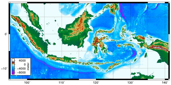
Figure 1.
Topography of Indonesian region. Source: https://tanahair.indonesia.go.id (accessed on 5 January 2023).
2.2. Data Collection
Monthly rainfall data covering the period January 1981 to December 2016 with a horizontal resolution of 0.25° × 0.25° are taken from the Southeast Asian Climate Assessment and Dataset (SACA&D) data at the link http://sacad.bmkg.go.id/download/grid/download.php (accessed on 8 November 2022). This dataset was developed by the study area of Southeast Asia (SA-OBS) whose validity has been tested, a high-resolution daily gridded dataset of surface temperature and precipitation specifically designed for Southeast Asia [33]. The dataset was created to address the need for accurate and consistent climate data to support research, climate monitoring, and modeling efforts in the region. In addition to rainfall data, this study also used monthly Sea Surface Temperature (SST) data from ERA5 monthly averaged data at the link https://cds.climate.copernicus.eu/ (accessed on 2 January 2023), Dipole Mode Index (DMI) from Japan Agency for Marine-Earth Science and Technology (JAMSTEC), Niño3.4 Index, Vertical Velocity, zonal wind (u10), and meridional (v10) published by NCEP/NCAR at the link https://psl.noaa.gov/data/gridded/data.ncep.reanalysis.html (accessed on 2 March 2023). ERA5 provides climate data with very high spatial and temporal resolution, enabling detailed and accurate analysis of climate and weather variations. This is very useful for regional as well as global studies. Data from ERA5 is the result of combining observational data and models, which provides more accurate results than using only observational data or models.
2.3. Data Analysis
The method used in this research was the empirical orthogonal function (EOF) analysis method. EOF was a method for determining dominant patterns determined by data and evolving in space and time [34]. The main objective of EOF analysis was to reduce a large number of data variables to only a few variables without changing most of the variance of the original data [35,36]. The EOF method could identify spatial and temporal patterns of rainfall in the Indonesian region and classify the spatial and temporal patterns recorded in the data. The first analysis of rainfall was performed monthly on rainfall at 60 stations in Nevada [28]. Meanwhile, the identification of rainfall in Indonesia using EOF has been classified as monsoon, equatorial, and local [7]. In this study, EOF analysis was conducted on SACA&D monthly rainfall for 35 years for the period January 1981–December 2016. The procedure for computing eigenvectors from a matrix of data has been described extensively in the literature [37,38].
Let represent a set of observation vectors at each rainfall data for observations in time of variables. The EOF analysis was started by determining the covariance matrix of the rainfall data matrix that has been arranged, namely
where represents an eigenvector associated with the ith eigenvalue and is the time-dependent coefficient of the ith eigenvector for the nth observation in time [29]. In this case, the total number N of observations is equal to 420 (35 years of monthly rainfall data). The Theoretical–Methodological Flowchart for this research is shown in Figure 2
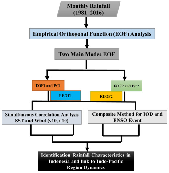
Figure 2.
Theoretical–Methodological Flowchart.
The EOF technique was used to examine the spatial and temporal variations of all parameters (rainfall data). EOF analysis extracts multivariate datasets into a series of orthogonal functions or modes based on the covariance matrix of the data [29,30]. Every mode consists of the spatial eigenfunctions, representing the spatial patterns of variability at each time and the principal components, where a time series shows how the spatial pattern varied with time. Each subsequent mode was orthogonal, which is consistently the same as the previous one. Typically, the leading mode explains the highest amount of the total variance in which the variations of its spatial and temporal patterns are strongly coupled [10]. It should be noted that the EOF approach is restricted by several criteria, such as the requirement for orthogonal spatial modes and the dependency of the solution on the region of study [28,39].
Testing the relationship of rainfall to ENSO and IOD was conducted by observing the impact of both climate modes on rainfall across Indonesia. The dynamics of the influence of IOD and ENSO on rainfall in the Indonesian region were evaluated using composite techniques [30,31]. The composite analysis is applied to each climate mode event, namely IOD positive, IOD negative, El Niño, and La Niña. Composite analysis involves collecting a large number of cases of observed climate phenomena. Composite analysis is performed to assess the variability of parameters at time t from rainfall, SST, and wind data [10,32]. Dipole Mode Index (DMI) and Niño3.4 index were used to classify IOD and ENSO events. The intensity of IOD is represented by the SST gradient, which is an anomaly between the western equatorial Indian Ocean (50° E–70° BT and 10° S–10° N) and the southeastern equatorial Indian Ocean (90° BT–110° BT and 10° S–10° N) [20] and is referred to as the Dipole Mode Index (DMI). The DMI index is the basis for the classification of positive (negative) IOD. The DMI index is the basis for the classification of positive (negative) IOD. El Niño (La Niña) events occur when the average standard deviation is >1 (<−1) for five consecutive months. Meanwhile, the positive (negative) IOD event is identified when the average standard deviation is >1 (<−1) for 3 consecutive months [30]. Neutral years without IOD and ENSO phenomena are also observed by researchers by looking at the average SST in these neutral years. This is to see the dynamics of SST and wind when no IOD or ENSO phenomena occur. SST anomalies to determine the Indo-Pacific climate mode phenomenon are shown in Figure 3.
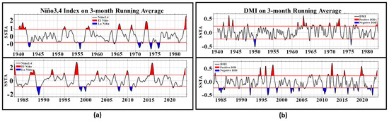
Figure 3.
Time series of (a) Niño3.4 index and (b) Dipole Mode Index from 1940–2020.
Researchers classify ENSO and IOD phenomena in the Pacific Ocean and the Indian Ocean by referring to the calculation of Niño3.4 values for five consecutive months and DMI for three consecutive months. It should be noted that the seasonal period taken in this study is the end of the dry season, August–September–October (ASO) and the beginning of the rainy season, November–December–January (NDJ). The peak of ENSO occurs at the end of the dry season, namely the ASO period and the peak of IOD occurs at the beginning of the rainy season, namely the NDJ period [18,19]. The classification results obtained are 8 El Niño, 3 La Niña, and 14 neutral years for the ENSO phase, while 10 positive IOD and 9 negative IOD are for the IOD phase (Table 1).

Table 1.
Classification of El Niño/La Niña and positive/negative IOD years and neutral years (non-El Niño/La Niña and/or non-positive/negative IOD).
3. Results
3.1. Spatial and Temporal Patterns of Rainfall in Indonesia
We considered the two main modes of EOF because, based on the results of the variance produced, it has met the minimum requirement for analysis, which is 51.30%, and describes the dominant climate variability in Indonesia as a whole. The spatial patterns PC1 and PC2 from the EOF method are complemented by the time series coefficients of each spatial PC (EOF1 and EOF2) shown in Figure 4a,b. PC1 and PC2 explain 38.23% and 13.07% of all variances, respectively, and have explained more than half of the total variance of the entire dataset over 35 years or 420 months.
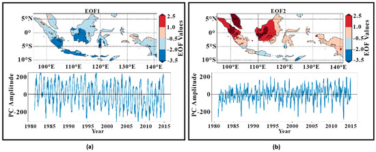
Figure 4.
Spatial patterns of eigenfunctions (upper panel) and time series of principal component (lower panel) of (a) EOF mode 1; (b) EOF mode 2.
The identification results in EOF1 are based on regional division covering most of southern Indonesia and the most dominant variability in the entire dataset. In EOF1, it could be seen that homogeneous areas show negative anomaly patterns, but the strongest negative anomalies appear in southern Sumatra, Java, southern Kalimantan, southern Sulawesi, and other islands in southern Indonesia. Only a few areas show positive anomalies, namely northern Sumatra, the Maluku Islands, and northern Papua. However, EOF2 reveals that rainfall variability in the western part of Indonesia differed from that in its eastern part. EOF2 was dominated by positive anomalies, but they are strongest in northern Sumatra and western to northern Kalimantan. EOF2 also shows some areas with negative anomalies, namely in southern Sumatra, southern Java, Bali Island, southern Sulawesi, NTB, NTT, and a small part of southern Papua Island.
The climatology of each region shows that each region has its own characteristics. The EOF1 region has one peak and one trough, while the EOF2 region has two peaks: in October–November (ON) and in March–May (MAM). The climatology of the main PC shows the alignment of the results of previous studies, as shown in Figure 5.
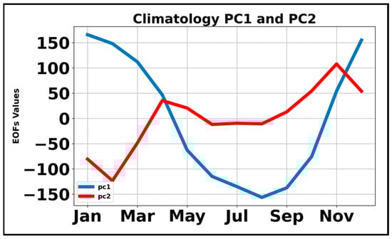
Figure 5.
Climatological time series of principal components of the first mode (blue) and the second mode (red).
Based on the results of the time series pattern spectrum in Figure 6, it was found that the EOF1 spectrum is dominated by the 12-monthly (annual) cycle. The EOF1 spectrum has a strong annual signal. This signal dominates the overall variability with a value three times the other maximums. The strong annual signal of the EOF1 region shows a strong homogeneous pattern, as also indicated by the small standard deviation of its annual cycle. Meanwhile, the spectrum of EOF2 shows that 6-monthly (semi-annual) oscillations are more dominant than annual oscillations. PC2 spectrum also shows oscillations in the intra-seasonal (<6-monthly), namely in the 4-month period. The intra-seasonal signals could be connected to variations in events that take place in the eastern tropical Indian Ocean and in the western tropical Pacific Ocean, namely the Madden Julian Oscillation (MJO) [17,18,19]. Meanwhile, the interannual signals (>12 monthly) occur with smaller amplitudes than other signals, such as 20-monthly, 105-monthly, 210-monthly, and 420-monthly signals. Therefore, the spectra of the EOF1 and EOF2 regions reveal the presence of strong ENSO and IOD-related signals. The eigenvalue spectrum of EOF1 shows the dominance of monsoon (annual) climate signal types, while EOF2 is related to equatorial (semi-annual) signals [7].

Figure 6.
Spectra of the time series of principal component of (a) the first mode and (b) the second mode.
The distribution of spatial and temporal variations of rainfall was reconstructed to reorganize the data and confirm the correctness of the previously obtained EOF results. The reconstructed EOF1 is called REOF1, and EOF2 is called REOF2. This is performed to identify the spatial pattern of rainfall variation in the Indonesian region as a whole. The spatial mean and spatial standard deviation of rainfall in REOF1 and REOF2 can be seen in Figure 7a–d.
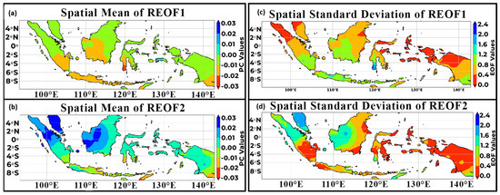
Figure 7.
Spatial mean (left panel) and spatial standard deviation (right panel) of reconstructed time series of the eigen-function of (a,c) the first mode, and (b,d) the second mode.
Based on the results of the spatial mean and standard deviations in Figure 6, the differences between regions are clear and illustrated as a whole. In REOF1, it can be seen that the average rainfall is dominant in southern Indonesia, with a large standard deviation value in the region. Meanwhile, REOF2 shows that the average rainfall is dominant in northern Sumatra and parts of Kalimantan (the western part), and it can also be seen in the standard deviation of REOF2 that there is high variability in this region. This indicates that the region with dominant rainfall has high rainfall variability, and the EOF method can capture the dominant signal in this region. What is interesting in the reconstruction results is that for the REOF2 region, Sumatra Island and Kalimantan Island, in particular, are different from the variability of other islands. The equatorial region has a different climate type from other regions. Thus, in the REOF2 region, these two islands have very large variations, and the differences between regions are very clear between the north, center, and south. However, researchers need to emphasize that the REOF1 region is the largest and dominant region based on the observations.
Monthly climatology and average monthly rainfall calculated from January 1981 to December 2016 in REOF1 and REOF2 are described in Figure 7 and Figure 8. Fluctuations in the positive phase and negative phase of the REOF1 region occur at the end of the year and the beginning of the year. The positive phase occurs at the end and beginning of the year, while the negative phase occurs from May to October. These results indicate the strong influence of two monsoons, namely the northwest monsoon associated with wet conditions and the southeast monsoon associated with dry conditions. The positive phase and negative phase fluctuations of the REOF2 region occur twice a year, namely in June–July–August (JJA) and in January–February–March (JFM) for the negative phase, while April–May (AM) and September–December (SOND) for the positive phase. The positive and negative phases of REOF2 are related to the southern and northern movements of the inter-tropical convergence zone (ITCZ) discussed earlier. The monthly spatial climatology results of REOF1 and REOF2 are consistent with the climatology of PC1 and PC2 discussed in Figure 9.
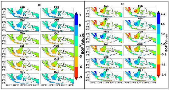
Figure 8.
Climatological mean of reconstructed time series of the eigenfunction of (a) the first mode and (b) the second mode.

Figure 9.
Monthly average of reconstructed time series of the eigenfunction of (a) the first mode and (b) the second mode. Red bars indicate decreasing in rainfall, blue bars indicate increasing in rainfall.
3.2. Relationship between Temporal Variation of Rainfall and Indo-Pacific Climate Modes
Simultaneous correlations between seasonal rainfall (ASO and NDJ) and Indo-Pacific climate modes were calculated to assess the possible influence of IOD and ENSO events on rainfall in Indonesia. Figure 10 and Figure 11 show the simultaneous correlation between PC1 and PC2 to SST and wind in the TPO and TIO regions for each season. In Figure 10a, there is a strong positive correlation between PC1 and SST of local waters around Indonesia (especially around the equatorial southeast side of the Indian Ocean) and a strong negative correlation with SST of the central Pacific Ocean (Niño3 and Niño3.4 regions). The wind correlation results show anomalously strong winds blowing from the southeast towards the equatorial center of the Indian Ocean and from eastern Indonesia towards the central Pacific Ocean, suggesting that there is a strong contrast in pressure between the two regions during the ASO season. The correlation of PC1, wind, and SST that has been described is similar to the pattern during ENSO and IOD. Thus, it can be concluded that the PC1 pattern is similar to the ENSO and IOD patterns. However, this correlation weakens during the NDJ season, as shown in Figure 10b.
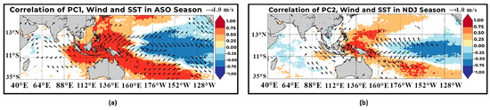
Figure 10.
Correlation between PC1 and SST for the (a) ASO season and (b) NDJ season. Red color shows positive correlation, blue color shows negative correlation. Only significant level values that are at or above the 95% level are colored. The orientation of the arrow indicates the direction of the wind, and their length is proportional to the magnitude of the correlation.
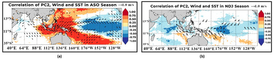
Figure 11.
Correlation between PC2 and SST for the (a) ASO season and (b) NDJ season. Only significant level values that are at or above the 95% level are colored. The orientation of the arrow indicates the direction of the wind, and their length is proportional to the magnitude of the correlation.
Figure 11 shows similarities with Figure 10, which shows the correlation between PC2, wind, and SST. In Figure 11a, showing the correlation of PC2 to winds and SST during the ASO season, the correlation results show a strong positive correlation between the dominant rainfall pattern of PC2 and local Indonesian waters and a strong negative correlation to the central Pacific Ocean. However, the correlation of PC2 is slightly weaker than that of PC1. During the NDJ season, the correlation between PC2, local SST, and the central Pacific Ocean disappears and is not correlated at all. In general, the correlation between PC2, SST, and wind is similar to that between PC1. However, it is slightly weaker. Therefore, it can be concluded that the rainfall patterns in PC1 and PC2 are similar to IOD events.
The positive correlations in Figure 10 and Figure 11 indicate that the greater the increase in local SST, the more rainfall in the Indonesian region. Significant positive correlations exist east of Australia and in some parts of the northwest Pacific Ocean. Negative correlations exist for the warm pool area (Niño3), northeastern Indonesia, and the South Pacific convergence zone. The negative correlation suggests that an increase in SST in the warm pool area triggers a decrease in rainfall over Indonesia. In general, the EOF1 region experiences a positive local SST influence but also a strong negative influence from SST and winds in the equatorial western Pacific Ocean during the ASO season. However, during the NDJ season, these influences are weakened. The response of ENSO and IOD phenomena is significant during the late dry season in Indonesia.
Thus, the EOF1 region is more strongly influenced by SST and wind along the equatorial TIO and TPO during the ASO season than the EOF2 region. Despite the different rainfall cycles in these two modes, the responses to SST and wind in the EOF1 and EOF2 regions are similar. This is in line with the results of research by Hamada (2003), which states that during the dry season in Indonesia, ocean currents will be carried by the wind moving away from Indonesian waters so that the sea level of the Indonesian maritime continent decreases, which results in low evaporation in the atmosphere and has an impact on reducing rainfall in Indonesia.
Previous observations have found a decreasing trend in the amount of accumulated monthly and annual rainfall from 1955 to 2005 in the Brantas region, East Java [19]. Additionally, they noted a reduced dominance of the monsoon, resulting in changes in annual climate patterns and an increase in the dry season [9,19]. The impact of SST and rainfall variations in the eastern equatorial waters of the Indian Ocean and Indonesian waters on the amplitude of El Niño has been investigated using modeling studies [33]. The results of this research reveal that rainfall in the eastern Indian Ocean region experienced a significant increase as El Niño developed. Furthermore, correlations were calculated between PC1 and PC2 and the Niño3.4 Index and DMI. The correlation results can be observed in Table 2.
Table 2.
Correlation between PC1 and PC2 with Niño3.4 Index and DMI.
Based on the correlation results in Table 2, it can be seen that PC1 and PC2 have a moderate negative correlation with Niño3.4 and DMI at −0.55 and −0.33, respectively. Both PC1 and PC2 are categorized as weakly to moderately correlated to DMI and the Niño3.4 index. However, PC1 is more highly correlated with ENSO and IOD. These correlation values show a moderate negative correlation [32], where if the Niño3.4 index value is positive (El Niño), there will be a decrease in rainfall during the ASO period. If there is an increase in sea surface temperature above normal in the eastern part of the Pacific Ocean, it will cause winds to move from west to east so that convection will occur quite strongly in the eastern Pacific Ocean, resulting in a decrease in the amount of rainfall in Indonesia. Likewise, the correlation of PC1 and PC2 to DMI. The negative correlation shows that when there is a positive IOD, the sea surface temperature is warmer than normal in the Western Indian Ocean, while in the East, it is cooler than normal [20], where this condition causes the wind to move from east to west so that the Indonesian region experiences a decrease in rainfall [35].
The influence of ENSO and IOD on Indonesia’s dominant rainfall patterns is further analyzed by calculating normalized anomalies in the two main mode regions. This aims to see how much influence ENSO and IOD have on the increase and decrease of rainfall in Indonesia. As expected, low EOF values were observed during the ASO season, especially in the REOF1 region, which has a very significant difference during the wet and dry seasons in this region. The normalized PC1 and PC2 anomaly results for ASO and NDJ in Figure 12 and Figure 13 show that these results are in line with the classification of El Niño/La Niña and/or positive/negative IOD years in the previous discussion. The difference in rainfall intensity is clearly illustrated by the decrease or increase in rainfall in each region. Fluctuations in the positive and negative phases are particularly evident when El Niño and IOD, as well as NIOD and La Niña, occur simultaneously.
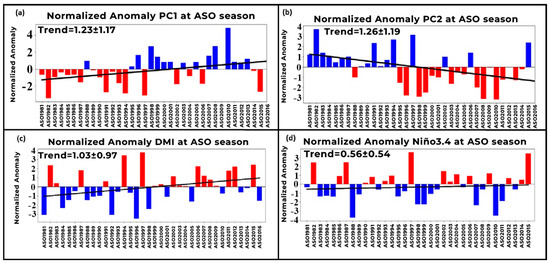
Figure 12.
Normalized anomalies at ASO season for (a) PC1, (b) PC2, (c) DMI, (d) Niño3.4 time series. Blue bars indicate positive anomalies, red bars indicate negative anomalies.
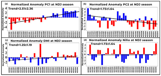
Figure 13.
Normalized anomalies at NDJ season for (a) PC1, (b) PC2, (c) DMI, (d) Niño3.4 time series. Blue bars indicate positive anomalies, red bars indicate negative anomalies.
3.3. Composite Analysis of Dominant Patterns of Rainfall in Indonesia
The influence of each climate mode event on rainfall in the Indonesian region was calculated using the composite method during IOD and El Niño/La Niña events in the ASO season and NDJ season. As a result, the ASO season forms an interconnected pattern between rainfall and climate mode indices. By referring to the classification data in Table 1, it was found that four positive IOD events coincided with El Niño events, while three negative IOD events occurred in four La Niña years and seventeen non-El Niño/La Niña years. This is influenced by the winter monsoon in the northern hemisphere and the strength of the cold and dry northern wave [7]. Figure 14 shows the average rainfall in the two main EOF mode regions in neutral years. The composite results show that the reduction of rainfall during the ASO season is depicted in the REOF1 region. During the ASO dry season, the REOF1 region tends to be in the negative phase, whereas during the NDJ season, it is in the positive phase. However, this is not seen in the REOF2 region, which has a rainfall pattern that tends to be wet throughout the season because it is in a positive phase.

Figure 14.
Composite maps of REOF1 and REOF2 anomalies during ASO (left) and NDJ (right) seasons in neutral years. REOF anomalies that are significant at the 95% level of the two-tailed t-test are marked with shaded areas.
Dry years in Indonesia with normalized anomalies ≤−1.0 occur during El Niño years such as 1982, 1986, 1991, 1994, 1997, 2002, 2006, 2009, and 2015. Three of the nine drought years were associated with positive IOD years. In contrast, wet years when normalized anomalies ≥ 1.0 occurred in 1983, 1988, 1995, 1998, 2000, 2005, 2007, 2010, and 2011. Two of the nine wet years coincided with negative IOD events (including years with concurrent La Niña events). When El Niño and positive IOD events occur, sea level decreases, and sea surface temperatures tend to be cooler during the ASO season so that zonal and meridional winds from western Indonesia move towards the western Indian Ocean [19]. This causes a reduction in evaporation activity in the atmosphere so that the water vapor formed in the clouds is lower. Finally, rainfall in Indonesia is getting lower, and long droughts and even droughts occur almost throughout the year [30,36].
Figure 15 and Figure 16 show the composite reconstruction of EOF1 (REOF1) and EOF2 (REOF2) in ASO and NDJ seasons during El Niño/La Niña and IOD (PIOD/NIOD) phenomena. During positive IOD and El Niño events, most parts of Indonesia experience rainfall deficits during the ASO season, as indicated by the dominant negative phase in both REOF1 and REOF2, but during the NDJ season, the impact of ENSO and IOD on these two regions has weakened, and the distribution of positive phases dominates throughout the region. The onset of peak rainfall occurs during the NDJ season, with southern Sumatra, Java, and southern Kalimantan receiving more rain than other regions. However, it is interesting to note that northern parts of Sumatra do not have rainfall deficits during El Niño years in the ASO season, instead tending to receive rainfall surpluses in El Niño years. This is especially true in REOF1 in the northern parts of Sumatra, Kalimantan, Sulawesi, and Papua.

Figure 15.
Composite maps of REOF1 and REOF2 anomalies during (a) El Niño and (b) La Niña. REOF anomalies that are significant at the 95% level of the two-tailed t-test are marked with shaded areas.
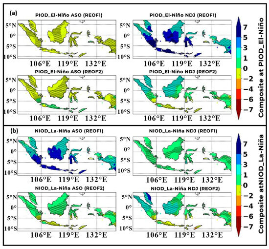
Figure 16.
Composite maps of REOF1 and REOF2 anomalies during (a) positive IOD and (b) negative IOD. REOF anomalies that are significant at the 95% level from a two-tailed t-test are marked with shaded areas.
At the end of the dry season (ASO), most parts of Indonesia covered by the REOF1 and REOF2 regions experience rainfall deficits, which are worst during concurrent El Niño and Positive IOD events, although the REOF2 region is not more severe than the REOF1 region. The rainfall composite during El Niño events shows a similar pattern to positive IOD events. However, droughts during El Niño events in the ASO season cover a larger area but are not more severe than during concurrent positive IOD events. In contrast, during La Niña events, almost all of Indonesia experiences a surplus of rainfall in the ASO season.
4. Discussion
The decrease in rainfall in the lowlands is not visible during the NDJ season but tends to increase in the Bukit Barisan area along the coastline of Sumatra Island [18]. Indonesia has been classified into five climatic regions by analyzing the amplitude and phase of annual oscillations of mean rainfall. The characteristics of these five regions are similar to the EOF1 and EOF2 regions generated in this study. However, they have not revealed the influence of the Indo-Pacific Ocean and atmospheric dynamics on rainfall regions in detail and depth. The result of The EOF analysis indicates that the variability in Sumatra and Kalimantan is significantly different from other regions, especially the northern and southern regions of these two islands. Local differences in dominant rainfall patterns for each EOF region are observed at the beginning of the rainy season during El Niño years. The rainy season tends to be delayed in El Niño years in the EOF region, especially in the EOF1 region [24,28]. The rainy season tends to be longer in northern Sumatra, West Kalimantan, and Papua, which are in mountainous areas.
The results of the normalized anomaly DMI and Niño3.4 analysis further clarify the positive and negative phase fluctuations in the EOF results. The resulting positive and negative phases statistically do not describe the decrease and increase of rainfall but only describe the dominant types of PC1 and PC2. However, the normalized anomaly results from Figure 12 and Figure 13, as well as the classification of El-Niño/La-Niña and IOD phenomena, can indicate that the positive phase is an increase in rainfall while the negative phase is a decrease in rainfall in Indonesia. In the years when El Niño and positive IOD occurred simultaneously, namely 1982, 1987, 1997, 2007, 2012, and 2015, the normalized PC1 value was in a very negative phase. This illustrates that the PC1 region has an extreme rainfall deficit (drought). Vice versa, when La Niña and negative IOD occurred simultaneously in 1985, 1996, and 2010, the PC1 region experienced a very high rainfall surplus. However, this result does not occur in PC2, which tends to experience a downward trend in rainfall throughout the observation years. The explanation of the positive phase and negative phase in PC1 and PC2 will be explained in detail through the composite method.
Negative IOD and La Niña events experience an increasing trend due to increasing SST in the south of the Makassar Strait, eastern waters of Indonesia, around the Maluku Sea, and northeastern Banda Sea which has a significant relationship with La Niña events [9,17]. Meanwhile, a strong warming trend also occurred in the Karimata Strait and the Java Sea, as well as in the southern Flores Sea (Sulawesi Island), which was reinforced by negative IOD events [27,37]. Interestingly, this is not the case for REOF2, which tends to be less influenced by El Niño/La Niña and the ongoing IOD. REOF2 shows the opposite phase to REOF1 in both the ASO and NDJ seasons. This result is in line with the previous simultaneous correlation results showing that REOF1 is strongly influenced by SST and wind.
Atmospheric dynamics observed through vertical wind movements also show anomalies during ENSO and IOD events. The composite maps of vertical velocity were calculated for a region of 10° BT–250° BT and 10° S–10° N. These results are similar to the characteristics of the Walker circulation [11,14], where subsidence anomalies in the Indonesian region resulted in rainfall deficits, and there was one Walker circulation in the tropical Indian Ocean during El Niño and positive IOD. During El Niño/La Niña events, the vertical wind speed pattern is almost similar to positive/negative IOD events, although slightly stronger. During El Niño and Positive IOD, there are vertical wind anomaly cells with positive areas in Indonesia and negative areas in the western Indian Ocean and central to the eastern Pacific Ocean. This anomaly in Indonesia resulted in a rainfall deficit in this region. Meanwhile, the composite vertical velocity anomaly during La Niña and negative IOD events shows a positive area in the western Indian Ocean. The negative area is in the eastern Indian Ocean and western Pacific Ocean. These results indicate an increase in convective activity in the eastern Indian Ocean and western Pacific Ocean. This condition is caused by a warm SST anomaly in this region [13,38].
Based on the correlation of SST and the PC1 and PC2 previously discussed, the correlation of the dominant pattern of rainfall in Indonesia is correlated with high values (>0.8) at the end of the dry season (ASO). This explains that during the occurrence of El Niño and positive IOD phenomena, SST in Indonesian waters becomes very cold, and the sea level decreases. This phenomenon is anomalous when positive (negative) IOD and El Niño (La Niña) phenomena occur simultaneously. In addition, large-scale convergence is also observed on the maritime continent during the NDJ season, as shown in Figure 10 and Figure 11. This condition increases rainfall in the Indonesian region, especially the western to northern Sumatra region. Conversely, when the peak of the rainy season is accompanied by the occurrence of the La Niña phenomenon or negative IOD, there is a significant increase in rainfall in the Indonesian region, especially when negative IOD and La Niña occur simultaneously in the NDJ season, resulting in a longer rainy season in Indonesia.
Identification of climate types in Indonesia based on rainfall characteristics with updated data is very important for researchers in the field of climate change. This paper has evaluated and observed the phenomenon in the Indian Ocean Equatorial (TIO) and Pacific Ocean Equatorial (TPO) and how much it affects the climate in Indonesia based on the results of EOF reconstruction. Oscillations in the Indo-Pacific region greatly affect the climate in the Indonesian region. Therefore, the spatial distribution and temporal variation of rainfall in Indonesia are very important to be known by the wider community, especially the government as a policymaker. This paper contributes to providing a clear picture of the possibilities that occur due to the dynamics of TPO and IOP during climate mode anomalies and climate change in Indonesia. Policymakers can determine the right attitude for reducing the worst impacts of hydrometeorological disasters, which are the biggest threats that can affect the social and economic life of the community.
5. Conclusions
The dominant annual and interannual patterns of rainfall in Indonesia can be well analyzed through the EOF and FFT analysis. This study applies the EOF analysis to investigate the dominant pattern of rainfall in Indonesia. The analysis focused on the seasonal response of the end of the dry season (ASO) and the beginning of the rainy season (NDJ) to the local seas around Indonesian waters, TPO, and TIO. After the regionalization stage with EOF, time series analysis was continued with the Fast Fourier Transform (FFT) method. The spectrum of FFT shows the dominance of the annual signal in PC1 and semi-annual in PC2. Then, based on the reconstruction results, two regions are obtained, namely REOF1 and REOF2. The REOF1 region is in the southern and central parts of Indonesia. Meanwhile, the REOF2 region, the northwestern part of Indonesia, has two peaks of rainfall per year covering the northern part of Sumatra, Kalimantan, Sulawesi, and Papua.
The dominant pattern between the ASO and NDJ periods 1981–2016 in the Indonesian region arises due to events that match the pattern of ENSO and IOD phenomena. This is based on the correlation value of PC to DMI and ENSO in the ASO season and has a period similar to ENSO and IOD. Rainfall in Indonesia is highly sensitive to SSTs in the southeastern Indian Ocean and SSTs in the central Pacific Ocean (Niño3.4 and Niño3 regions), which means that rainfall patterns in Indonesia can change significantly if SSTs in these regions change. Fluctuations in the influence of ENSO and IOD on the dominant patterns of rainfall in Indonesia are clearly illustrated spatially during El Niño/La Niña and Positive/Negative IOD years. Further analysis can be carried out using data from other Global Precipitation Climatology Projects (GPCP) to verify the validity and consistency of these research findings on a broader scale. GPCP data, which includes global rainfall measurements from multiple sources, can provide additional perspective and enable a comparative assessment of Indonesia’s rainfall patterns. The use of GPCP data can improve knowledge of how the local seas and rainfall intensity interact, as well as help in developing more precise forecast models for the Indonesian area.
Author Contributions
Conceptualization, I.I. and M.I.; Methodology, I.I. and M.A.; Validation, S. (Supari) and S. (Suhadi); Formal Analysis, M.A. and S. (Suhadi); Investigation, M.A., S. (Supari), S. (Suhadi) and I.I.; Resources, M.A. and I.I.; Data Curation, M.A., S. (Suhadi), M.I. and I.I.; Writing—Original Draft Preparation, M.A. and I.I.; Writing—Review and Editing, M.A., I.I., S. (Suhadi) and S. (Supari); Visualization, M.A.; Supervision, I.I. and S. (Supari); Project Administration. M.A. and S. (Suhadi); Funding Acquisition, I.I. All authors have read and agreed to the published version of the manuscript. All authors read and agreed final script. There is no conflict of interest in this research. This research is plagiarism-free, and this article has never been published in any journal.
Funding
This study is part of the first author’s dissertation supported by the Ministry of Education, Culture, Research, and Technology through Doctoral Dissertation Research Grant 2024, No. 0667/E5/AL.04/2024.
Institutional Review Board Statement
Not applicable.
Informed Consent Statement
Not applicable.
Data Availability Statement
The data used in this paper comes from publicly available sources like Southeast Asian Climate Assessment & Dataset (SACA&D), National Oceanic and Atmospheric Administration (NOAA), and the fifth-generation European Centre for Medium-Range Weather Forecasts (ECMWF) atmospheric reanalysis of the global climate covering the period from January 1940 to present.
Acknowledgments
This research is part of the first author’s dissertation. We would like to thank the Ministry of Education, Culture, Research, and Technology through the Doctoral Dissertation Research Grant 2024. We also thank Indonesia’s Meteorology, Climatology, and Geophysics Agency for providing SACA&D rainfall data.
Conflicts of Interest
The authors declare no conflicts of interest.
References
- Field, R.D.; Van, W.; Fanin, W.R. Indonesian fire activity and smoke pollution in 2015 show persistent nonlinear sensitivity to El Niño-induced drought. Proc. Natl. Acad. Sci. USA 2016, 113, 9204–9209. [Google Scholar] [CrossRef]
- Ward, C.; Stringer, L.C.; Thomas, E. Smallholder perceptions of land restoration activities: Rewetting tropical peatland oil palm areas in Sumatra, Indonesia. Reg. Environ. Chang. 2021, 21, 121–142. [Google Scholar] [CrossRef] [PubMed]
- Putra, R.; Iskandar, I.; Lestari, D.O. Dynamical link of peat fires in South Sumatra and the climate modes in the Indo-Pacific region. Indones. J. Geogr. 2019, 51, 18–22. [Google Scholar] [CrossRef][Green Version]
- Koplitz, S.N.; Mickley, L.J.; Marlier, M.E. Public health impacts of the severe haze in Equatorial Asia in September-October 2015: Demonstration of a new framework for informing fire management strategies to reduce downwind smoke exposure. Environ. Res. Lett. 2016, 11, 9–24. [Google Scholar] [CrossRef]
- Katsumata, M.; Hamada, J.I.; Yamanaka, M.D. Diurnal cycle over a coastal area of the Maritime Continent as derived by special networked soundings over Jakarta during 2010. J. Earth Planet. 2010, 5, 135–152. [Google Scholar] [CrossRef]
- Sprintall, J.; Chong, J.; Wijffels, S. Dynamics of the South Java Current in the Indo-Australian Basin. Geophys. Res. Lett. 1999, 26, 2493–2496. [Google Scholar] [CrossRef]
- Aldrian, E.; Susanto, D. Identification of three dominant rainfall regions within Indonesia and their relationship to sea surface temperature. Int. J. Climatol. 2003, 23, 1435–1452. [Google Scholar] [CrossRef]
- Haylock, M.; McBride, J. Spatial coherence and predictability of Indonesian wet season rainfall. J. Clim. 2001, 14, 3882–3887. [Google Scholar] [CrossRef]
- Hendon, H.H. Indonesian rainfall variability: Impacts of ENSO and local air-sea interaction. J. Clim. 2003, 16, 1775–1790. [Google Scholar] [CrossRef]
- Iskandar, I.; Sari, Q.W.; Monger, B. The distribution and variability of chlorophyll-a bloom in the southeastern tropical Indian Ocean using empirical orthogonal function analysis. Biodiversitas 2017, 18, 1546–1555. [Google Scholar] [CrossRef]
- Lestari, D.O.; Sutriyono, E.; Iskandar, I. Impact of 2016 weak La Niña Modoki event over the Indonesian region. GEOMATE 2019, 17, 156–162. [Google Scholar] [CrossRef]
- Ashok, K.; Guan, Z.; Yamagata, T. Influence of the Indian Ocean Dipole on the Australian winter rainfall. Geophys. Res. Lett. 2003, 30, 3–6. [Google Scholar] [CrossRef]
- Iskandar, I.; Utari, P.A.; Lestari, D.O. Evolution of 2015/2016 El Niño and its impact on Indonesia. AIP Conf. Proc. 2017, 1857, 18–29. [Google Scholar] [CrossRef]
- Zheng, X.T. Indo-Pacific Climate Modes in Warming Climate: Consensus and Uncertainty Across Model Projections. Curr. Clim. Chang. 2019, 5, 308–321. [Google Scholar] [CrossRef]
- Hamada, J.I.; Yamanaka, M.D.; Sribimawati, T. Spatial and temporal variations of the rainy season over Indonesia and their link to ENSO. J. Meteorol. Soc. Jpn. 2002, 80, 285–310. [Google Scholar] [CrossRef]
- Santoso, M.J.; Mcphaden, W. The Defining Characteristics of ENSO Extremes and the Strong 2015/2016 El Niño. Rev. Geophys. 2017, 55, 1079–1129. [Google Scholar] [CrossRef]
- Mulsandi, A.; Koesmaryono, Y.; Hidayat, R.; Faqih, A.; Sopaheluwakan, A. Detecting Indonesian Monsoon Signals and Related Features Using Space–Time Singular Value Decomposition (SVD). Atmosphere 2024, 15, 187. [Google Scholar] [CrossRef]
- Jun-Ichi, H.; Yamanaka, M.D.; Syamsudin, F. Interannual rainfall variability over northwestern Jawa and its relation to the Indian Ocean Dipole and El Niño-Southern Oscillation events. Atmosphere 2012, 8, 69–72. [Google Scholar] [CrossRef]
- Zhou, S.; L’Heureux, M.; Weaver, S.; Kumar, A. A composite study of MJO influence on the surface air temperature and precipitation over the Continental United States. Clim. Dyn. 2012, 38, 1459–1471. [Google Scholar] [CrossRef]
- Zhang, C. Madden-Julian Oscillation. Rev. Geophys. 2005, 43, RG2003. [Google Scholar] [CrossRef]
- Yamagata, T.; Masumoto, Y. Interdecadal Natural Climate Variability in the Western Pacific and its Implication in Global Warming. GEOMATE 1992, 7, 98–118. [Google Scholar]
- Chang, C.P.; Wang, Z.; Li, T. On the relationship between western maritime continent monsoon rainfall and ENSO during northern winter. J. Clim. 2004, 17, 665–672. [Google Scholar] [CrossRef]
- As-syakur, A.R. Spatial pattern of influence of La Nina events on rainfall in Indonesia in 1998/1999. MAPIN 2010, 9, 56–69. [Google Scholar]
- Besselaar, E.; Schrier, G.V. SA-OBS: A Daily Gridded Surface Temperature and Precipitation Dataset for Southeast Asia. Math. Geol. 2017, 32, 5151–5165. [Google Scholar] [CrossRef]
- Saji, N.H.; Vinayachandran, P.N. A dipole mode in the tropical Indian Ocean. Nature 1999, 401, 360–364. [Google Scholar] [CrossRef]
- Aldrian, E. Division of Indonesia’s Climate Based on Rainfall Patterns Using the Double Correlation Method. J. Clim. Modif. 2001, 2, 2–11. [Google Scholar]
- Iskandar, I.; Tozuka, T.; Yamagata, T. Impact of Indian Ocean Dipole on intraseasonal zonal currents at 90°E on the equator as revealed by self-organizing map. Geophys. Res. Lett. 2008, 35, L14S03. [Google Scholar] [CrossRef]
- Annamalai, H.; Kida, S.; Hafner, J. Potential impact of the tropical Indian Ocean-Indonesian seas on El Niño characteristics. J. Clim. 2010, 23, 3933–3952. [Google Scholar] [CrossRef]
- Glisan, J.M.; Gutowski, W.J.; Cassano, J.J. Analysis of WRF extreme daily precipitation over Alaska using self-organizing maps. J. Geophys. Res. 2016, 121, 7746–7761. [Google Scholar] [CrossRef]
- Simanjuntak, P.P.; Nopiyanti, A.D.; Safril, A. Future Projections of Rainfall and Extreme Air Temperatures for the Period 2021-2050 Banjarbaru City, South Kalimantan. Jukung 2020, 6, 45–53. [Google Scholar] [CrossRef][Green Version]
- Iskandar, I.; Lestari, D.O.; Masumoto, Y. What did determine the warming trend in the Indonesian sea? J. Planet. Sci. 2020, 7, 129–139. [Google Scholar] [CrossRef]
- Lyons, W. Empirical Orthogonal Function Analysis of Hawaiian Rainfall. J. Appl. Meteorol. 1982, 21, 1713. [Google Scholar] [CrossRef]
- Lestari, D.O.; Sutriyono, E.; Iskandar, I. Respective Influences of Indian Ocean Dipole and El Niño-Southern Oscillation on Indonesian Precipitation. J. Fundam. Sci. 2018, 50, 257–272. [Google Scholar] [CrossRef]
- Novi, M.B.; Muliadi; Adriat, R. The Influence of ENSO and Dipole Mode on Rainfall in Pontianak City. Prism. Phys. 2018, 6, 210–213. [Google Scholar]
- Iskandar, M.R. Get to know the Indian Ocean Dipole (IOD) and its impact on climate change. Oseana 2021, 11, 13–21. [Google Scholar]
- Yamanaka, M.D. Equatorial rainfall and global climate. ISQUAR 2018, 3, 3–6. [Google Scholar]
- Behera, S.K.; Yamagata, T. Subtropical SST dipole events in the southern Indian ocean. Geophys. Res. Lett. 2019, 28, 327–330. [Google Scholar] [CrossRef]
- Nur’utami, M.N.; Hidayat, R. Influences of IOD and ENSO to Indonesian Rainfall Variability: Role of Atmosphere-ocean Interaction in the Indo-Pacific Sector. Procedia Environ. Sci. 2016, 33, 196–203. [Google Scholar] [CrossRef]
- Robial, S.M.; Nurdiati, S.; Sopaheluwakan. Empirical Orthogonal Function (EOF) Analysis Based on Eigen Value Problem (EVP) on the Indonesian Sea Surface Temperature Dataset. J. Math. Its Appl. 2016, 15, 112–128. [Google Scholar] [CrossRef]


Disclaimer/Publisher’s Note: The statements, opinions and data contained in all publications are solely those of the individual author(s) and contributor(s) and not of MDPI and/or the editor(s). MDPI and/or the editor(s) disclaim responsibility for any injury to people or property resulting from any ideas, methods, instructions or products referred to in the content. |
© 2024 by the authors. Licensee MDPI, Basel, Switzerland. This article is an open access article distributed under the terms and conditions of the Creative Commons Attribution (CC BY) license (https://creativecommons.org/licenses/by/4.0/).