Abstract
Atmospheric ducts play a critical role in the propagation of electromagnetic waves by minimizing signal loss and extending transmission distances, which is essential for radar, communication, and navigation systems. This study leverages meteorological sounding data and reanalysis data to analyze the distribution of atmospheric ducts in the Bohai Sea and Yellow Sea regions of China. The parabolic equation method was employed to simulate the propagation characteristics of electromagnetic waves in evaporation ducts, surface ducts, and mixed duct environments, focusing on the effects of electromagnetic wave frequency and antenna height. In the Bohai Sea region, the height of evaporation ducts peaks at 13 m in spring and autumn, decreasing to 6 m in winter. In the Yellow Sea region, the height reaches 12 m in autumn and drops to 7 m in summer, indicating a heterogeneous distribution. The monthly mean occurrence rate of atmospheric ducts is defined as the number of atmospheric duct events in a given month divided by the total number of samples for that month. Influenced by the summer and winter monsoons, the occurrence rate of surface ducts is higher from May to September and lower from October to April of the following year. In contrast, elevated ducts reach their peak occurrence rate of 60% in October. In an evaporation duct environment, propagation loss gradually increases with distance, and the loss is more pronounced in non-uniform environments. In surface ducts, propagation loss exhibits periodic fluctuations with distance, exceeding 47 dB. The mixed duct environment integrates the characteristics of both evaporation and surface ducts, effectively filling the shadow zone between 10 m and 70 m.
1. Introduction
Marine tropospheric ducts are an abnormal negative-gradient refractive index structure [1,2] in the lower troposphere over the sea, causing electromagnetic waves to bend downward during propagation. The curvature of these waves is greater than that of the Earth’s surface, thus being trapped and propagating within a certain thickness of the atmospheric layer. This abnormal propagation mechanism significantly affects the performance of radar, mobile communication, and other radio systems operating in marine atmospheric environments [3,4,5,6].
Marine tropospheric ducts can be divided into three categories: evaporation ducts, surface ducts, and elevated ducts. Surface ducts and elevated ducts are also known as low-altitude atmospheric ducts. Evaporation ducts are formed due to the rapid decrease in humidity near the sea surface caused by seawater evaporation, typically having a height below 40 m, and they significantly affect the propagation of microwave signals [4,7,8,9]. Surface ducts and elevated ducts are structures formed by atmospheric temperature inversion or the combined effects of temperature inversion and a rapid decrease in humidity with height, and they usually do not exceed a few kilometers in height.
The height of evaporation ducts is a key characteristic parameter influencing atmospheric refractivity. This parameter is typically diagnosed using models based on the theory of sea–air interaction similarity by employing reanalysis data. Commonly used reanalysis datasets include NCEP CFSV2 (National Centers for Environmental Prediction Climate Forecast System Version 2) and ECMWF ERA5 (European Center for Medium-Range Weather Forecasts Reanalysis 5). Researchers utilize these reanalysis datasets to conduct detailed analyses of the distribution characteristics of evaporation ducts, with study regions encompassing the East China Sea [10], the South China Sea [11,12,13,14,15], and other maritime areas [16,17,18,19]. Lower atmospheric ducts generally exist in regions below 3 km. Researchers can obtain the duct parameters through meteorological soundings or reanalysis data, enabling the analysis of the characteristics of lower atmospheric ducts in different regions [19,20,21,22,23].
In recent years, with the improvement of computer performance, various numerical simulation methods for calculating electromagnetic wave propagation loss have been widely applied. These methods include ray-tracing models [24], parabolic equation (PE) models [25], and advanced propagation models (APMs) [26]. These models have been validated in various atmospheric duct experiments, such as the Marine Atmospheric Boundary Layer Electromagnetic Propagation Experiment [27] and the Coupled Air–Sea Processes and Electromagnetic Ducting Research Experiment [28]. Researchers have utilized these methods, sometimes in combination with field measurements, to conduct more comprehensive studies on electromagnetic wave propagation in various environments [13,19,27,29,30,31].
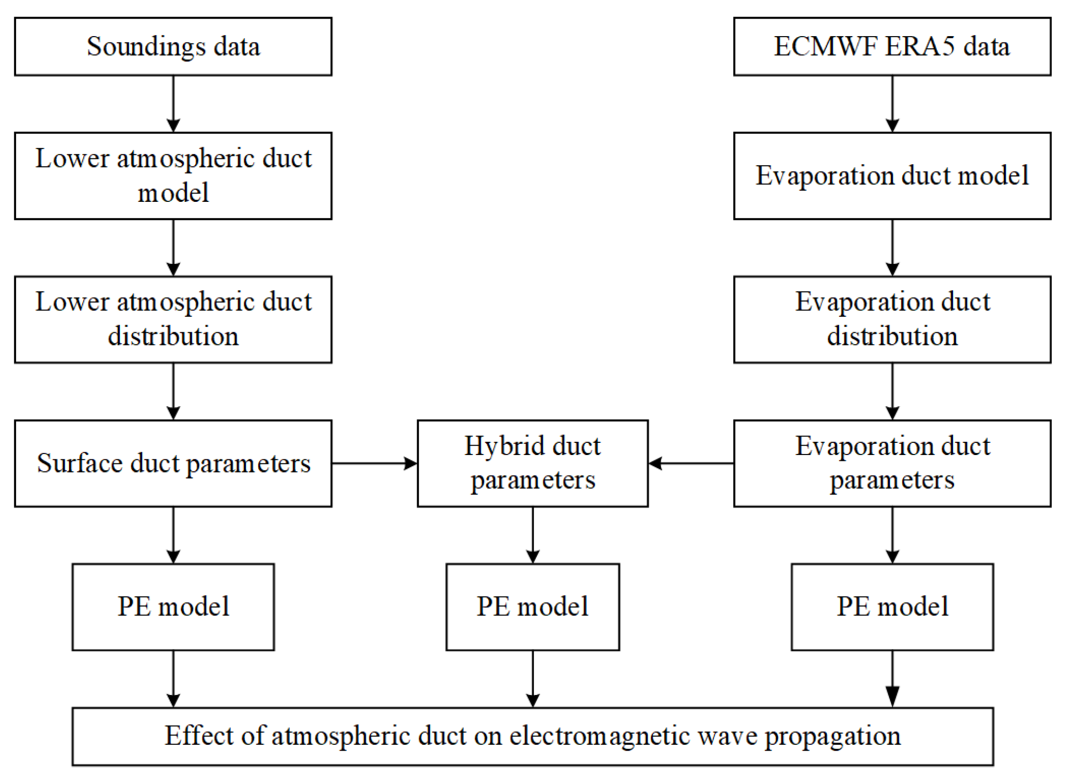
The Bohai Sea and Yellow Sea regions host several significant ports in northern China, such as Tianjin Port, Qingdao Port, and Dalian Port. These ports are crucial for China’s foreign trade, facilitating economic exchanges and cooperation both within the region and internationally. Currently, research on the statistical characteristics of tropospheric waveguides and electromagnetic wave propagation in the near-sea atmosphere of China predominantly focuses on the South China Sea, with relatively limited attention being given to the Yellow Sea and Bohai Sea regions. This study utilizes sounding data from six high-altitude meteorological stations and ECMWF ERA5 reanalysis data to investigate the tropospheric waveguides and electromagnetic wave propagation characteristics in the Yellow Sea and Bohai Sea regions. The structure of this paper is as follows: the second part introduces the data and models used; the third part analyzes the distribution characteristics of atmospheric ducts in the Bohai Sea and Yellow Sea regions; the fourth part presents the propagation characteristics of electromagnetic waves in atmospheric duct environments; finally, the fifth part provides the conclusions (Figure 1).
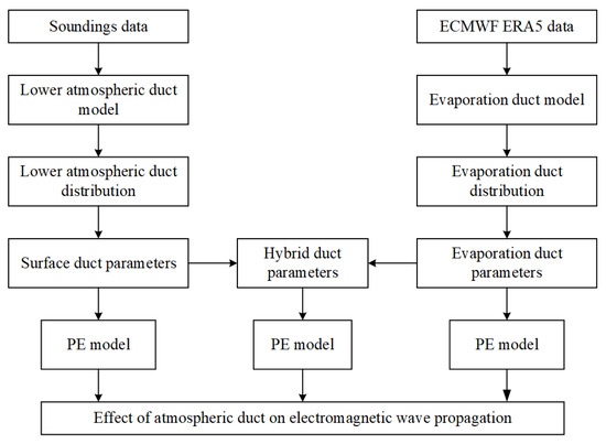
Figure 1.
Flowchart of this study.
2. Materials and Methods
2.1. Data
2.1.1. Sounding Data
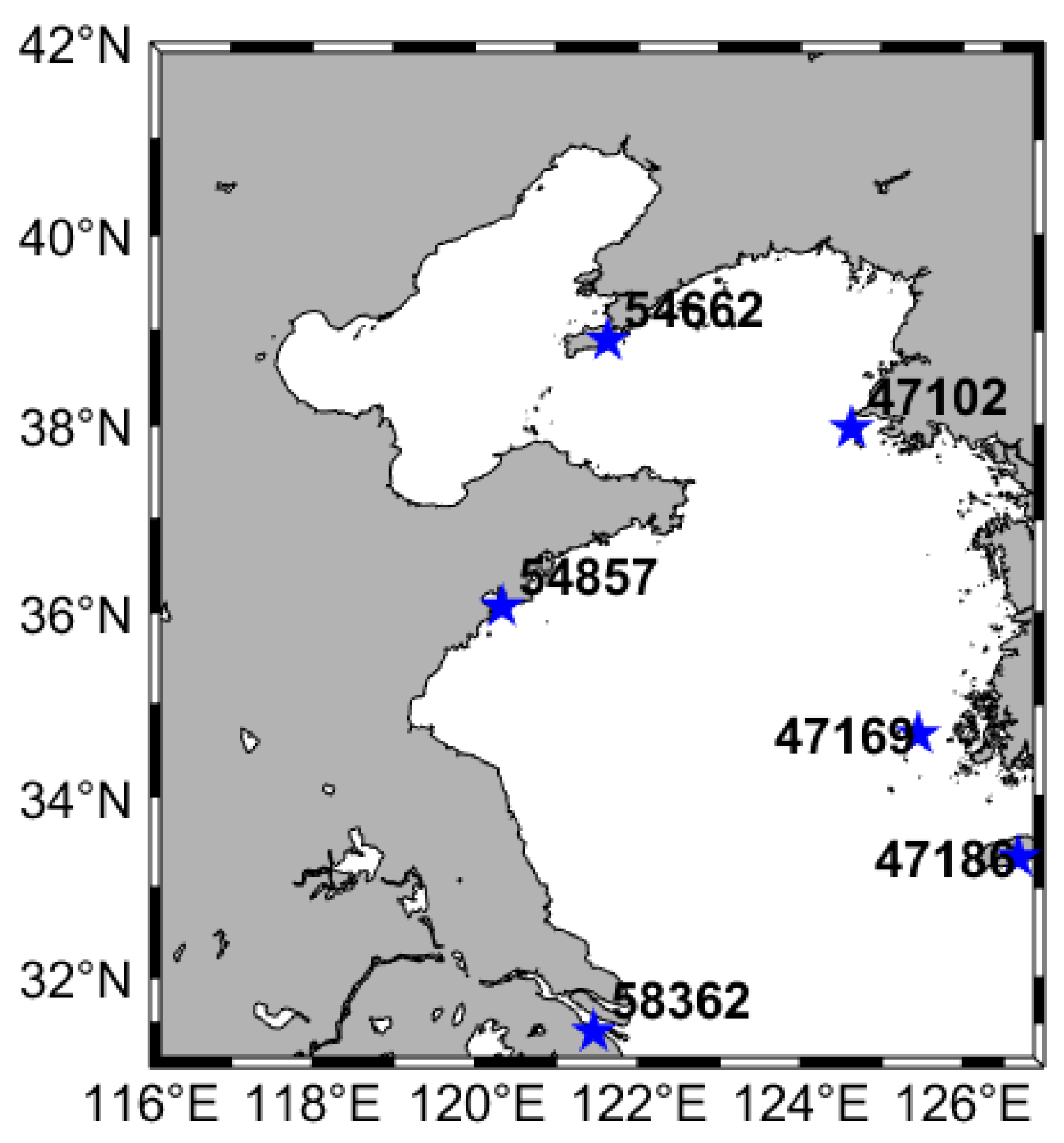
The meteorological sounding data used in this study were sourced from the Wyoming Weather website. These data cover high-resolution vertical structure information on atmospheric elements, such as temperature, pressure, and humidity. This information can be used for the statistical analysis of lower atmospheric ducts. Specifically, this study utilizes data from six upper-air meteorological stations. The locations of these stations are shown in Figure 2, and detailed information for each station is listed in Table 1.
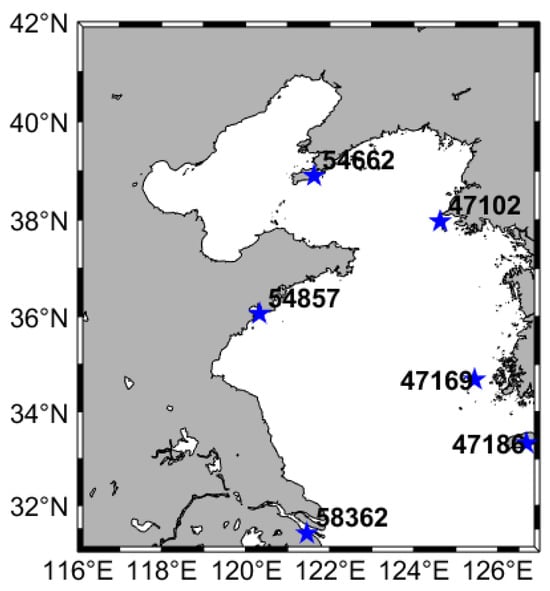
Figure 2.
The study area (blue stars denote meteorological station locations; image sourced from the MATLAB software).

Table 1.
Information on meteorological sounding data.
2.1.2. Reanalysis Data
This study utilizes ECMWF ERA5 reanalysis data to analyze the distribution characteristics of evaporation ducts in the Bohai Sea and Yellow Sea regions. The ECMWF ERA5 dataset [32], produced by the European Center for Medium-Range Weather Forecasts (ECMWF) through its Integrated Forecasting System (IFS), is a fifth-generation global climate reanalysis dataset. It offers a spatial resolution of up to 31 km and a temporal resolution on an hourly basis. This high resolution allows the dataset to comprehensively describe the spatiotemporal variations in meteorological elements. Researchers have validated the accuracy of ERA5 reanalysis data through lower atmospheric refractivity curve observation experiments over the East China Sea [10]. The study area selected for this study spans from 116° E to 127° E in longitude and 31° N to 42° N in latitude, covering the period from 2017 to 2019. Detailed information on the meteorological parameters used in this study is provided in Table 2.
Table 2.
Meteorological variables from the ERA5 reanalysis data used in this study.
2.2. Atmospheric Duct Model
The refractive characteristics of electromagnetic waves in the troposphere are typically described using the atmospheric refractive index n. The value of n depends on meteorological variables such as temperature, humidity, and pressure. Since the meteorological fields in the actual troposphere are non-uniform, the atmospheric refractive index n varies with altitude and distance. In the lower atmosphere, its values generally range from 1.00025 to 1.00040 [33]. Although the changes are very slight, they still produce significant refraction effects on electromagnetic waves, with the degree of refraction mainly depending on the gradient of changes in n along the propagation path. To facilitate the description of these minor variations and their impacts on electromagnetic wave propagation calculations, the atmospheric refractivity N is often used to describe the refraction effect of the atmosphere [33] and is defined as
where the unit of N is referred to as N-units. According to Bean and Dutton [34], based on the Debye theory [35], the relationships between N and the atmospheric temperature T (K), pressure P (mb), and water vapor pressure e (mb) are given by
where represents the atmospheric relative humidity (%). When considering the curvature of the Earth, the corrected refractive index can be expressed as follows [36]:
where h represents the height above the ground (km), and a represents the radius of the Earth, which is taken to be 6371 km.
The propagation path of electromagnetic waves in the troposphere mainly depends on the gradient of the corrected refractive index. When the gradient is in M-units/m, the curvature of the electromagnetic wave rays will be less than the curvature of the Earth. As a result, the electromagnetic waves become trapped within a certain thickness of the atmospheric layer, propagating within this layer. This refractive environment is referred to as a trapping refractive environment, and the corresponding atmospheric layer is known as a tropospheric duct.
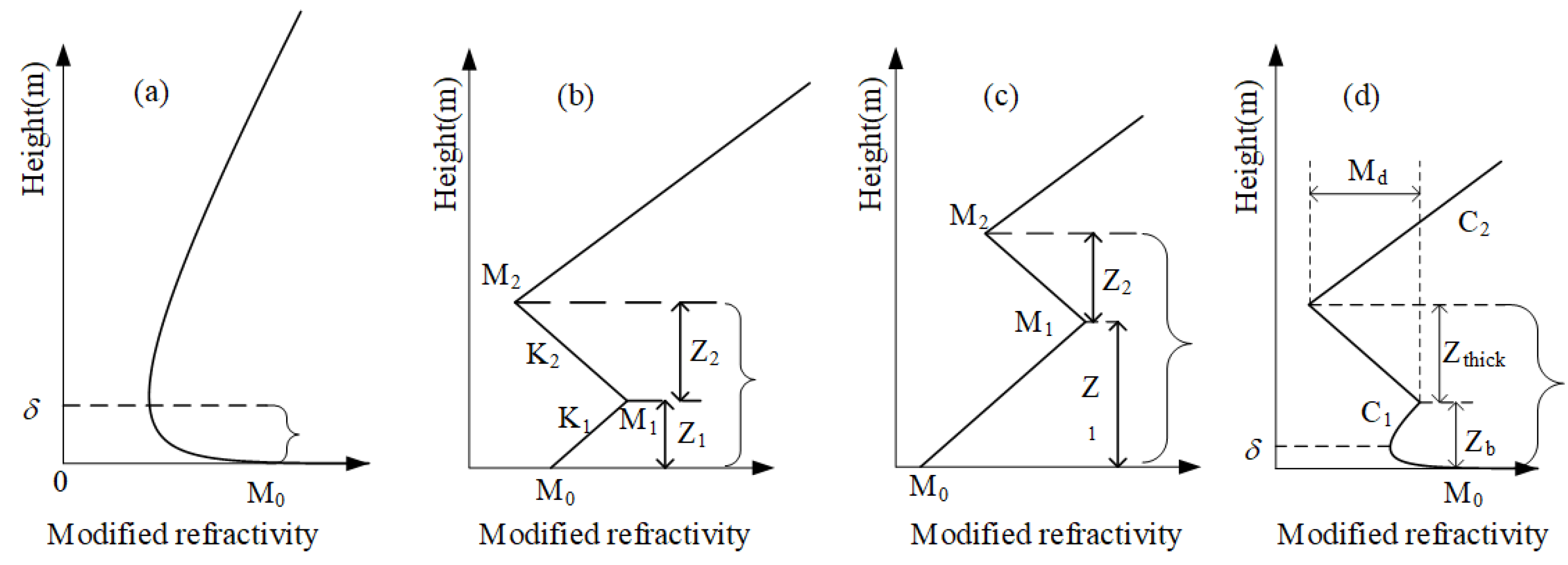
Tropospheric ducts are primarily categorized into three types: evaporation ducts, surface ducts, and elevated ducts, in addition to mixed ducts formed by evaporation and surface ducts. The corresponding spatial structures and parameters are illustrated in Figure 3.
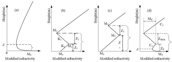
Figure 3.
Different types of atmospheric ducts: (a) evaporation duct, (b) surface duct, (c) elevated duct, and (d) hybrid duct.
The structural parameters of a duct include the duct top height, duct bottom height, duct thickness, and duct strength. Duct strength and duct thickness are crucial factors in determining whether electromagnetic waves will be trapped within the duct.
2.2.1. Lower Atmospheric Ducts
The models for surface ducts and elevated ducts are represented as follows [36]:
where and represent the height of the duct base layer and the thickness of the waveguide trapping layer, respectively. and represent the slopes of the duct’s substrate layer and cladding layer, respectively. represents the corrected refractive index at the sea-surface height; , .
The hybrid duct model is represented as follows [37]:
where represents the evaporation duct height, represents the gradient of the mixed layer, represents the base height of the trapping layer, represents the thickness of the trapping layer, and represents the strength of the trapping layer, which typically ranges from 0 to 100 M-units. Additionally, represents the aerodynamic roughness factor, typically taken as m; is the neutral-stratification evaporation duct parameter, typically M-units/m; is the modified refractive index gradient above the trapping layer, usually taken as M-units/m under standard atmospheric conditions; is the height distinguishing an evaporation duct from a surface duct, which can be calculated using the following formula:
where represents the height of the top of the duct trapping layer, and . is calculated using the following formula:
2.2.2. Evaporation Duct Model
The modified refractive index profile of the evaporation duct under neutral stratification is represented as follows [38]:
where z represents the vertical height above the sea surface; is the aerodynamic roughness factor, typically taken as m; is the height of the evaporation duct, and is the atmospheric modified refractive index at sea level.
2.3. Evaporation Duct Diagnostic Model
Due to the difficulty of directly obtaining the refractive index profile in the vertical direction near the sea surface, most existing evaporation duct models use several meteorological parameters at heights near the sea surface as input. Examples of such models include the Paulus–Jeske (PJ) model [39], the Musson–Gauthier–Bruth (MGB) model [40], the Babin–Young–Carton (BYC) model [41], and the NPS model [14]. S. M. Babin et al. [14,41,42] compared the P-J, MGB, BYC, and NPS models using profile data measured by buoys and concluded that the BYC and NPS models perform best. Guo Xiangming et al. [43] compared the PJ model proposed by Paulus and the NPS model based on approximately seven months of hydrometeorological data measured on offshore platforms. Their study indicated that the NPS model predicts propagation loss better than the PJ model, especially under unstable atmospheric conditions. Therefore, this study selects the NPS model based on the COARE 3.0 algorithm for calculating the modified atmospheric refractive index profile.
In the NPS model, the vertical profiles of specific humidity q and temperature T are represented as follows [41,42]:
where and represent the specific humidity and atmospheric temperature at a given height, respectively; and represent the sea-surface specific humidity and temperature after salinity correction; and represent the sea-surface saturation specific humidity; and represent the characteristic scales for specific humidity q and potential temperature , respectively; L is the similarity length; is the dry adiabatic lapse rate ( K/m); is the von Karman constant, typically valued at 0.4; is the roughness length corresponding to the water temperature; is the universal function. The NPS model originally used the COARE 2.6 algorithm. In this study, the COARE 3.0 algorithm is employed to calculate the sea-surface roughness and surface-layer scale parameters. By combining the ideal gas law with the hydrostatic equation and integrating, we obtain the following [42]:
where is the gas constant for dry air (287.1 J/kg/K), and is the mean virtual temperature at heights and .
Through the conversion relationship between the water vapor pressure e and specific humidity q, the vertical distribution profile of water vapor pressure can be obtained as follows [44]:
Finally, by combining the temperature, atmospheric pressure, and water vapor pressure profiles obtained from Equations (11)–(14) with the atmospheric modified refractive index formula, the profile can be obtained. The evaporation duct height corresponds to the height at which the modified refractive index profile reaches its minimum value.
2.4. Parabolic Equation Model
In a two-dimensional Cartesian coordinate system, assuming that the electromagnetic wave propagates along the x-axis and that the electromagnetic field components are independent of the y-axis, the field component satisfies the following two-dimensional scalar wave equation under the condition that the refractive index of the propagation medium n is isotropic [45]:
where represents the wavenumber of the electromagnetic wave in a vacuum; for the propagation of radio waves over a flat surface, x denotes the horizontal distance, z represents the height above the ground, and represents the electric or magnetic field component.
Since we are primarily concerned with the propagation of electromagnetic wave energy in the paraxial direction, specifically, the variation in the amplitude of the electric/magnetic field, rather than the phase change with distance, we can introduce a simplified function to characterize the amplitude variation of the electric or magnetic field component, as shown in the following equation [46]:
Substituting Equation (16) into Equation (15) yields a simplified two-dimensional scalar wave equation satisfied by as follows [46]:
Since this study only considers the forward propagation of electromagnetic waves in the tropospheric waveguide, we will only discuss the solution of the forward parabolic equation. Further derivation of Equation (17) yields the following forward narrow-angle parabolic equation [46]:
For Equation (18), there are currently two main methods of solution: the split-step Fourier transform (SSFT) method and the finite difference method [45]. The SSFT method is a numerical method for solving parabolic equations in the spectral domain. It can easily account for horizontally inhomogeneous refractive indices and, compared to the finite difference method, has very lenient constraints on the step size , allowing for larger values. This makes it suitable for calculating long-distance wave propagation characteristics. Reference [46] provides a detailed description of the SSFT solution process for the PE equation.
The hardware platform utilized in this study was a laptop equipped with 8 GB of RAM and a CORE i5 processor. The data processing was performed using the Python software 3.12.3, while the computational experiments were conducted using the MATLAB software 9.10.
3. Results and Discussion
3.1. Analysis of Atmospheric Duct Distribution Characteristics in the Bohai Sea and Yellow Sea
3.1.1. Distribution Characteristics of Lower Atmospheric Ducts
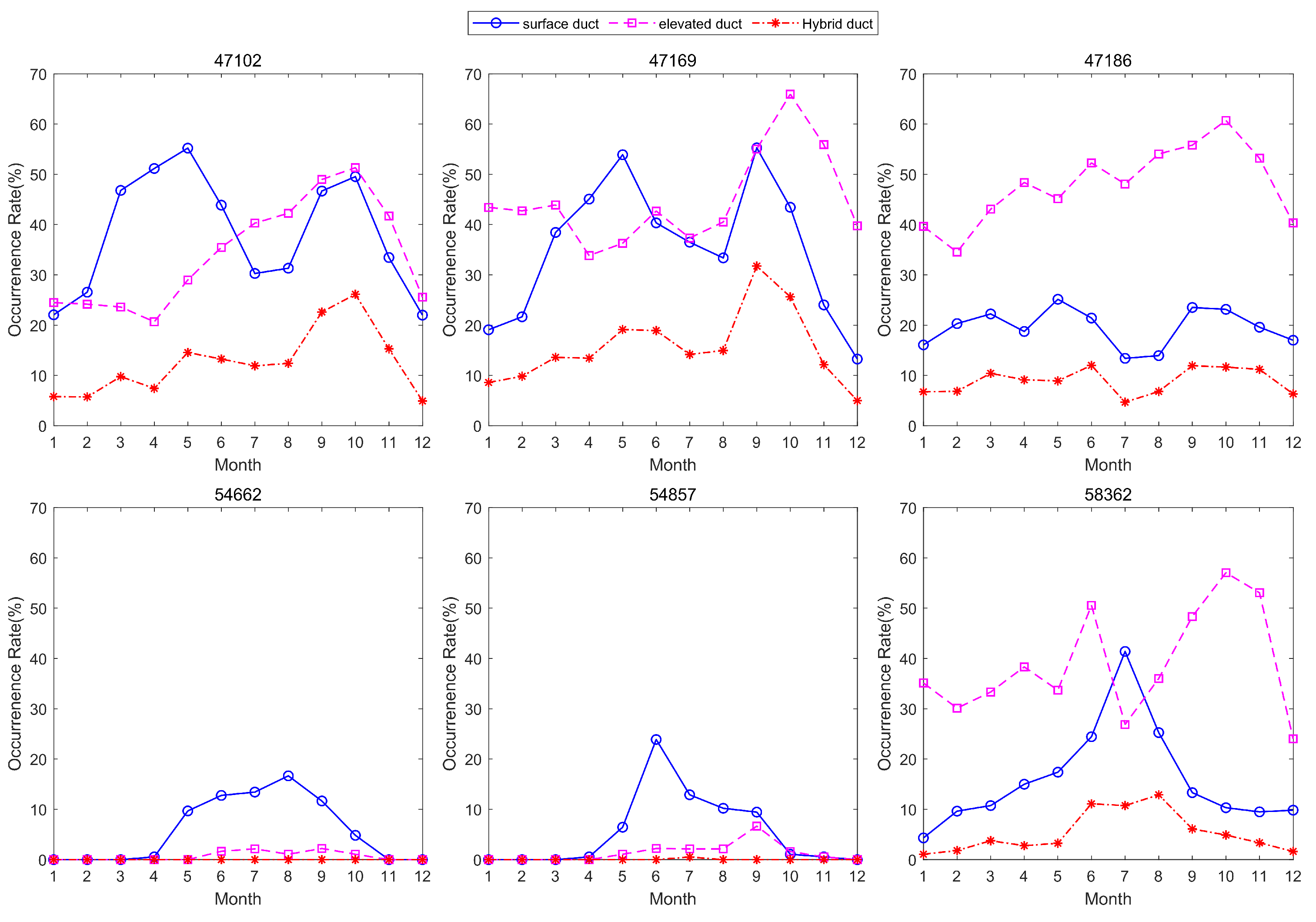
In this section, the distribution characteristics of lower atmospheric ducts in the Bohai Sea and Yellow Sea regions are analyzed using sounding data from six upper-air meteorological stations. Figure 4 shows the monthly average occurrence rates of surface ducts and elevated ducts at the six meteorological stations. Table 3 presents the characteristic parameters of surface ducts and elevated ducts.
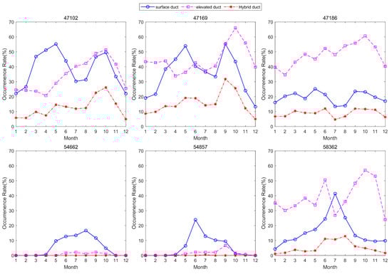
Figure 4.
Monthly average occurrence rates of surface ducts and elevated ducts at meteorological stations.
Table 3.
Characteristic parameters of surface ducts and elevated ducts.
As shown in Figure 4, the occurrence rate of surface ducts is higher from May to September, primarily due to the prevalence of the East Asian summer monsoon, which brings higher temperatures and humidity. When warm, moist air flows over cooler water bodies, it causes temperature and humidity inversions, leading to the formation of ducts in the upper part of the marine atmospheric boundary layer. Conversely, from October to April of the following year, the occurrence rate of surface ducts is lower. This is mainly because the region gradually comes under the control of high pressure induced by continental cold air, with the winter monsoon reducing atmospheric humidity, which is unfavorable for duct formation. The monthly average distribution of surface ducts at stations 47,102, 47,169, and 47,186 shows an “M” shape, possibly because the height of surface ducts decreases in summer, making it undetectable by the meteorological stations. Additionally, the occurrence rate of elevated ducts peaks in October, reaching up to 60%.
Due to the insufficient vertical resolution at stations 54,662 and 54,857, the thickness of the surface ducts and elevated ducts at these stations is significantly greater than that at other stations. The base height of the surface ducts ranges from 46.8 m to 237.9 m, with duct strengths between 6.1 M-units and 9.3 M-units. The duct thickness is relatively consistent, approximately 50 m. The base height of the elevated ducts ranges from about 1100 m to 1300 m, with duct strengths between 8 M-units and 10 M-units and a thickness of around 90 m.
3.1.2. Distribution Characteristics of Evaporation Ducts
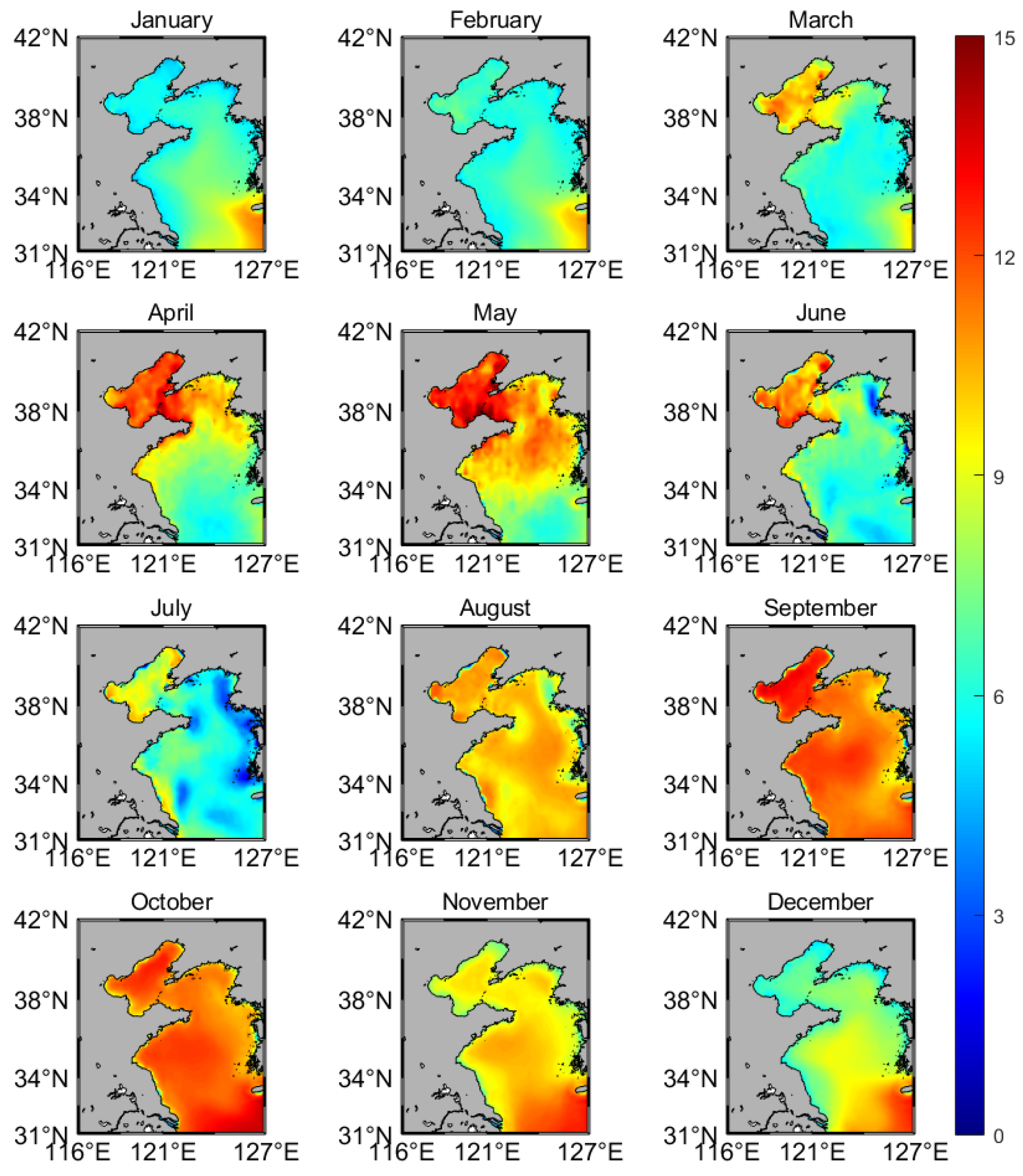
In this section, the evaporation duct height in the Yellow and Bohai Sea regions was obtained using ECMWF ERA5 reanalysis data through an evaporation duct diagnostic model. Figure 5 shows the distribution of the monthly average evaporation duct height in the Yellow and Bohai Sea regions.
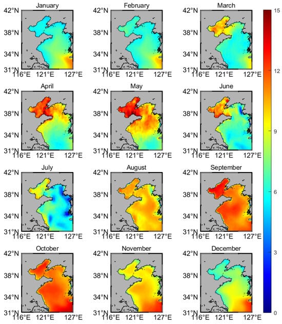
Figure 5.
Distribution of the monthly average evaporation duct height in the Yellow and Bohai Sea regions.
As shown in Figure 5, the evaporation duct height distribution in the Yellow and Bohai Seas region varies over time. From November to February of the following year, the evaporation duct height exhibits a pattern of being higher in the southeast and lower in the northwest. From March to May, the evaporation duct height in the northern region gradually increases and extends southward, showing a pattern of being higher in the south and lower in the north. From June to October, the evaporation duct height increases, and the distribution becomes more uniform. In the Bohai Sea region, the evaporation duct height peaks in April, May, September, and October, reaching up to 13 m, while it is at its lowest in January and February, at only 6 m, which is consistent with the findings in [47]. In the Yellow Sea region, the evaporation duct height reaches its maximum in September and October at 12 m and its minimum in June and July at 7 m.
3.2. Electromagnetic Wave Propagation Characteristics in Atmospheric Ducting Environments
This section will discuss the electromagnetic wave propagation characteristics in evaporation duct, surface duct, and mixed duct environments. Additionally, it will analyze the impacts of electromagnetic wave frequency and antenna height (AH) on the propagation loss in atmospheric ducting environments.
3.2.1. Electromagnetic Wave Propagation Characteristics in Evaporation Duct Environments
In this subsection, the evaporation duct data from the Yellow and Bohai Sea regions in Section 3.2 is used to analyze the electromagnetic wave propagation characteristics in evaporation duct environments through the PE equation. Given that both uniform and non-uniform evaporation ducts exist in the Yellow and Bohai Sea regions, this subsection will discuss the electromagnetic wave propagation characteristics in these two environments separately.
We use the average evaporation duct height data for May from Figure 5, setting a non-uniform evaporation duct height (starting point at (35° N, 124° E) and ending point at (33° N, 124° E)), while the uniform evaporation duct height is set to 10.5 m. The vertical profile of the uniform evaporation duct, the height of the non-uniform evaporation duct, and the corresponding propagation loss distribution are shown in Figure 6. The parameter settings for the PE equation are shown in Table 4, where the antenna height is set to 5 m to ensure that the antenna is located within the duct layer of the evaporation duct.
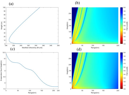
Figure 6.
Vertical profile of a uniform evaporation duct (a), height of a non-uniform evaporation duct (b), and the corresponding propagation loss (c,d).
Table 4.
Parameters for the PE model.
As shown in Figure 6c, the evaporation duct heights at the starting and ending points are 10.5 m and 7.7 m, respectively, with the height gradually decreasing with distance. By observing Figure 6b,d, we find a strip of a low-propagation-loss region within the duct layer in both figures. It is noteworthy that the low-propagation-loss region in the non-uniform evaporation duct environment in Figure 6d is significantly shorter.
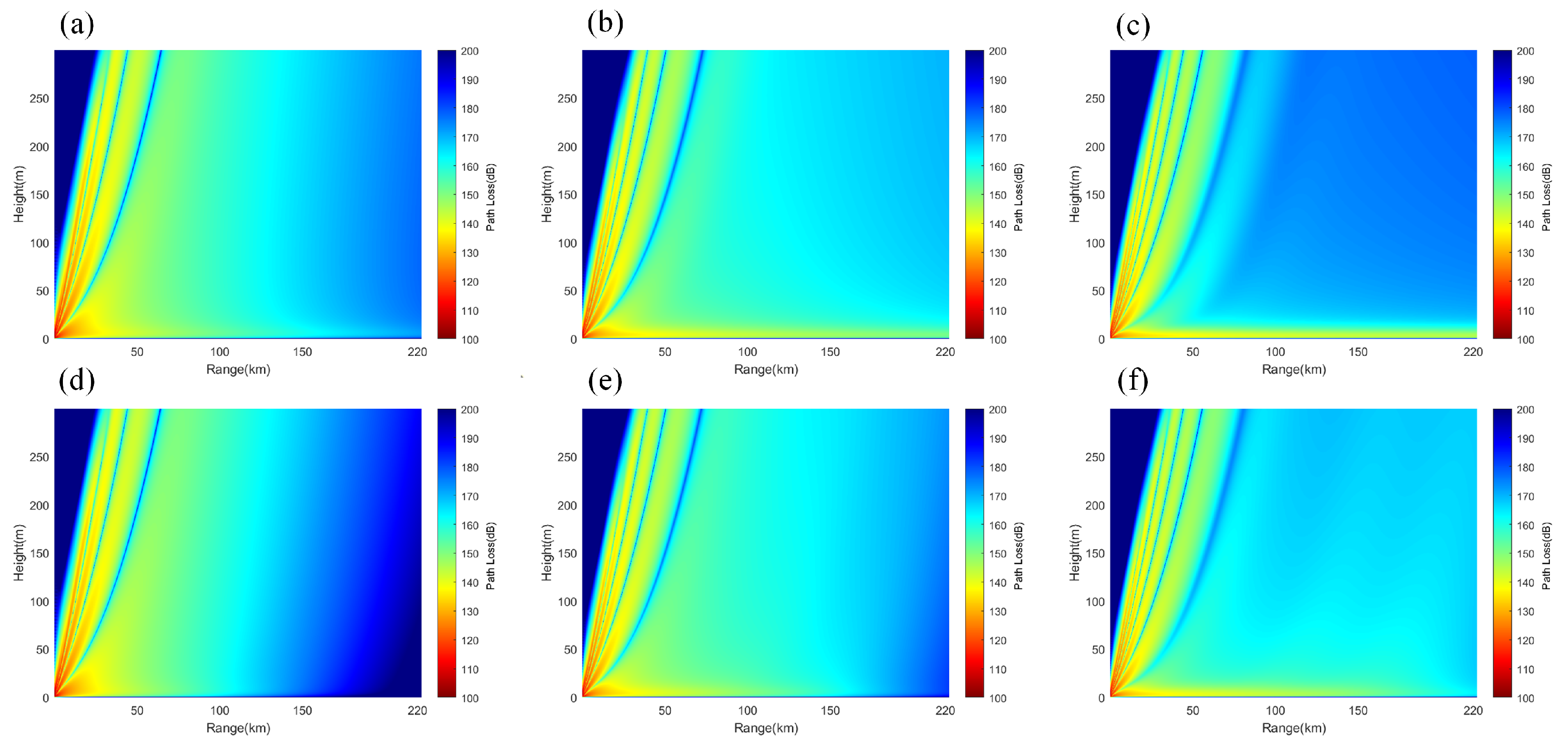
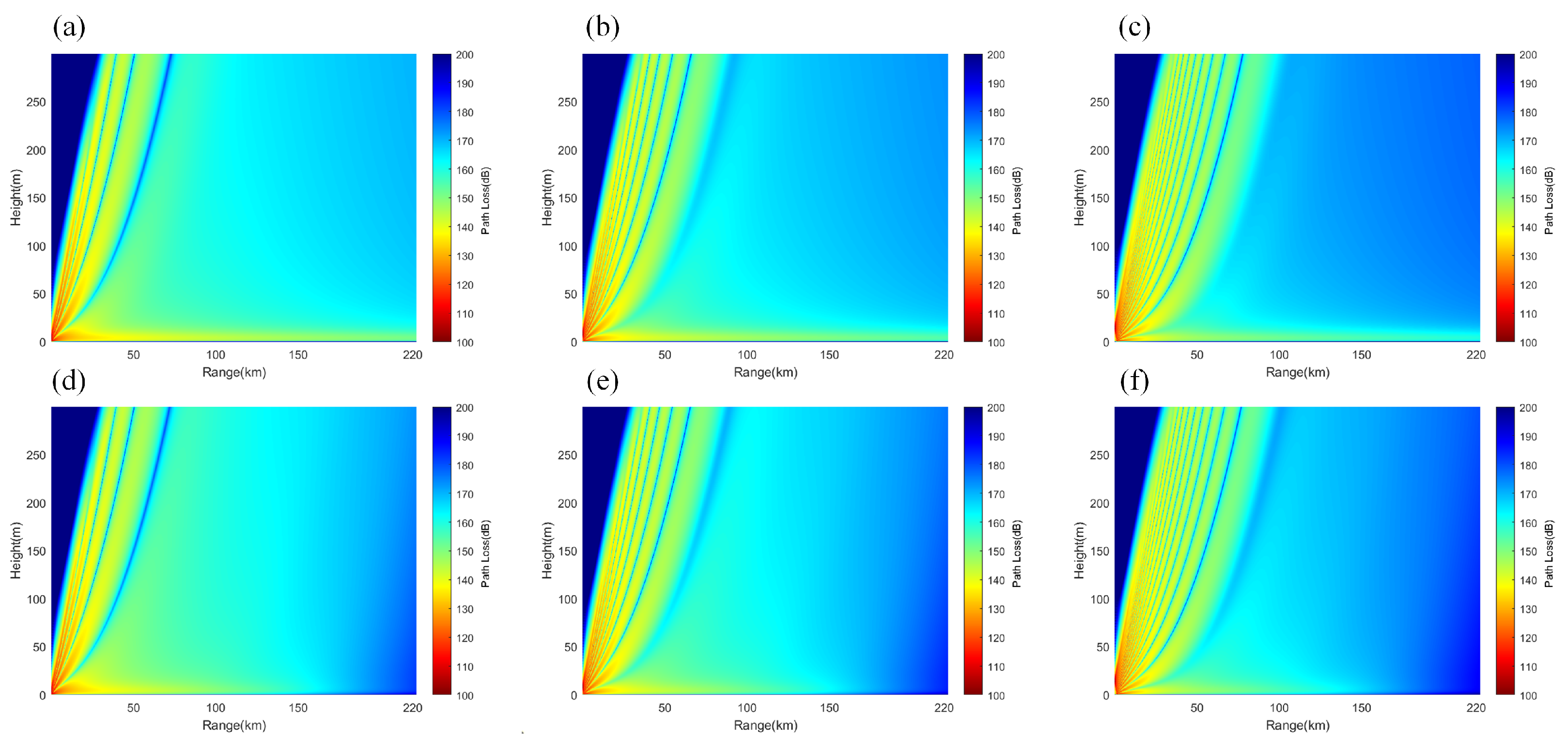
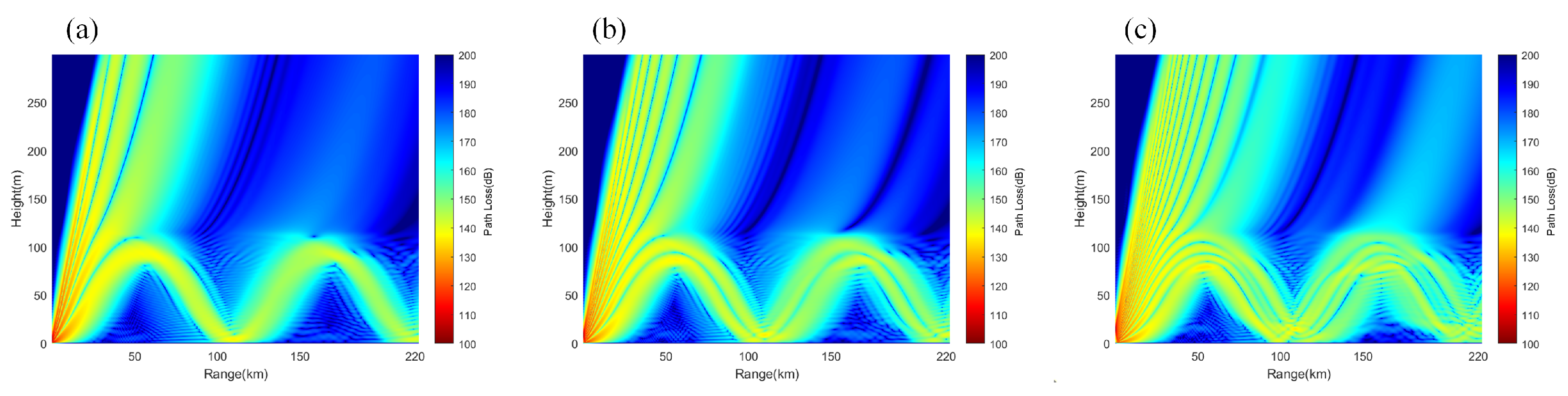
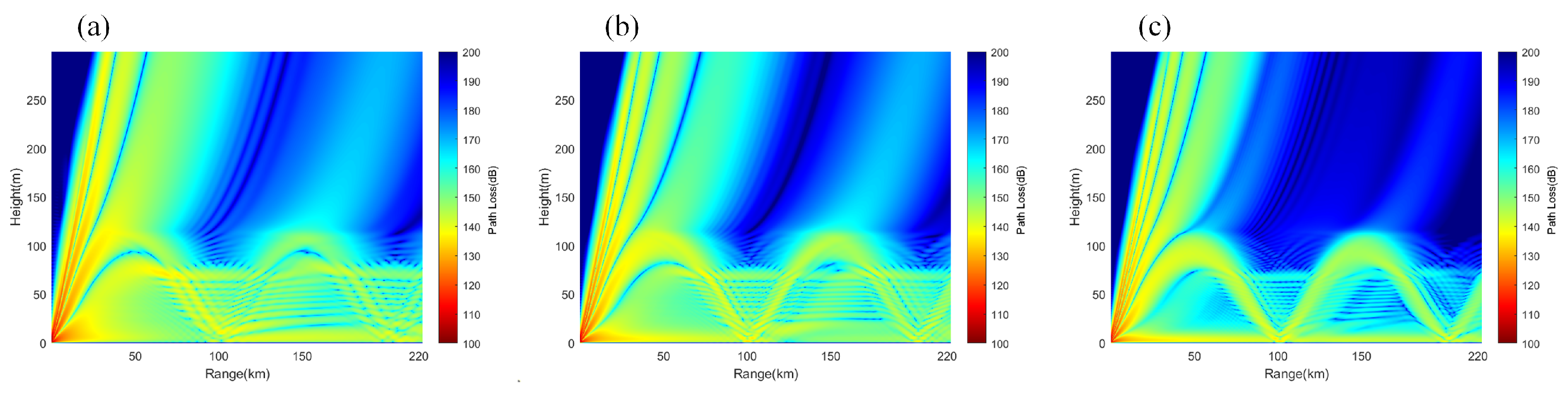
As shown in Figure 7, with the increase in electromagnetic wave frequency, more electromagnetic waves are trapped within the duct layer in a uniform evaporation duct environment, forming a shadow region above the duct layer. In contrast, in a non-uniform evaporation duct environment, the low-propagation-loss region extends forward.

Figure 7.
(a–c) represent the propagation loss of electromagnetic waves at frequencies of 12 GHz, 15 GHz, and 18 GHz in a uniform evaporation duct environment, respectively. (d–f) represent the propagation loss of electromagnetic waves at frequencies of 12 GHz, 15 GHz, and 18 GHz in a non-uniform evaporation duct environment, respectively.
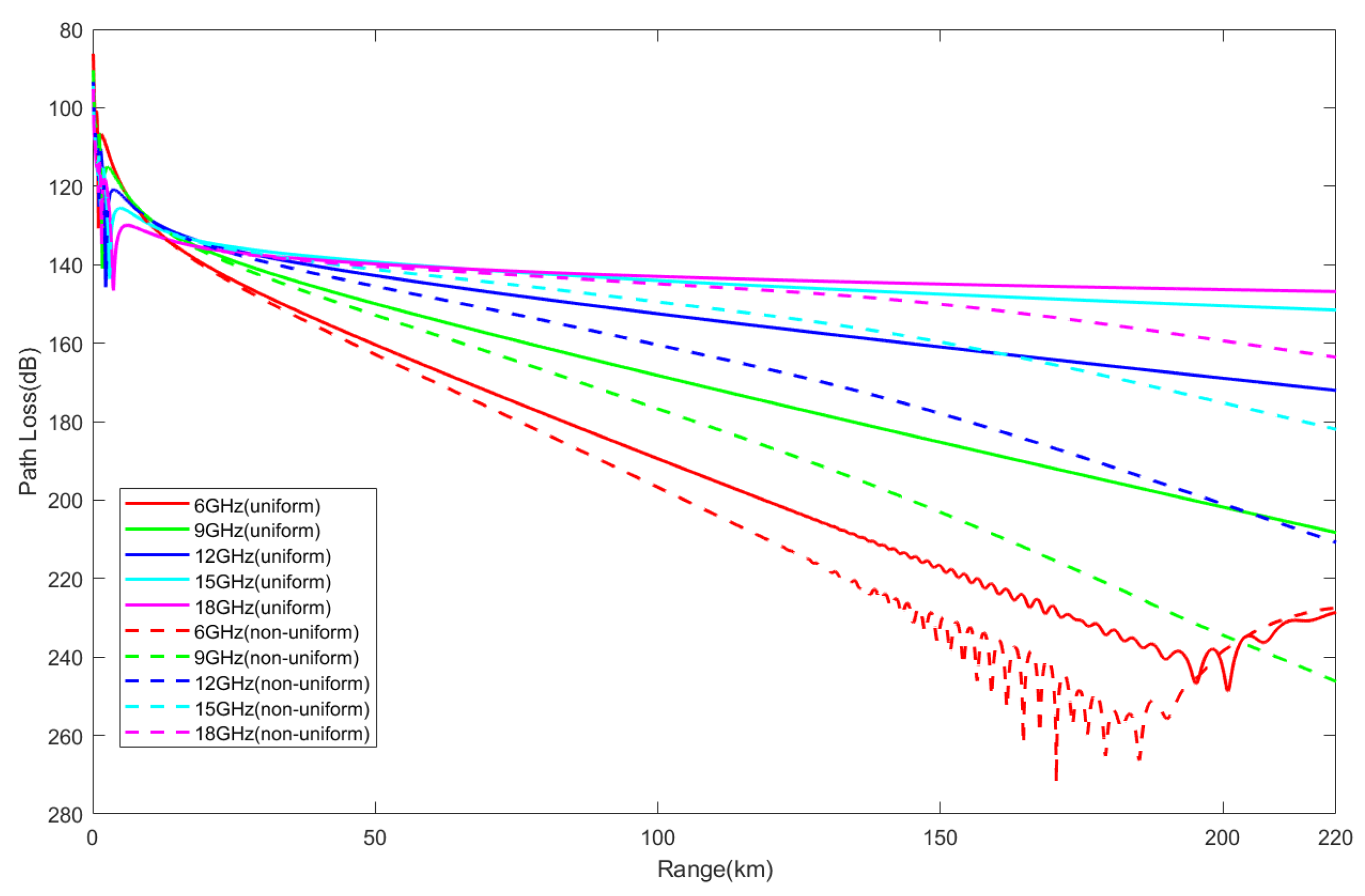
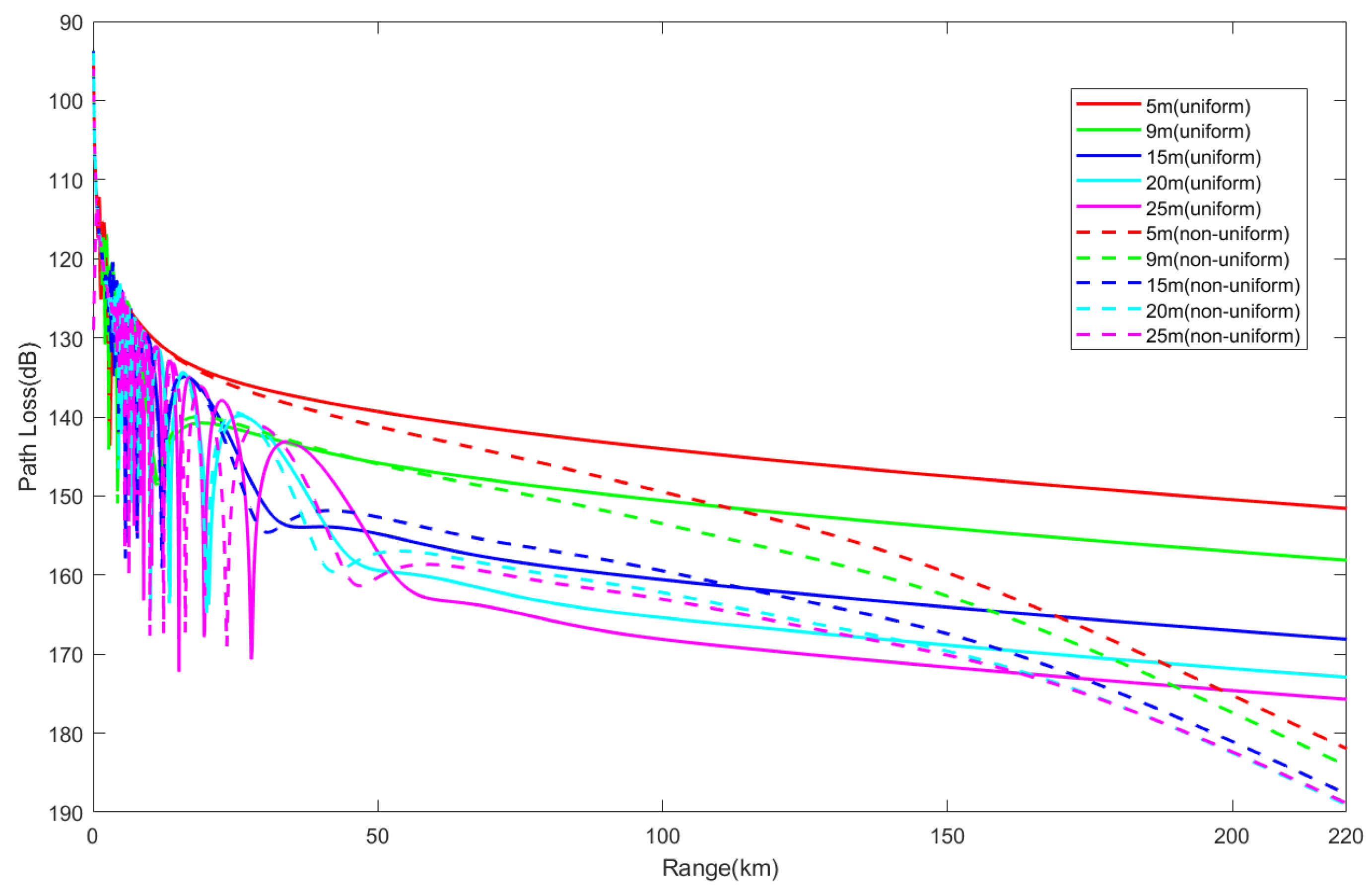
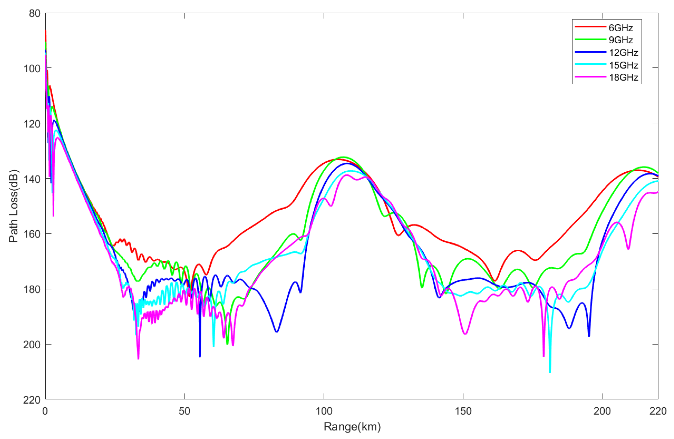
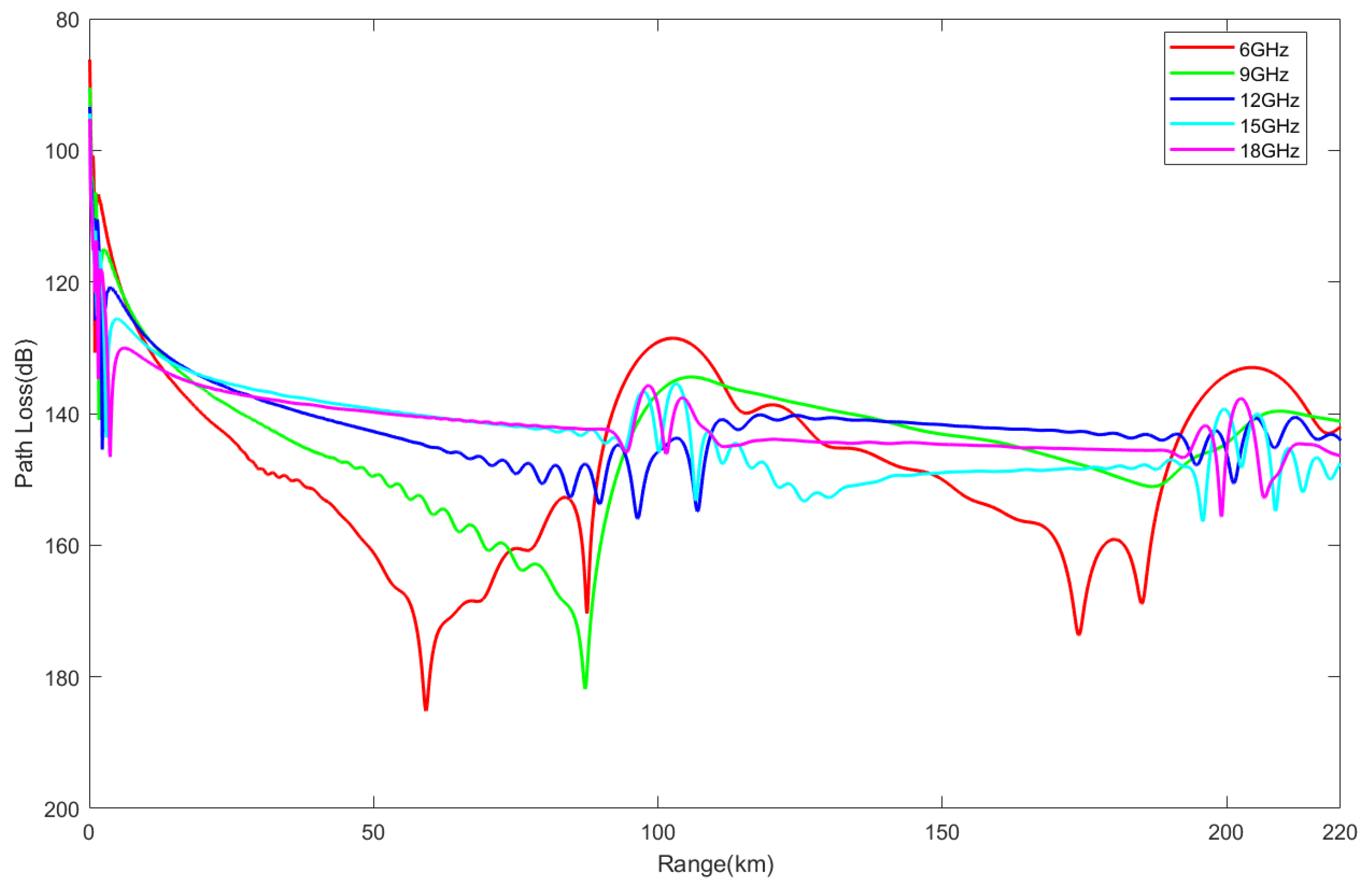
As shown in Figure 8, when the electromagnetic wave frequency is 6 GHz, the propagation loss begins to fluctuate at 136 km. The amplitude of propagation loss fluctuations in a non-uniform evaporation duct environment is greater than that in a uniform evaporation duct environment. This indicates that the electromagnetic wave in the non-uniform evaporation duct environment has penetrated the duct layer. As the frequency of the electromagnetic wave increases, the propagation loss in both uniform and non-uniform evaporation duct environments decreases and gradually increases smoothly with distance.
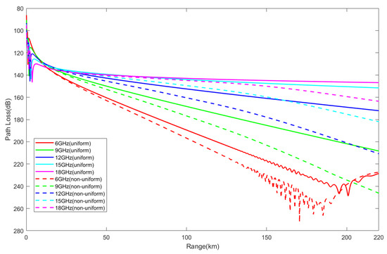
Figure 8.
Variations in the propagation loss with distance for electromagnetic waves of different frequencies in uniform and non-uniform evaporation duct environments.
When the electromagnetic wave frequencies are 12 GHz, 15 GHz, and 18 GHz, the differences in propagation loss at 220 km between uniform and non-uniform evaporation duct environments are 38.7 dB, 30.2 dB, and 16.6 dB, respectively. This indicates that as the electromagnetic wave frequency exceeds a certain value and continues to increase, the difference in propagation loss between uniform and non-uniform evaporation duct environments decreases.
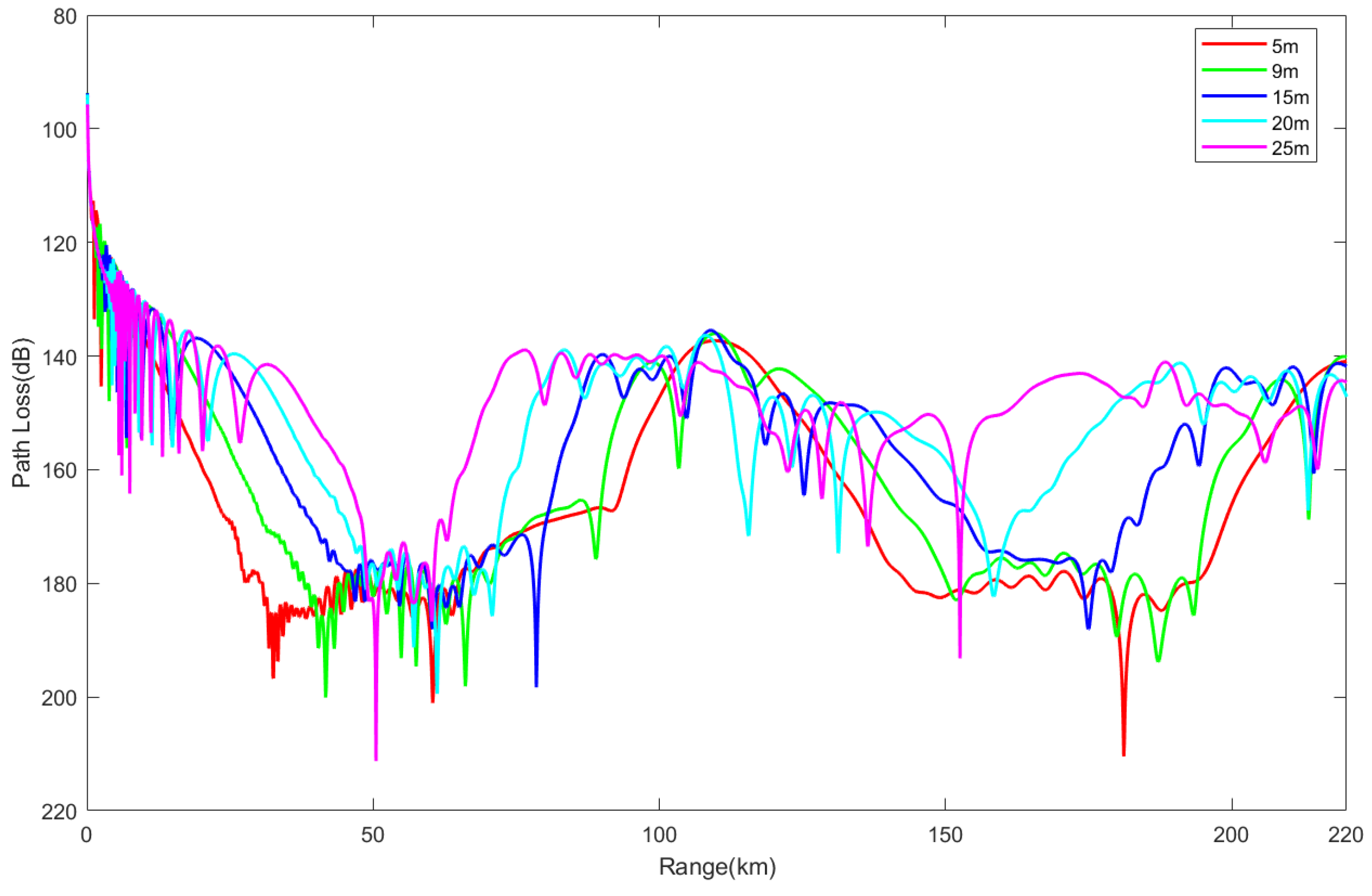
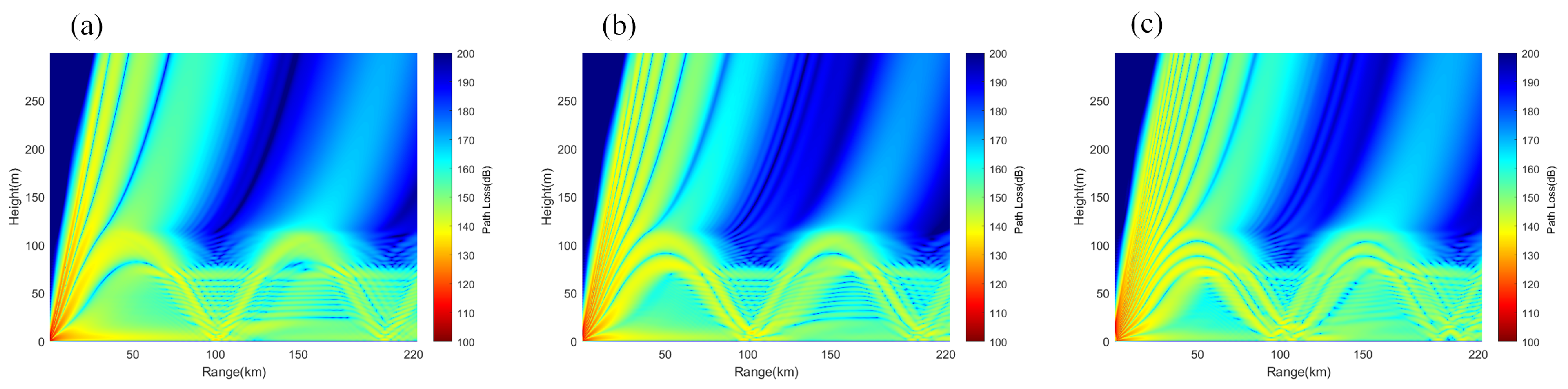
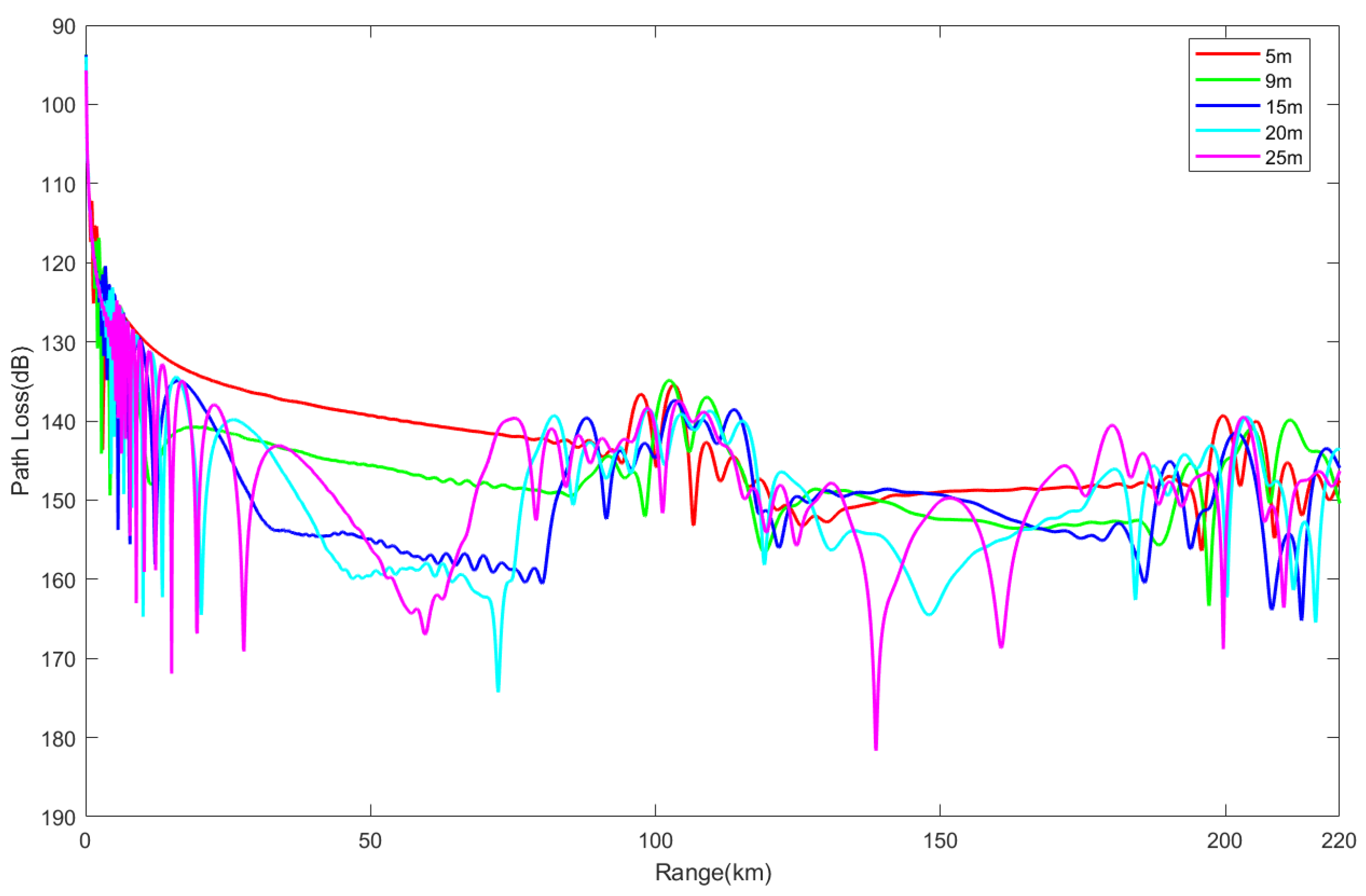
As shown in Figure 9, raising the antenna height expands the low-propagation-loss area above the starting position, indicating that more electromagnetic waves leave the duct layer. Figure 10 shows that increasing antenna height raises the propagation loss in both uniform and non-uniform evaporation duct environments, and fluctuations in propagation loss within a 50-kilometer range also increase.
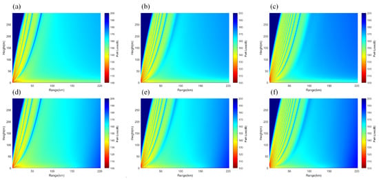
Figure 9.
(a–c) represent the propagation loss at antenna heights of 5 m, 9 m, and 15 m in a uniform evaporation duct environment, respectively. (d–f) represent the propagation loss at antenna heights of 5 m, 9 m, and 15 m in a non-uniform evaporation duct environment, respectively.
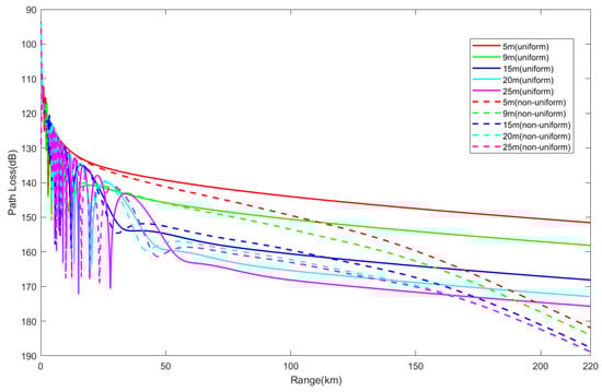
Figure 10.
Variations in the propagation loss with distance for different antenna heights in uniform and non-uniform evaporation duct environments.
3.2.2. Electromagnetic Wave Propagation Characteristics in Surface Duct Environments
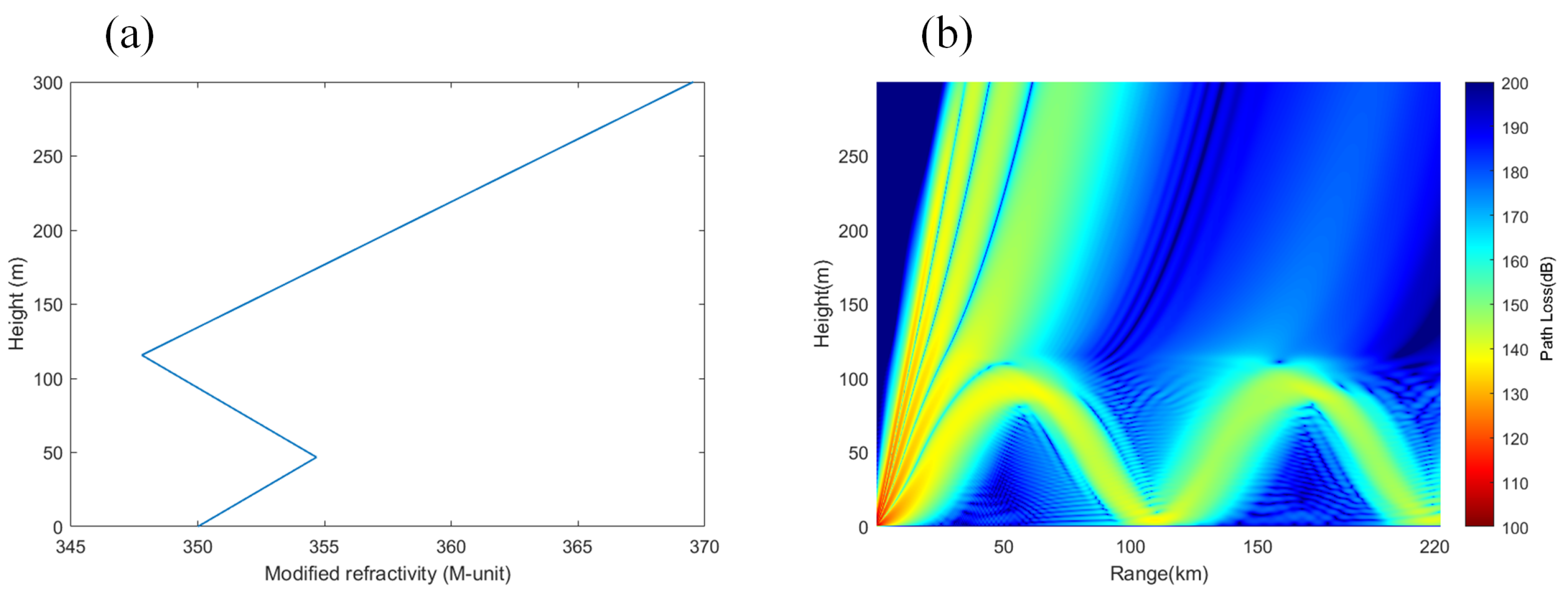
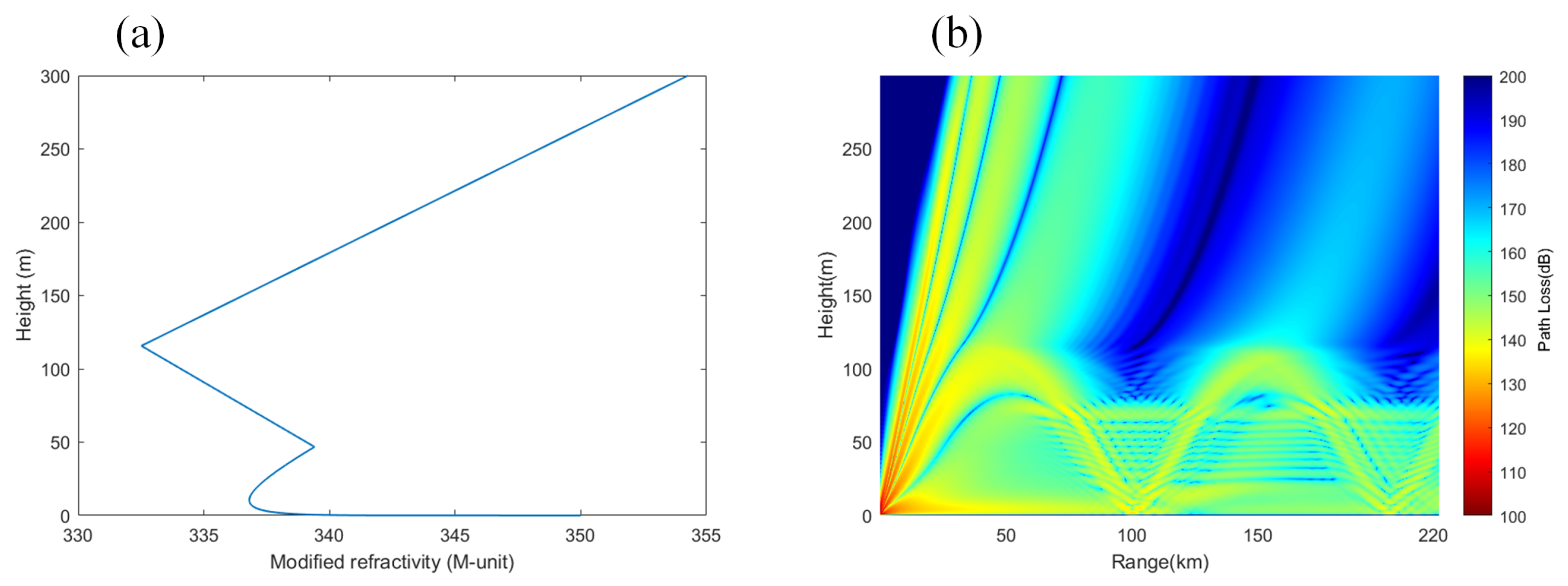
When a surface duct is higher, it has a smaller impact on the electromagnetic wave propagation characteristics near the sea surface. Therefore, in this subsection, the parameters of station 58,362 are used, setting the base height of the surface duct to 46.8 m, the duct thickness to 68.9 m, and the duct strength to 7.1 M-units. The parameters for the PE equation are shown in Table 4. The vertical profile of the surface duct and its propagation loss distribution are shown in Figure 11.

Figure 11.
Vertical profile (a) and propagation loss of surface ducts (b).
As shown in Figure 11b, the low-propagation-loss region within the duct layer in the surface duct environment forms a sinusoidal curve shape, with a peak height of 100 m and a period of 110 km.
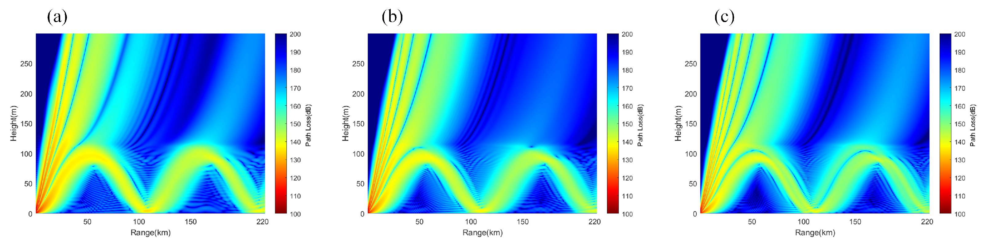
As shown in Figure 12, the frequency of electromagnetic waves has little effect on the distribution of propagation loss in surface duct environments. In Figure 13, as the electromagnetic wave frequency increases, the propagation loss also increases, and the fluctuation amplitude increases, with fluctuation values exceeding 47 dB.

Figure 12.
(a–c) represent the propagation loss of electromagnetic waves at frequencies of 12 GHz, 15 GHz, and 18 GHz in a surface duct environment, respectively.
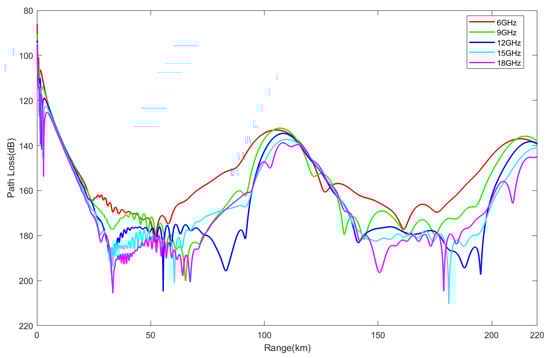
Figure 13.
Variations in the propagation loss with distance for electromagnetic waves of different frequencies in surface duct environments.
As shown in Figure 14, when the antenna height increases, the overall shape of the low-propagation-loss region within the duct layer in the surface duct environment remains sinusoidal, but this region becomes wider. As shown in Figure 15, at different antenna heights, the range of propagation loss varies in roughly the same way, from 140 dB to 200 dB. However, as the antenna height increases, the area with a propagation loss of about 140 dB expands. For example, at an antenna height of 25 m, the propagation loss is around 140 dB, except for areas between 35 to 75 km and a few other small regions. In contrast, at an antenna height of 5 m, only a small region has a propagation loss of 140 dB.
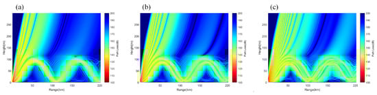
Figure 14.
(a–c) represent the propagation loss at antenna heights of 5 m, 9 m, and 15 m in a surface duct environment, respectively.
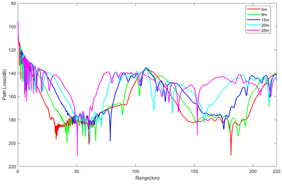
Figure 15.
Variations in propagation loss with distance for different antenna heights in surface duct environments.
3.2.3. Electromagnetic Wave Propagation Characteristics in Hybrid Duct Environments
As known in Section 3.1, the bottom height of the elevated duct in the Yellow–Bohai Sea region is generally around 1200 m, which has a relatively minor effect on the electromagnetic wave propagation loss near the sea surface. The hybrid duct discussed in this subsection refers to the combination of a uniform evaporation duct and a surface duct. The vertical profile of the hybrid duct and its propagation loss distribution are shown in Figure 16.
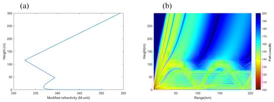
Figure 16.
Vertical profile (a) and propagation loss of the hybrid duct (b).
As shown in Figure 16, the propagation loss distribution in the mixed waveguide environment, based on the evaporation and surface waveguide environments, includes a shaded area from 10 to 70 m.
As shown in Figure 17, with the increase in frequency, more electromagnetic waves are trapped within the waveguide layer of the evaporation duct. Figure 18 illustrates that when the electromagnetic wave frequency is lower (e.g., 6 GHz), the propagation loss fluctuates with increasing distance, similarly to the surface waveguide environment. When the frequency is higher (e.g., 18 GHz), the propagation loss increases gradually with distance, resembling the characteristics of the evaporation duct environment.
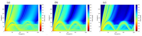
Figure 17.
(a–c) represent the propagation loss of electromagnetic waves in a hybrid duct environment at frequencies of 12 GHz, 15 GHz, and 18 GHz, respectively.
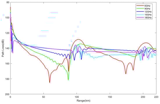
Figure 18.
Propagation loss of electromagnetic waves at different frequencies in a hybrid duct environment as a function of distance.
As shown in Figure 19, with the increase in antenna height, the low-propagation-loss region of the surface waveguide layer in the mixed waveguide becomes wider. Figure 20 indicates that when the antenna is within the waveguide layer of the evaporation duct (AH = 5 m, 9 m), the propagation loss increases with the antenna height. When the antenna is outside the waveguide layer of the evaporation duct (AH = 15 m, 20 m, 25 m), the propagation loss fluctuates between 140 dB and 160 dB. As the antenna height increases, more regions exhibit propagation losses close to 140 dB.
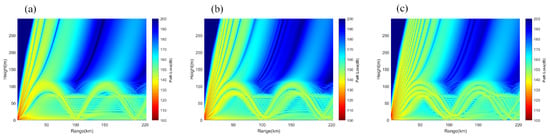
Figure 19.
(a–c) represent the propagation loss in a hybrid duct environment with antenna heights of 5 m, 9 m, and 15 m, respectively.
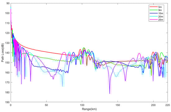
Figure 20.
Propagation loss as a function of distance for different antenna heights in a hybrid duct environment.
In this section, we conduct a detailed analysis of the distribution characteristics of evaporation ducts and lower atmospheric ducts in the Huang–Bohai region. Through parabolic equation simulations, we explore and examine the electromagnetic wave propagation characteristics in different types of atmospheric duct environments. Furthermore, we investigate the impacts of the electromagnetic wave frequency and antenna height on propagation loss in various types of atmospheric duct environments.
4. Conclusions
The atmospheric duct environment significantly affects the propagation of electromagnetic waves. This study utilized sounding data from meteorological stations and ECMWF ERA5 reanalysis data to analyze the distribution characteristics of atmospheric ducts in the Yellow and Bohai Sea regions and explored the impacts of atmospheric duct environments on electromagnetic wave propagation, including the effects of frequency and antenna height using the PE equation. The specific conclusions are as follows:
- Evaporation duct distribution characteristics: In the Bohai Sea region, the height of evaporation ducts is highest in spring and autumn (13 m) and lowest in winter (7 m); in the Yellow Sea region, it is highest in autumn (12 m) and lowest in summer (6 m). The height distribution of ducts in the Yellow Sea is uneven, as it is higher in the southeast and lower in the northwest from November to March, while it is higher in the north and lower in the south in April and May.
- Low-altitude atmospheric duct distribution characteristics: Surface ducts have a higher occurrence rate from May to September and a lower rate from October to April of the following year; elevated ducts have the highest occurrence rate in October (60%).
- Electromagnetic wave propagation characteristics: In an evaporation duct environment, propagation loss increases slowly with distance, and the loss in a non-uniform environment is greater than in a uniform environment; in a surface duct environment, the propagation loss exhibits periodic fluctuations with distance, with fluctuation amplitudes exceeding 47 dB. The propagation loss in a mixed duct environment is between that of evaporation ducts and surface ducts, filling the shadow area from 10 m to 70 m.
- Impacts of frequency and antenna height: In an evaporation duct environment, the higher the frequency and the lower the antenna height, the smaller the propagation loss; in a surface duct environment, the frequency has a smaller impact, but increasing the antenna height widens the low-propagation-loss region. In a mixed duct environment, at low frequencies and antenna heights greater than the evaporation duct height, the propagation characteristics are similar to those of surface ducts; at high frequencies and antenna heights lower than the evaporation duct height, the characteristics are similar to those of evaporation ducts.
This study elucidates the complex effects of atmospheric ducts in the Yellow and Bohai Seas on electromagnetic wave propagation, providing a theoretical basis for related applications. Although this study derived some conclusions regarding the characteristics of atmospheric ducts and electromagnetic wave propagation, it lacks validation through empirical data. Future research directions will involve collaboration with other research institutions to jointly explore the performance of 5G or 6G communications under atmospheric duct conditions through actual measurements and simulation experiments.
Author Contributions
Conceptualization, X.Y. and L.L. (Lei Li); methodology, X.Y. and L.L. (Lei Li); software, X.Y. and L.L. (Lei Li); validation, X.Y., L.L. (Lei Li) and S.L.; formal analysis, X.Y.; investigation, X.Y.; resources, R.Z. and L.L. (Leke Lin); data curation, X.Y.; writing—original draft preparation, X.Y.; writing—review and editing, X.Y. and L.L. (Lei Li); visualization, X.Y.; supervision, Z.Z. and L.L. (Lei Li); project administration, L.L. (Lei Li); funding acquisition, L.L. (Lei Li). All authors have read and agreed to the published version of the manuscript.
Funding
This research was funded by: the National Natural Science Foundation of China, grant number 62101174; Hebei Natural Science Foundation, grant number F2021402005; Science and Technology Project of Hebei Education Department, grant number BJK2022025.
Institutional Review Board Statement
Not applicable.
Informed Consent Statement
Not applicable.
Data Availability Statement
Sounding data: http://weather.uwyo.edu/upperair/sounding.html, accessed on 4 April 2024; ECMWF ERA5 data: https://cds.climate.copernicus.eu/, accessed on 9 April 2024.
Acknowledgments
We thank all of the editors and reviewers for their valuable comments, which greatly improved the presentation of this paper.
Conflicts of Interest
The authors declare no conflicts of interest.
References
- Huang, L.; Zhao, X.; Liu, Y. The Statistical Characteristics of Atmospheric Ducts Observed Over Stations in Different Regions of American Mainland Based on High-Resolution GPS Radiosonde Soundings. Front. Environ. Sci. 2022, 10, 946226. [Google Scholar] [CrossRef]
- Pastore, D.M.; Greenway, D.P.; Stanek, M.J.; Wessinger, S.E.; Haack, T.; Wang, Q.; Hackett, E.E. Comparison of atmospheric refractivity estimation methods and their influence on radar propagation predictions. Radio Sci. 2021, 56, 1–17. [Google Scholar]
- Huang, L.F.; Liu, C.G.; Wang, H.G.; Zhu, Q.L.; Zhang, L.J.; Han, J.; Zhang, Y.S.; Wang, Q.N. Experimental analysis of atmospheric ducts and navigation radar over-the-horizon detection. Remote Sens. 2022, 14, 2588. [Google Scholar] [CrossRef]
- Wang, S.; Yang, K.; Shi, Y.; Zhang, H.; Yang, F.; Hu, D.; Dong, G.; Shu, Y. Long-term over-the-horizon microwave channel measurements and statistical analysis in evaporation ducts over the Yellow Sea. Front. Mar. Sci. 2023, 10, 1077470. [Google Scholar] [CrossRef]
- Yang, C.; Wang, J.; Ma, J. Exploration of X-band communication for maritime applications in the South China Sea. IEEE Antennas Wirel. Propag. Lett. 2021, 21, 481–485. [Google Scholar] [CrossRef]
- Yang, C.; Wang, J. The investigation of cooperation diversity for communication exploiting evaporation ducts in the South China Sea. IEEE Trans. Antennas Propag. 2022, 70, 8337–8347. [Google Scholar] [CrossRef]
- Robinson, L.; Newe, T.; Burke, J.; Toal, D. A simulated and experimental analysis of evaporation duct effects on microwave communications in the Irish Sea. IEEE Trans. Antennas Propag. 2022, 70, 4728–4737. [Google Scholar] [CrossRef]
- Ma, J.; Wang, J.; Yang, C. Long-range microwave links guided by evaporation ducts. IEEE Commun. Mag. 2022, 60, 68–72. [Google Scholar] [CrossRef]
- Zhang, Q.; Wang, S.; Shi, Y.; Yang, K. Measurements and analysis of maritime wireless channel at 8 GHz in the South China Sea region. IEEE Trans. Antennas Propag. 2022, 71, 2674–2681. [Google Scholar] [CrossRef]
- Qiu, Z.; Zhang, C.; Wang, B.; Hu, T.; Zou, J.; Li, Z.; Chen, S.; Wu, S. Analysis of the accuracy of using ERA5 reanalysis data for diagnosis of evaporation ducts in the East China Sea. Front. Mar. Sci. 2023, 9, 1108600. [Google Scholar] [CrossRef]
- Shi, Y.; Yang, K.; Yang, Y.; Ma, Y. A new evaporation duct climatology over the South China Sea. J. Meteorol. Res. 2015, 29, 764–778. [Google Scholar] [CrossRef]
- Shi, Y.; Yang, K.; Yang, Y.; Ma, Y. Spatio-temporal distribution of evaporation duct for the South China Sea. In Proceedings of the OCEANS 2014-TAIPEI, Taipei, Taiwan, 7–10 April 2014; pp. 1–6. [Google Scholar]
- Shi, Y.; Wang, S.; Yang, F.; Yang, K. Statistical analysis of hybrid atmospheric ducts over the Northern South China sea and their influence on over-the-horizon electromagnetic wave propagation. J. Mar. Sci. Eng. 2023, 11, 669. [Google Scholar] [CrossRef]
- Huang, L.; Zhao, X.; Liu, Y.; Yang, P.; Ding, J.; Zhou, Z. The diurnal variation of the evaporation duct height and its relationship with environmental variables in the south China Sea. IEEE Trans. Antennas Propag. 2022, 70, 10865–10875. [Google Scholar] [CrossRef]
- Yang, C.; Shi, Y.; Wang, J.; Feng, F. Regional spatiotemporal statistical database of evaporation ducts over the South China Sea for future long-range radio application. IEEE J. Sel. Top. Appl. Earth Obs. Remote Sens. 2022, 15, 6432–6444. [Google Scholar] [CrossRef]
- Yang, C.; Shi, Y.; Wang, J. The Preliminary Investigation of Communication Characteristics Using Evaporation Duct across the Taiwan Strait. J. Mar. Sci. Eng. 2022, 10, 1493. [Google Scholar] [CrossRef]
- Yang, K.D.; Ma, Y.L.; Shi, Y. Spatio-temporal distributions of evaporation duct for the West Pacific Ocean. Acta Phys. Sin. 2009, 58, 7339–7350. [Google Scholar] [CrossRef]
- Zhang, Q.; Yang, K.; Shi, Y. Spatial and temporal variability of the evaporation duct in the Gulf of Aden. Tellus A Dyn. Meteorol. Oceanogr. 2016, 68, 29792. [Google Scholar] [CrossRef]
- Yang, N.; Su, D.; Wang, T. Atmospheric ducts and their electromagnetic propagation characteristics in the Northwestern South China Sea. Remote Sens. 2023, 15, 3317. [Google Scholar] [CrossRef]
- Zhou, Y.; Liu, Y.; Qiao, J.; Li, J.; Zhou, C. Statistical Analysis of the Spatiotemporal Distribution of Lower Atmospheric Ducts over the Seas Adjacent to China, Based on the ECMWF Reanalysis Dataset. Remote Sens. 2022, 14, 4864. [Google Scholar] [CrossRef]
- Li, X.; Sheng, L.; Wang, W. Elevated Ducts and Low Clouds over the Central Western Pacific Ocean in Winter Based on GPS Soundings and Satellite Observation. J. Ocean. Univ. China 2021, 20, 244–256. [Google Scholar] [CrossRef]
- Cheng, Y.; Zha, M.; You, Z.; Zhang, Y. Duct climatology over the south China sea based on European center for medium range weather forecast reanalysis data. J. Atmos. Sol.-Terr. Phys. 2021, 222, 105720. [Google Scholar] [CrossRef]
- Zhu, J.; Zou, H.; Kong, L.; Zhou, L.; Li, P.; Cheng, W.; Bian, S. Surface atmospheric duct over Svalbard, Arctic, related to atmospheric and ocean conditions in winter. Arct. Antarct. Alp. Res. 2022, 54, 264–273. [Google Scholar] [CrossRef]
- Feng, G.; Huang, J.; Su, H. A new ray tracing method based on piecewise conformal transformations. IEEE Trans. Microw. Theory Tech. 2022, 70, 2040–2052. [Google Scholar] [CrossRef]
- Ozgun, O.; Sahin, V.; Erguden, M.E.; Apaydin, G.; Yilmaz, A.E.; Kuzuoglu, M.; Sevgi, L. PETOOL v2.0: Parabolic Equation Toolbox with evaporation duct models and real environment data. Comput. Phys. Commun. 2020, 256, 107454. [Google Scholar] [CrossRef]
- Barrios, A.; Patterson, W.; Sprague, R. Advanced propagation model (APM) version 2.1. 04 computer software configuration item (CSCI) documents. Spawar Syst. Cent. San Diego Tech. Dig. 2007, 3214, 10–21236. [Google Scholar]
- Wang, Q.; Burkholder, R.J.; Yardim, C.; Xu, L.; Pozderac, J.; Christman, A.; Fernando, H.J.; Alappattu, D.P.; Wang, Q. Range and height measurement of X-band EM propagation in the marine atmospheric boundary layer. IEEE Trans. Antennas Propag. 2019, 67, 2063–2073. [Google Scholar] [CrossRef]
- Wang, Q.; Alappattu, D.P.; Billingsley, S.; Blomquist, B.; Burkholder, R.J.; Christman, A.J.; Creegan, E.D.; De Paolo, T.; Eleuterio, D.P.; Fernando, H.J.S.; et al. CASPER: Coupled air–sea processes and electromagnetic ducting research. Bull. Am. Meteorol. Soc. 2018, 99, 1449–1471. [Google Scholar] [CrossRef]
- Yang, F.; Yang, K.; Shi, Y.; Wang, S.; Zhang, H.; Zhao, Y. The effects of rainfall on over-the-Horizon propagation in the evaporation duct over the south China Sea. Remote Sens. 2022, 14, 4787. [Google Scholar] [CrossRef]
- Shi, Y.; Yang, K.D.; Yang, Y.X.; Ma, Y.L. Experimental verification of effect of horizontal inhomogeneity of evaporation duct on electromagnetic wave propagation. Chin. Phys. B 2015, 24, 044102. [Google Scholar] [CrossRef]
- Lin, J.; Qing-hong, L.; Yong-gang, Z. Diagnosis of the Inhomogeneous Evaporation Duct and Its Effects on the Electromagnetic Wave Propagation of the Radar. In Proceedings of the 2019 Cross Strait Quad-Regional Radio Science and Wireless Technology Conference (CSQRWC), Taiyuan, China, 18–21 July 2019; pp. 1–3. [Google Scholar]
- Hersbach, H.; Bell, B.; Berrisford, P.; Hirahara, S.; Horányi, A.; Muñoz-Sabater, J.; Nicolas, J.; Peubey, C.; Radu, R.; Schepers, D.; et al. The ERA5 global reanalysis. Q. J. R. Meteorol. Soc. 2020, 146, 1999–2049. [Google Scholar] [CrossRef]
- Mahafza, B.R. Introduction to Radar Analysis; Chapman and Hall/CRC: London, UK, 2017. [Google Scholar]
- Dutton, E. A Meteorological Model for Use in the Study of Rainfall Effects on Atmospheric Radio Telecommunications; US Department of Commerce: Washington, DC, USA, 1971; Volume 1. [Google Scholar]
- Debye, P.J.W. Polar Molecules; The Chmical Catalog Co.: New York, NY, USA, 1929. [Google Scholar]
- Zhang, J. Methods of Retrieving Tropospheric Ducts above Ocean Surface Using Radar Sea Clutter and GPS Signals. Ph.D. Thesis, Xidian University, Xi’an, China, 2012. [Google Scholar]
- Gerstoft, P.; Rogers, L.T.; Krolik, J.L.; Hodgkiss, W.S. Inversion for refractivity parameters from radar sea clutter. Radio Sci. 2003, 38, 18/6–18/7. [Google Scholar] [CrossRef]
- Paulus, R.A. Specification for Environmental Measurements to Assess Radar Sensors. NOSC TD 1989. Available online: https://apps.dtic.mil/sti/citations/ADA219127 (accessed on 17 August 2024).
- Paulus, R. Practical application of an evaporation duct model. Radio Sci. 1985, 20, 887–896. [Google Scholar] [CrossRef]
- Musson-Genon, L.; Gauthier, S.; Bruth, E. A simple method to determine evaporation duct height in the sea surface boundary layer. Radio Sci. 1992, 27, 635–644. [Google Scholar] [CrossRef]
- Babin, S.M.; Young, G.S.; Carton, J.A. A new model of the oceanic evaporation duct. J. Appl. Meteorol. Climatol. 1997, 36, 193–204. [Google Scholar] [CrossRef]
- Babin, S.M.; Dockery, G.D. LKB-based evaporation duct model comparison with buoy data. J. Appl. Meteorol. Climatol. 2002, 41, 434–446. [Google Scholar] [CrossRef]
- Xiangming, G.; Leke, L.; Dongliang, Z.; Yongsheng, L.; Lijun, Z.; Shifeng, K. Comparison of evaporation duct models and microwave transhorizon propagation experiment. Chin. J. Radio Sci. 2021, 36, 150–155. [Google Scholar]
- Tetens, O. Uber einige meteorologische Begriffe. Z. Geophys. 1930, 6, 297–309. [Google Scholar]
- Levy, M. Parabolic Equation Methods for Electromagnetic Wave Propagation; Number 45; IET: London, UK, 2000. [Google Scholar]
- Ozgun, O.; Apaydin, G.; Kuzuoglu, M.; Sevgi, L. PETOOL: MATLAB-based one-way and two-way split-step parabolic equation tool for radiowave propagation over variable terrain. Comput. Phys. Commun. 2011, 182, 2638–2654. [Google Scholar] [CrossRef]
- Guo, X.; Kang, S.; Han, J.; Zhang, Y.; Wang, H.; Zhang, S. Evaporation duct database and statistical analysis for the Chinese sea areas. Chin. J. Radio Sci. 2013, 28, 1147–1152. [Google Scholar]

Disclaimer/Publisher’s Note: The statements, opinions and data contained in all publications are solely those of the individual author(s) and contributor(s) and not of MDPI and/or the editor(s). MDPI and/or the editor(s) disclaim responsibility for any injury to people or property resulting from any ideas, methods, instructions or products referred to in the content. |
© 2024 by the authors. Licensee MDPI, Basel, Switzerland. This article is an open access article distributed under the terms and conditions of the Creative Commons Attribution (CC BY) license (https://creativecommons.org/licenses/by/4.0/).