Abstract
Cirrus clouds have an extensive global coverage and their high altitude means they play a critical role in the atmospheric radiation balance. Hexagonal ice plates and columns are two of the most abundant species present in cirrus and yet there remains a poor understanding of how surface roughness affects the scattering of light from these particles. To advance current understanding, the scattering properties of hexagonal ice plates with varying surface roughness properties are simulated using the discrete dipole approximation and the parent beam tracer physical–optics method. The ice plates are chosen to have a volume-equivalent size parameter of , where r is the radius of the volume-equivalent sphere, and a refractive index at a wavelength µm. The surface roughness is varied in terms of a characteristic length scale and an amplitude. The particles are rotated into 96 orientations to obtain the quasi-orientation averaged scattering Mueller matrix and integrated single-scattering parameters. The study finds that the scattering is largely invariant with respect to the roughness length scale, meaning it can be characterised solely by the roughness amplitude. Increasing the amplitude is found to lead to a decrease in the asymmetry parameter. It is also shown that roughness with an amplitude much smaller than the wavelength has almost no effect on the scattering when compared with a pristine smooth plate. The parent beam tracer method shows good agreement with the discrete dipole approximation when the characteristic length scale of the roughness is several times larger than the wavelength, with a computation time reduced by a factor of approximately 500.
1. Introduction
The diverse variety of geometries of ice crystals found in nature makes quantifying their scattering of light challenging. This adds difficulty in modelling the radiative effect of cirrus clouds, which play an important role in the Earth–atmosphere radiative balance owing to their large global coverage [1]. Fundamental understanding of the light-scattering and polarisation effects of ice particles is a useful tool in the interpretation of bidirectional reflectances, fluxes, and heating rates, which can be measured from air, the ground, or space [2,3]. The list of applications concerned with ice particles extends beyond the study of light scattering on Earth. Images taken of Enceladus, the sixth largest moon of Saturn, reveal the presence of ice and dust particles emitted from cryovolcanoes [4]. Analysis of the scattering from such particles is of interest since the origin of life on Earth is thought to have originated from hydrothermal vents [5]. It has been shown that the ice particles are likely to be non-spherical in shape, and more accurate simulations of such particles would be of great value in this area of research [6].
Although the shapes of ice crystals are highly varied, laboratory experiments and observations reveal they most geometries are composed of basic hexagonal structures [7]. Of these geometries, the hexagonal ice plate and its aggregates are known as a dominant species and therefore has a significant effect on the bulk scattering properties of cirrus [1]. In recent years, extensive work has been undertaken to compute the single scattering parameters of pristine and distorted ice plates at a wide range of size parameters. However, the role of surface roughness and how it affects the scattering as opposed to particles with smooth surfaces remains relatively poorly understood. Nonetheless, many notable efforts have been made towards accounting for the effects of surface roughness in light scattering.
Generally speaking, the different approaches can be classified as either stochastic or physical roughnesses. Stochastic roughnesses use one or more parameters to define the statistical properties of the surface, although the surface itself cannot be predicted precisely [8,9,10]. One advantage of these approaches is that they can be used to represent an ensemble of different particles with just a few parameters. However, since the surfaces are not well defined, it is difficult to apply certain exact theories when computing the scattering. Physical roughnesses are described by some well-defined surface, which might be an analytical function or a surface mesh made up of many elements. One example is the use of Chebyshev functions, although, more often, these are used to represent particle distortion instead [1,11]. Gaussian roughness schemes are a widely adopted choice and can be defined by a standard deviation and a coherence length of an autocorrelation function [12,13]. A recent study used a statistical model based on fractional Brownian motion to produce a thin roughness element characterised by a horizontal and a vertical scale [14]. It was found that rougher elements lead to increased transmittance through the surface and smoother angular scattering functions when compared with their smooth counterparts.
Since the physical roughnesses contain precise information about the surface topology, they permit the use of more accurate theories, such as the discrete dipole approximation (DDA) [15], T-matrix [16], pseudo-spectral time domain [17], or the discontinuous Galerkin time domain methods [18]. Unfortunately, most physical roughness schemes are either restricted to specific geometries or defined on a case-by-case basis, which limits the ease with which they can be applied on a wider scale. One current challenge is that since there are a multitude of ways of parametrising surface roughness, it is not always clear how to compare one roughness scheme with another. A proposed solution to this problem is a surface normal roughness metric for ice based on an analysis of anisotropic morphology in the prismatic plane, which can be applied to both modelled stochastic surfaces and observed samples [19].
This work aims to advance current understanding by investigating the scattering properties of ice plates with surface roughness. A versatile implementation of surface roughness designed for application to faceted particle geometries is introduced in Section 2.2. The roughness is defined by a characteristic length scale and amplitude, which is used to produce a variety of hexagonal ice plates with an aspect ratio of 10. The quasi-orientation averaged scattering parameters are obtained by rotating the particles into 96 carefully selected orientations and is described in Section 2.2.1. The ice plates are chosen with a size larger than the wavelength, which permits the use of DDA, as well as a recently developed physical–optics hybrid method for non-spherical particles with surface roughness. The methods are described briefly in Section 2.3. Finally, the results are discussed in Section 3.
2. Materials and Methods
2.1. Scattering Theory
In this section, some basic scattering quantities and integrated parameters are introduced. The Mueller matrix describes a transformation of the Stokes parameters I, Q, U, and V due to the scattering of light by a particle. A general phase matrix can be described by
where are a function of the polar and azimuthal scattering angles , and , and ′ notation is used to represent the scattered field [20]. represents the angular distribution of scattered intensity and when normalised it is called the phase function. The phase function is defined here as
The extent to which a particle linearly polarises incident light is characterised by the degree of linear polarisation (DLP), which is defined as . The asymmetry parameter g, which describes the amount of forward- or back-scattered light, is defined by
The scattering cross section describes the energy flux of the scattered field integrated over a closed surface surrounding the particle:
where I and are the incident and scattered intensities as defined in Equation (1) [2].
2.2. A Simple Implementation of Surface Roughness
In this work, a simple yet versatile implementation of surface roughness is used, which allows both the length scale and amplitude of the roughness to be varied. The particle is initially constructed as a hexagonal prism, comprised of 8 facets (2 basal and 6 prism facets). The plate has an aspect ratio of 10, with a plate radius 10.186 µm and thickness 2.037 µm, which gives a volume-equivalent size parameter , where r is the radius of the volume-equivalent sphere. The ice material is defined through the refractive index for a wavelength of light µm. Each facet is then subdivided using a Delaunay triangulation technique [21]. After triangulation, the vertices of the mesh are displaced by some random value along the axis of the facet normal. The process is illustrated in Figure 1. The triangulation method allows the maximum edge length L to be enforced, which provides a way of setting an approximate length scale of the roughness. Larger values of maximum edge length generally give rise to coarser meshes, and smaller values give rise finer meshes. Since this approach merely sets some maximum value on the edge length, it cannot be ensured that this length scale remains constant across the entire geometry. The approach is a compromise between improved versatility but reduced uniformity. It can be applied to almost any surface mesh represented by planar faces with reasonable stability. However, if the particle contains facets with length dimensions smaller than the chosen maximum edge length, then the edges of the resulting mesh can be smaller than intended. The displacement of each vertex is capped by some maximum value , which determines the effective amplitude of the roughness. A value of 0 applies no displacement, which preserves the smooth surface, whereas larger maximum values increase the roughness amplitude.

Figure 1.
Simplified schematic showing the sequence of steps taken to create the surface roughness. (1) A surface before triangulation. (2) A surface after triangulation, with maximum edge length L. (3) A triangulated surface after displacement, capped by the roughness amplitude in either direction normal to the original surface.
In this study, L is varied in steps of from . Maximum edge lengths smaller than the wavelength are excluded since the number of dipoles needed to sufficiently resolve features at this length scale rapidly increases the computational demand of the DDA method. The value of is varied in steps of from . Example particle geometries for with varying L are shown in Figure 2, and example particle geometries for with varying are shown in Figure 3.
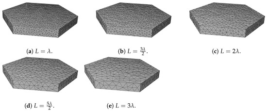
Figure 2.
Examples of different plate geometries with varying maximum edge lengths .
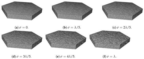
Figure 3.
Examples of different plate geometries with varying roughness amplitudes, .
2.2.1. Particle Orientations
Since DDA computations at this size parameter are time consuming, it is not possible to average over large numbers of particle orientations. Therefore, a compromise is made, whereby the scattering is averaged over a small number of uniformly distributed orientations. The “zyz” rotation convention as described in [22] is used here, which means that the first Euler angle determines the initial rotation about an axis aligned with the incidence direction. In this case, has no effect on the dependence of the scattering and can be set to if only the 1-d scattering is important. Typically, the Euler angles are computed in radians using , and , where X is a number in the range . For hexagonal prism-shaped particles, the range of the and Euler angles can be reduced due to the symmetry of the particle geometry. This allows the orientation averaged scattering to be more quickly approximated compared to a Monte Carlo-based approach. For this rotation convention, with the hexagonal plate initially aligned with the prism axis along the incidence direction, the geometry is symmetric about and repeats every in . The angles are therefore determined by confining X to the range for and for . A diagram showing how the angles and determine the orientation of the plate is shown in Figure 4. The chosen implementation of surface roughness means that the particle is no longer perfectly symmetric in . This falls within ensemble variation, which could be accounted for by additionally averaging over several random realisations of the surface roughness. In this study, it is assumed that the maximum edge length is small enough so that enough mesh elements are present to remove any significant asymmetry without considering ensemble averaging.
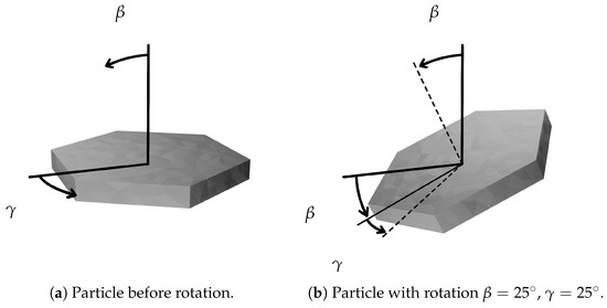
Figure 4.
Diagram showing how the hexagonal plate particle is oriented according to the chosen Euler angles.
In summary, the following limits and values for Euler angles are used to reduce the number of orientations:
- .
- ,, , , , , , , , , , , , , , , .
- ,, , , , , .
2.3. Numerical Methods
Two different numerical methods are used to compute the scattered field from the hexagonal ice plates. These are the discrete dipole approximation (DDA) and the parent beam tracer (PBT) method.
The discrete dipole approximation works by discretising the scatterer into a 3-d array of N total dipoles. Each dipole has a polarisation, and a -dimensional matrix can be constructed to relate the polarisation of one dipole to another. From Maxwell’s equations, a matrix equation can be derived [15]. The matrix equation can then be inverted numerically to arrive at the polarisation of each dipole, from which the scattering properties of the particle can be computed. The DDA method is regarded as a “numerically exact” method, which means that it converges to the true solution with refining discretisation [23]. The accuracy of the DDA method has been well studied, and the error in fulfilment of reciprocity in some tests has been shown to be less than [24]. In this work, the ADDA code is used [25], which recommends as a rule of thumb that the spacing between dipoles d should satisfy . For this study, µm and , so it is chosen that µm. Furthermore, users of the ADDA code are recommended to ensure at least 10 dipoles are present per characteristic length of the particle geometry [26]. Therefore, the minimum value for the maximum edge length is set to so that, in most cases, a sufficient number of dipoles are used to accurately represent the surface roughness. A mesh conversion code which uses a quick sort algorithm is used to construct the dipole arrays for these complex particle geometries [27]. The results from the DDA method here are generally considered the numerical reference data against which the accuracy of the PBT method is measured. The ADDA code is run with numerical solver -iter bcgs2 as described in the ADDA user manual [26].
The PBT method is a recently developed physical–optics hybrid method for large non-spherical particles, including those with surface roughness [28]. It is an approximate method based on the principles of geometric optics (GO), which means it has an accuracy that increases with the size of the particle. To permit the use of GO, the particle must have a size much larger than the wavelength of light. The particle surface is represented as a surface mesh, where each of the facets is grouped according to the macroscopic features of the particle. Each group of facets forms a parent structure, and reflected and refracted beams are produced from the parent structures illuminated by an incident wave. By using Snell’s law and the Fresnel equations of reflection and refraction, the beams can be traced in the near-field to arrive at an approximation for the electric field on the surface of the particle. Then, a surface integral equation [29] can be used to map from the near to the far field. The scattered far field can then be used to compute scattering parameters of interest. The PBT method is one of few physical–optics hybrid methods that can compute the scattered field for particle with physical surface roughnesses. Owing to its basis on GO and a surface integral equation, as opposed to a volume integral equation, it can compute the scattering from large particles within a computation time reduced by several orders of magnitude compared to the DDA method. Nonetheless, it has an accuracy which decreases as the particle becomes more spherical and as the amplitude of the roughness increases. This study provides quantitative results for the range of applicability of the PBT method in the case of hexagonal ice plates with roughness.
3. Results
3.1. Discrete Dipole Approximation
First, the results from the DDA method for variation in roughness are discussed. The phase functions normalised to 1 for and are shown in Figure 5a and Figure 5b, respectively. The reader should refer to Figure 3 for the particle geometries. In general, it can be seen that averaging over the 96 orientations removes most of the fixed-orientation features that might be expected due to specific beam paths. The remaining features include the usual forward scattering peak, a broad halo peak at ∼, and a backscattering peak. Several sharp peaks across the scattering angle range can be seen, which can be attributed to the finite number of chosen angles and an interference effect similar to that observed in thin films. The interference occurs when an externally reflected beam interferes with an internally reflected one as shown in Figure 6a. The angular position of each peak is simply related to by the law of reflection. For example, the first value of corresponds to the first interference peak at . In general, the relative heights of each peak depend on the phase difference between the two beam paths, the Fresnel equations of reflection and transmission, and the projected cross-sectional area. The phase difference is a function of the dimensions of the plate, as well as the wavelength of incident light.
- Close to Direct Forward Scattering: The scattered intensity close to is shown in the upper left inset of the figure. A linear scale is used in the upper left insets here since small fractional differences have a significant effect on the asymmetry parameter. It is found that, at this size parameter, the smooth plate has the strongest forward scattered intensity, while increasing values of result in smaller amplitudes. Interestingly, the data show that scattering by particles with is almost indistinguishable to those with . In summary, the data suggest that surface roughness has almost no effect on the forward scattering if .
- Halo Region: The broad halo peak centred at ∼ can be attributed to the angle of minimum deviation associated with light passing between 2 non-adjacent rectangular facets of the plate [20]. The relative height of this peak, known as the halo ratio, can be defined as . The value of the halo ratio has been proposed as a quantitative measure for identifying the presence of cirrus [30]. Compared to computations with geometric optics (e.g., [9,31]), the halo observed here is broader and relatively weak. The height of this peak can be explained by the large aspect ratio of the plate. More columnar-type ice particles have larger rectangular facets, which in turn leads to a larger fraction of the incident energy being scattered into the halo region. The broadness of the peak is due to the fact that the prism facets have dimensions comparable to the wavelength. This leads to a significant broadening of scattering due to diffractive effects, which cannot be accounted for with classical geometric optics. Similar to the findings of the direct forward scattering, the halo region is almost unaffected by the presence of surface roughness with an amplitude much smaller than the wavelength. The halo peak diminishes as the roughness increases up until , wherein the peak is no longer distinguishable, which agrees with the findings of other studies [32,33,34]. This finding has implications for practical applications which use the halo region as a means of identifying the presence of ice particles. The results show that the absence of a distinguishable halo peak does not necessarily mean that there is an absence of hexagonal ice plates in the sample. Rather, it merely indicates the absence of pristine hexagonal prisms. This agrees with other studies, which have found that classical geometric optics overestimates the intensity of the halo peak [19,35]. Further incorporation of the halo ratio in measuring techniques could provide a useful method of estimating surface roughness and irregularity, especially when combined with the analysis of other experimental evidence, such as scattering pattern symmetry and particle imaging.
- Backscattering: The backscattering in the region – is shown in the upper right insets of Figure 5. Unlike for the forward scattering and halo regions, even small-scale roughness appears to have an effect on the backscattering. As may be expected, the smooth hexagonal plate () shows the strongest backscattering peak. Due to the normalisation of each phase function and the difference in scattering cross sections between datasets, comparing the values at does not provide a very useful insight. Instead, the backscattering ratio is introduced, which is defined here as . The backscattering ratios for increasing values of at are found to be 3.74, 2.86, 1.76, 1.56, 1.41, and 1.42. Increasing the amplitude of surface roughness decreases the backscattering ratio until a value of ∼, where the asymptote appears. Recent studies indicate that two main factors contribute to the backscattering ratio: corner retro-reflection events [36] and coherent backscattering [37]. A retro-reflection can occur when a particle with multiple right-angled facets is illuminated at certain ranges of orientations. Under these conditions, there exist bundles of parallel ray paths which can be shown using geometric optics to scatter into the direct backscattering direction. One possible explanation for the decreasing backscattering ratio is that, as the roughness amplitude increases, the effect of retro-reflection events is reduced, and therefore the backscattering ratio becomes primarily due to coherent backscattering. The effect of coherent backscattering is a well-known wave phenomenon that leads to constructive interference in and close to . The effect can be explained by studying a pair of reciprocal ray paths as shown in Figure 6a. If an incident ray undergoes multiple scattering events and is scattered back along the direction of incidence, then there exists a reciprocal ray which travels along the exact same path but in the opposite direction. This follows as a result of the time-reversal symmetry of Maxwell’s equations. Consequently, the 2 rays travel the same distance and therefore always interfere constructively in the direct backscattering, which leads to a peak in the backscattered intensity. Even without consideration of the phase of the electric field, classical geometric optics often overestimates the backscattering ratio for pristine hexagonal prisms due to the omission of diffraction of outgoing bundles of rays.

Figure 5.
Normalised phase function for hexagonal ice plates with varying amplitudes of surface roughness. Results are computed with the DDA method. Close to direct forward scattering on a linear scale is shown in the upper left inset. The backscattering region is shown in the upper right inset. Parametric sweeps at and are shown in (a,b), with direct comparisons at each roughness amplitude in (c). (a) Maximum edge length . (b) Maximum edge length . (c) Direct comparisons between maximum edge length values and at different roughness amplitudes.


Figure 6.
Important ray paths in scattering by hexagonal ice plates. (a) Plate interference effect, whereby the interference between external reflection and an internally reflected beam path gives rise to the varying peaks across the phase function for orientation averaged hexagonal ice plates. (b) An example of a reciprocal ray pair, which traverse the same path in opposite directions. This example shows a corner retro-reflection, which provides a large contribution to the backscattering of particles with prism [38] geometries.

As increases to values comparable with , the transition region between forward scattering and the halo region is affected, and a secondary maximum in the backscattering (at ) becomes more prominent. The DDA results for variation in the maximum edge length at roughness amplitude are shown in Figure 7. The reader should refer to Figure 2 for the corresponding particle geometries. The DDA results show almost no effect on the orientation averaged scattering due to variation in the maximum edge length. The only discernible differences arise towards the backscattering, when . There are small differences in the shape of the peak at , and the upper right inset of Figure 7 highlights minor differences in the direct backscattering. The backscattering ratios as defined previously for increasing maximum edge length are 2.86, 2.50, 2.74, 2.58, and 2.88. Therefore, it is concluded that changing the maximum edge length has almost no effect on the scattering when the amplitude of roughness is much smaller than the wavelength. By combining the plots in Figure 5a,b, direct comparisons showing the effect of increasing the maximum edge length at different roughness amplitudes can be made. The comparisons are shown in Figure 5c. The upper left and right subplots show that almost identical orientation averaged scattering is predicted by the DDA method for and at each of the maximum edge lengths. The phase function is practically invariant with respect to L for , and even for larger values of , the effect of L can be considered minor. Therefore, it can be said with some certainty that the characterisation of the surface roughness of ice plates can be based solely on the amplitude of the roughness, so long as the amplitude is smaller than the wavelength. Another study found an effective equivalence between surface roughness and irregular geometries by relating the surface tilt angle to a distortion factor [39]. The findings of this work do not fully agree with this equivalence because varying the maximum edge length while keeping the roughness amplitude constant is equivalent to decreasing the surface tilt angles. The results presented here suggest that this should not significantly affect the orientation averaged scattering. Further work is needed to incorporate the resolution of the mesh into the equivalence between the tilt angle and particle distortion. Furthermore, work is needed to determine if the length-scale invariance found in this study can be extended all the way to distorted, smooth geometries.
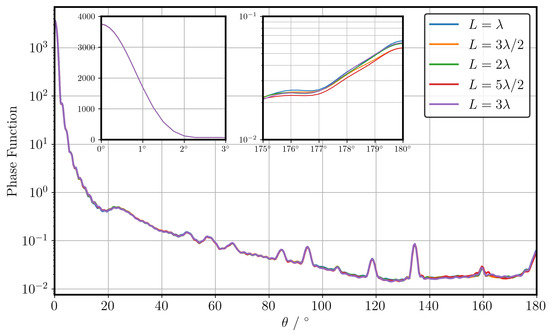
Figure 7.
Normalised phase function for hexagonal ice plates with varying maximum edge length of surface roughness and roughness amplitude . Close to direct forward scattering on a linear scale is shown in the upper left inset. The backscattering region is shown in the upper right inset.
3.2. PBT Results vs. DDA
Second, the results for the PBT against the DDA method for each particle are shown in Figure 8.
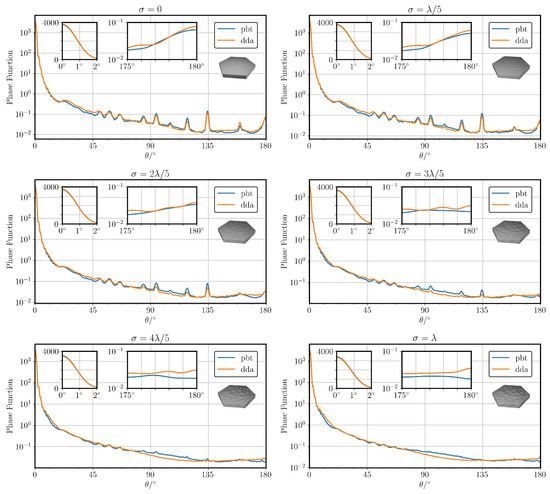
Figure 8.
Comparisons of the normalised phase function for hexagonal ice plates with varying amplitudes of surface roughness and maximum edge length . Close to direct forward scattering on a linear scale is shown in the upper left inset. The backscattering region is shown in the upper centre inset. For reference, each particle is shown as an inset.
Overall, the accuracy of the PBT is best when the particle is smooth and decreases with the amplitude of the roughness. This is to be expected since geometric optics is less accurate in regions where the characteristic length scale is comparable to, or smaller than, the wavelength. It has been pointed out that the geometric optics field is overly sensitive with respect to perturbations in the parameters of the medium [40], which in this case correspond to the fluctuations in the surface topology. For the smooth particle (), the PBT method shows generally good accuracy at all scattering angles. The error in the direct forward () scattering is +1.23% and in the direct backscattering (), it is −18%. One explanation for the underestimation in the backscattering is that this region is highly sensitive to the effects of coherent backscattering. Since the hexagonal plates used here have only a size parameter of 60, the contribution from the edge and corner effects may be significant. The sharp right-angled edges used for the hexagonal plates effectively have an infinitely small radius of curvature. Therefore, traditional GO cannot be expected to capture the physics of field propagation in these regions, and extensions to the geometrical theory of diffraction are needed [41,42]. Of course, it is generally assumed that neglecting such contributions becomes more acceptable with increasing size parameter. For light roughness (), the PBT maintains a reasonable accuracy compared with the DDA. The prediction of the forward scattering peak has an error of −2.57%, the halo region closely resembles the DDA method, and a peak in the direct backscattering is well predicted. Errors in the side scattering (∼) start to become prevalent, which is believed to be a sensitivity of the surface integral method for diffraction and has been recognised in the literature [43]. The PBT accuracy decreases significantly for . For example, as shown in the upper right insets of Figure 8, the DDA predicts a small peak with a backscattering ratio of ∼1.4, but the PBT method shows almost no backscattering peak in this region. Nonetheless, the PBT method shows a promising ability to reproduce the main features of the phase function, even with increasing roughness. The time taken to compute the scattering in each orientation is ∼500 CPU hours for the DDA method, versus ∼1 CPU hour for the PBT method. It should be noted that the relative computational speedup is expected to increase rapidly with the size parameter (the plates were scaled to a volume-equivalent size parameter of 100, but in this case, the DDA method failed to reach convergence).
Next, the PBT results compared with those of the DDA method for variation in maximum edge length for are shown in Figure 9.
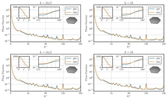
Figure 9.
Comparisons of the normalised phase function for hexagonal ice plates with varying maximum edge lengths of surface roughness with amplitude . Close to the direct forward scattering on a linear scale is shown in the upper left inset. The backscattering region is shown in the upper centre inset. For reference, each particle is shown as an inset. For the case of , the reader is referred to the upper right subplot of Figure 9.
Overall, the agreement between the PBT and the DDA methods is good across all the length scales tested, although the accuracy improves as the maximum edge length increases beyond the wavelength. For smaller values of L, the PBT tends to overestimate side scattering, which can be seen in the upper left of the Figure 9. The computed values for asymmetry parameter g are summarised in Figure 10. The DDA results indicate a weak decrease in the asymmetry parameter with increasing roughness amplitude. The effect of the maximum edge length is small for small roughness amplitudes but becomes more significant as the roughness amplitude becomes comparable to the wavelength. In any case, the surface roughness with scale comparable to the wavelength only appears to affect the asymmetry parameter by, at most, a few %. The figure shows that the PBT method is most accurate for longer maximum edge lengths. Since the DDA method predicts that the scattering is mostly insensitive to the maximum edge length, it can be concluded that the PBT can accurately model surface roughness by setting the maximum edge length to several times the wavelength. Based on these conclusions, it is proposed that the best approach to modelling surface roughness with the PBT method may be to first quantify the amplitude of the roughness, and then second, choose a suitable maximum edge length that is several times larger than the wavelength. Then, based on the finding that the scattering is mostly invariant with respect to the maximum edge length, the PBT method should be a valuable tool capable of predicting various integrated scattering parameters with a relatively small amount of required computations.
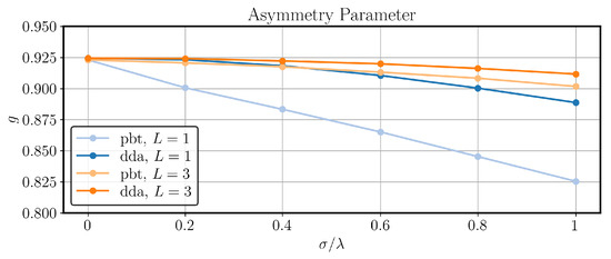
Figure 10.
Comparison of the asymmetry parameter at each maximum edge length and roughness amplitude for the PBT and DDA methods.
The computed values for are summarised in Figure 11. As previously discussed, the DDA method predicts that the variation in the scattering cross section with increasing roughness amplitude is mostly invariant with respect to the maximum edge length. The PBT method shows poor accuracy for a non-smooth surface at but follows the trend of the DDA method at . At , the PBT method is accurate to within ∼.
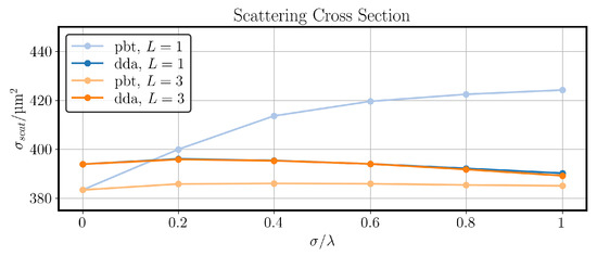
Figure 11.
Comparison of the scattering cross section at each maximum edge length and roughness amplitude for the PBT and DDA methods.
4. Conclusions
Cirrus clouds play a key role in the atmospheric radiation balance. A quantitatively accurate understanding of how ice particles in cirrus interact with incident light is therefore of great importance for predicting and mitigating the effects of climate change. This work aims to help progress this goal by investigating the light scattering properties of hexagonal ice plates with surface roughness at a wavelength µm. The plates have an aspect ratio of 10 and volume-equivalent size parameter of 60. The scattering is averaged over 96 orientations so as to obtain an approximate solution to the orientation-averaged scattering. The DDA method is first used to investigate the effect of roughness on different scattering regions and integrated parameters. Secondly, it is used as a reference to measure the accuracy of the PBT computations. The surface roughness is varied with respect to both a characteristic length scale and a roughness amplitude. The DDA results show that the scattering properties are mostly independent of the roughness length scale, and that roughness has almost no effect on the scattering when the roughness amplitude is much smaller than the wavelength. One exception to this rule is the direct backscattering, which shows a higher degree of sensitivity and decreases with the presence of surface roughness. For the particle geometries studied here, asymmetry parameters decrease by ∼ as the roughness amplitude increases from to . It is found that the scattering from hexagonal ice plates with strong roughness amplitude () does not show a halo peak. This agrees with other studies, and suggests that the halo ratio may not necessarily be enough information to determine that there is an absence of ice particles with hexagonal symmetry. For the PBT, a recently developed, open-source physical–optics hybrid method, the results show the best accuracy for roughness amplitudes in the range and a maximum edge length . In these cases, the asymmetry parameter can be computed to within and the scattering cross section to within ∼.
Author Contributions
Conceptualisation, H.B. and E.H.; methodology, H.B.; software, H.B.; validation, H.B.; formal analysis, H.B.; investigation, H.B.; resources, H.B.; data curation, H.B.; writing—original draft preparation, H.B.; writing—review and editing, H.B and E.H.; visualisation, H.B.; supervision, E.H.; project administration, E.H.; funding acquisition, E.H. All authors have read and agreed to the published version of the manuscript.
Funding
This research was funded by the Natural Environment Research Council (NERC), United Kingdom, grant NE/T00147X/1.
Institutional Review Board Statement
Not applicable.
Informed Consent Statement
Not applicable.
Data Availability Statement
The raw data supporting the conclusions of this article will be made available by the authors on request. The data are not publicly available due to privacy.
Conflicts of Interest
The authors declare no conflicts of interest. The funders had no role in the design of the study; in the collection, analyses, or interpretation of data; in the writing of the manuscript; or in the decision to publish the results.
Abbreviations
The following abbreviations are used in this manuscript:
| DDA | Discrete Dipole Approximation |
| PBT | Parent Beam Tracer |
References
- Baran, A.J. A review of the light scattering properties of cirrus. J. Quant. Spectrosc. Radiat. Transf. 2009, 110, 1239–1260. [Google Scholar] [CrossRef]
- Mishchenko, M.I.; Hovenier, J.W.; Travis, L.D. Light Scattering by Nonspherical Particles; Academic Press: Cambridge, MA, USA, 1999. [Google Scholar]
- Hahn, C.J.; Warren, S.G. A Gridded Climatology of Clouds over Land (1971–96) and Ocean (1954–97) from Surface Observations Worldwide; Oak Ridge National Laboratory, Carbon Dioxide Information Analysis Center: Oak Ridge, TN, USA, 2007. [Google Scholar] [CrossRef]
- Mitchell, C.J.; Porco, C.C.; Weiss, J.W. Tracking the Geysers of Enceladus into Saturn’s E Ring. Astron. J. 2015, 149, 156. [Google Scholar] [CrossRef]
- Martin, W.; Baross, J.; Kelley, D.; Russell, M.J. Hydrothermal vents and the origin of life. Nat. Rev. Microbiol. 2008, 6, 805–814. [Google Scholar] [CrossRef] [PubMed]
- Morello, C.; Berg, M.J. A light scattering analysis of the cryovolcano plumes on enceladus. J. Quant. Spectrosc. Radiat. Transf. 2024, 322, 109018. [Google Scholar] [CrossRef]
- Heymsfield, A.J.; Krämer, M.; Luebke, A.; Brown, P.; Cziczo, D.J.; Franklin, C.; Lawson, P.; Lohmann, U.; McFarquhar, G.; Ulanowski, Z.; et al. Cirrus Clouds. Meteorol. Monogr. 2017, 58, 2.1–2.26. [Google Scholar] [CrossRef]
- Peltoniemi, J.I.; Lumme, K.; Muinonen, K.; Irvine, W.M. Scattering of light by stochastically rough particles. Appl. Opt. 1989, 28, 4088–4095. [Google Scholar] [CrossRef]
- Macke, A.; Mueller, J.; Raschke, E. Single Scattering Properties of Atmospheric Ice Crystals. J. Atmos. Sci. 1996, 53, 2813–2825. [Google Scholar] [CrossRef]
- Muinonen, K. Light Scattering by Gaussian Random Particles. Earth Moon Planets 1996, 72, 339–342. [Google Scholar] [CrossRef]
- Mishchenko, M.I. Calculation of the amplitude matrix for a nonspherical particle in a fixed orientation. Appl. Opt. 2000, 39, 1026–1031. [Google Scholar] [CrossRef]
- Muinonen, K.; Nousiainen, T.; Lindqvist, H.; Munoz, O.; Videen, G. Light scattering by Gaussian particles with internal inclusions and roughened surfaces using ray optics. J. Quant. Spectrosc. Radiat. Transf. 2009, 110, 1628–1639. [Google Scholar] [CrossRef]
- Collier, C.; Hesse, E.; Taylor, L.; Ulanowski, Z.; Penttilä, A.; Nousiainen, T. Effects of surface roughness with two scales on light scattering by hexagonal ice crystals large compared to the wavelength: DDA results. J. Quant. Spectrosc. Radiat. Transf. 2016, 182, 225–239. [Google Scholar] [CrossRef]
- Riskilä, E.; Lindqvist, H.; Muinonen, K. Light scattering by fractal roughness elements on ice crystal surfaces. J. Quant. Spectrosc. Radiat. Transf. 2021, 267, 107561. [Google Scholar] [CrossRef]
- Purcell, E.M.; Pennypacker, C.R. Scattering and adsorption of light by nonspherical dielectric grains. Astrophys. J. 1973, 186, 705–714. [Google Scholar] [CrossRef]
- Waterman, P. Matrix formulation of electromagnetic scattering. Proc. IEEE 1965, 53, 805–812. [Google Scholar] [CrossRef]
- Liu, Q.H. The PSTD algorithm: A time-domain method requiring only two cells per wavelength. Microw. Opt. Technol. Lett. 1997, 15, 158–165. [Google Scholar] [CrossRef]
- Grynko, Y.; Shkuratov, Y.; Förstner, J. Light scattering by irregular particles much larger than the wavelength with wavelength-scale surface roughness. Opt. Lett. 2016, 41, 3491–3494. [Google Scholar] [CrossRef]
- Neshyba, S.P.; Lowen, B.; Benning, M.; Lawson, A.; Rowe, P.M. Roughness metrics of prismatic facets of ice. J. Geophys. Res. Atmos. 2013, 118, 3309–3318. [Google Scholar] [CrossRef]
- Bohren, C.F.; Huffman, D.R. Absorption and Scattering of Light by Small Particles; John Wiley & Sons: Hoboken, NJ, USA, 1983. [Google Scholar]
- Shewchuk, J.R. Triangle: Engineering a 2D quality mesh generator and Delaunay triangulator. In Proceedings of the Applied Computational Geometry Towards Geometric Engineering, Philadelphia, PA, USA, 27–28 May 1996; Lin, M.C., Manocha, D., Eds.; Springer: Berlin/Heidelberg, Germany, 1996; pp. 203–222. [Google Scholar]
- Muinonen, K.; Nousiainen, T.; Fast, P.; Lumme, K.; Peltoniemi, J. Light scattering by Gaussian random particles: Ray optics approximation. J. Quant. Spectrosc. Radiat. Transf. 1996, 55, 577–601. [Google Scholar] [CrossRef]
- Yurkin, M.A. Chapter 9-Discrete dipole approximation. In Light, Plasmonics and Particles; Mengüç, M.P., Francoeur, M., Eds.; Nanophotonics; Elsevier: Amsterdam, Netherlands, 2023; pp. 167–198. [Google Scholar] [CrossRef]
- Schmidt, K.; Yurkin, M.A.; Kahnert, M. A case study on the reciprocity in light scattering computations. Opt. Express 2012, 20, 23253–23274. [Google Scholar] [CrossRef]
- Yurkin, M.A.; Hoekstra, A.G. The discrete-dipole-approximation code ADDA: Capabilities and known limitations. J. Quant. Spectrosc. Radiat. Transf. 2011, 112, 2234–2247. [Google Scholar] [CrossRef]
- Yurkin, M.A. User Manual for the Discrete Dipole Approximation Code ADDA 1.4.0. 2020. Available online: https://github.com/adda-team/adda/blob/master/doc/manual.pdf (accessed on 4 April 2023).
- Penttilä, A. Fortran 95 Implementation of Meshconvert Computer Code. 2023. Available online: https://wiki.helsinki.fi/xwiki/bin/view/PSR/Planetary%20System%20Research%20group/People/Antti%20Penttil%C3%A4/Collection%20of%20codes/ (accessed on 12 July 2023).
- Ballington, H.; Hesse, E. A light scattering model for large particles with surface roughness. J. Quant. Spectrosc. Radiat. Transf. 2024, 323, 109054. [Google Scholar] [CrossRef]
- Karczewski, B.; Wolf, E. Comparison of Three Theories of Electromagnetic Diffraction at an Aperture.* Part I: Coherence Matrices. J. Opt. Soc. Am. 1966, 56, 1207–1214. [Google Scholar] [CrossRef]
- Dandini, P.; Ulanowski, Z.; Campbell, D.; Kaye, R. Halo ratio from ground-based all-sky imaging. Atmos. Meas. Tech. 2019, 12, 1295–1309. [Google Scholar] [CrossRef]
- Baran, A.J. From the single-scattering properties of ice crystals to climate prediction: A way forward. Atmos. Res. 2012, 112, 45–69. [Google Scholar] [CrossRef]
- Yang, P.; Liou, K.N. Single-scattering properties of complex ice crystals in terrestrial atmosphere. Contrib. Atmos. Phys. 1998, 71, 223–248. [Google Scholar]
- Mishchenko, M.I.; Macke, A. How big should hexagonal ice crystals be to produce halos? Appl. Opt. 1999, 38, 1626–1629. [Google Scholar] [CrossRef]
- Ulanowski, Z. Ice analog halos. Appl. Opt. 2005, 44, 5754–5758. [Google Scholar] [CrossRef]
- Hesse, E.; Ulanowski, Z. Scattering from long prisms computed using ray tracing combined with diffraction on facets. J. Quant. Spectrosc. Radiat. Transf. 2003, 79–80, 721–732. [Google Scholar] [CrossRef]
- Borovoi, A.G.; Grishin, I.A. Scattering matrices for large ice crystal particles. J. Opt. Soc. Am. A 2003, 20, 2071–2080. [Google Scholar] [CrossRef]
- Muinonen, K.; Lumme, K.; Peltoniemi, J.; Irvine, W.M. Light scattering by randomly oriented crystals. Appl. Opt. 1989, 28, 3051–3060. [Google Scholar] [CrossRef]
- Grünbaum, B. Isogonal Prismatoids. Discret. Comput. Geom. 1997, 18, 13–52. [Google Scholar] [CrossRef][Green Version]
- Liu, C.; Panetta, R.L.; Yang, P. The effective equivalence of geometric irregularity and surface roughness in determining particle single-scattering properties. Opt. Express 2014, 22, 23620–23627. [Google Scholar] [CrossRef] [PubMed]
- Kravtsov, Y.; Orlov, Y. Geometrical Optics of Inhomogeneous Media; Springer Series on Wave Phenomena; Springer: Berlin/Heidelberg, Germany, 2011. [Google Scholar]
- Borovoi, A.G. Light scattering by large particles: Physical optics and the shadow-forming field. In Light Scattering Reviews 8: Radiative Transfer and Light Scattering; Springer: Berlin/Heidelberg, Germany, 2013; pp. 115–138. [Google Scholar] [CrossRef]
- Keller, J.B. Geometrical theory of diffraction. J. Opt. Soc. Am. 1962, 52, 116–130. [Google Scholar] [CrossRef] [PubMed]
- Bi, L.; Yang, P.; Kattawar, G.W.; Hu, Y.; Baum, B.A. Diffraction and external reflection by dielectric faceted particles. J. Quant. Spectrosc. Radiat. Transf. 2011, 112, 163–173. [Google Scholar] [CrossRef]


Disclaimer/Publisher’s Note: The statements, opinions and data contained in all publications are solely those of the individual author(s) and contributor(s) and not of MDPI and/or the editor(s). MDPI and/or the editor(s) disclaim responsibility for any injury to people or property resulting from any ideas, methods, instructions or products referred to in the content. |
© 2024 by the authors. Licensee MDPI, Basel, Switzerland. This article is an open access article distributed under the terms and conditions of the Creative Commons Attribution (CC BY) license (https://creativecommons.org/licenses/by/4.0/).