Abstract
This study is an additional investigation of stratosphere–troposphere coupling based on the recent stratospheric winter descriptions in five distinct modes: January, February, Double, Dynamical, and Radiative. These modes, established in a previous study, categorize the main stratospheric winter typologies modulated by the timing of important sudden stratospheric warmings (SSWs) and final stratospheric warmings (FSWs). The novelty of this research is to investigate the Northern Annular Mode, mean sea level pressure (MSLP) anomalies in the Ural and Aleutian regions, and the decomposition of Eliassen–Palm flux into wavenumbers 1 and 2 within each mode. The results show that the January and Double modes exhibit similar pre-warming surface signals, characterized by Ural blocking and Aleutian trough events preceding weak polar vortex events. The January mode displays a positive MSLP anomaly of +395 Pa (−191 Pa) in the Ural (Aleutian) region in December, while the Double mode shows +311 Pa (−89 Pa) in November. These modes are primarily wave-1 driven, generating tropospheric responses via negative Arctic Oscillation patterns. Conversely, the February and Dynamical modes show opposite signals, with Aleutian blocking and Ural trough events preceding strong polar vortex events. In December, the February mode exhibits MSLP anomalies of +119 Pa (Aleutian) and −180 Pa (Ural), while the Dynamical mode shows +77 Pa and −184 Pa, respectively. These modes, along with important SSWs in February and dynamical FSWs, are driven by both wave-1 and wave-2 and do not significantly impact the troposphere. The Radiative mode’s occurrence is strongly related to the Aleutian blocking presence. These findings confirm that SSW timing is influenced by specific dynamical forcing related to surface precursors and underscore its importance in subsequent tropospheric responses. This study establishes a connection between early winter tropospheric conditions and upcoming stratospheric states, potentially improving seasonal forecasts in the northern hemisphere.
1. Introduction
The understanding of stratosphere–troposphere coupling is a crucial aspect of improving seasonal weather predictions in atmospheric sciences [1,2]. This field of research has gained significant attention due to the recognized mutual influence between the stratospheric polar vortex and the tropospheric circulation during the northern hemisphere winter [3]. One of the key models, developed by Matsuno [4], explains that variations in the strength of the wintertime stratospheric circulation are a result of the interaction between the mean flow and upward propagating planetary waves that transport westward momentum from the troposphere. These interactions can give rise to sudden stratospheric warming (SSW) events, characterized by increased polar cap temperatures, weakened polar vortex, and even the reversal of westerly winds in extreme cases [5]. The subsequent stratospheric circulation anomalies can descend into the troposphere, influencing surface weather patterns over several weeks [3,6].
The northern hemisphere annular mode (NAM) is a commonly used measure for assessing stratosphere–troposphere coupling during SSW events [7]. Baldwin and Dunkerton [6], for example, computed NAM indices from weak and strong vortex composites and observed that these events are often followed by negative and positive phases, respectively, of the Arctic Oscillation (AO) pattern at the surface, which can persist for up to two months. The stratospheric anomaly propagating downward has numerous consequences for tropospheric weather, including shifts in storm track locations, changes in the likelihood and intensity of mid-latitude storms, variations in the frequency of high-latitude blocking events, and the occurrence of cold air outbreaks across the hemisphere [8]. However, it is worth noting that not all SSW events result in a systematic tropospheric response [1], and the same is true for final stratospheric warming (FSW) events [9]. Therefore, there has been ongoing research in the scientific community to classify SSW and FSW events and understand the factors that determine their different impacts on tropospheric circulation.
Traditionally, extreme SSW events have been classified as “major” based on the reversal of westerly winds at 10 hPa–60° N [10]. However, even though it is a relevant metric for detecting a perturbed polar vortex [11], this criterion alone does not indicate whether the stratospheric anomaly propagates downward. Other studies have classified SSW events based on the geometry of the polar vortex, distinguishing between displaced and splitting types [12,13,14,15]. Although Mitchell et al. [15] found that splitting types tend to propagate downward compared to displacement types, aligning with the upward fluxes of wavenumbers 1 and 2 observed by Nakagawa and Yamazaki [16], this statistical difference was not consistently replicated by Charlton and Polvani [12] and Lehtonen and Karpechko [17]. This inconsistency was also reported in Maycock and Hitchcock [18], confirming that the polar vortex geometry is not an optimal predictor of tropospheric impacts following SSWs. It is similar for the wave geometry criterion, as downward impacts can occur after both displacement and splitting SSW events, as seen in the SSWs of January 2009 (split) and January 2010 (displaced) [19,20].
The role of tropospheric blocking events in the pre- and post-warming phases has also been investigated in many studies, demonstrating the importance of the Euro-Atlantic and Pacific regions regarding the propagation of wavenumbers 1 and 2 [21,22,23]. Also, certain blocking regions such as the Ural in November seemed to exhibit stronger subsequent tropospheric responses with negative AO-like patterns in December and January [24,25].
Some studies have directly classified SSWs based on their tropospheric responses, such as absorbing or reflecting types [26], the persistence of stratospheric anomalies [27,28], or surface observations of the North Atlantic Oscillation [29] and North Atlantic storm track response [30]. Thus, these different studies highlight the difficulty in finding the most robust criteria responsible for the tropospheric responses occurring after SSWs. Nevertheless, even though the mechanism responsible for the descending effect is still unclear, the persistence of anomalies in the lower stratosphere seems to play a crucial role in this process [28,31,32].
On the other hand, FSW events have been classified based on their timing and nature, distinguishing between “early” and “dynamical” or “late” and “radiative” events [33,34]. The mechanism underlying mid-SSWs and early dynamical FSWs, both driven by waves, is similar [35]. In addition to its effects on transport and the mixing of stratospheric ozone [9,33], the timing of the FSW can exert an influence on the tropospheric circulation and the sea ice thickness through autumn [36].
Recently, Mariaccia et al. [37] (hereafter M22) proposed a new classification based on empirical orthogonal functions of stratospheric zonal wind fluctuation patterns at the edge of the polar vortex. Their study suggests the existence of four scenarios followed by the northern hemisphere winter stratosphere, influenced by the timing of SSWs and FSWs. Three of them are modulated by the timings of important SSW events, lumping all SSW events for which the zonal mean zonal wind at 10 hPa–60° N drops below 10 m · s−1 in mid-wintertime. The benefit of this criterion is that it considers not only major SSWs but also the warming events that significantly weaken the polar vortex without reversing the wind [38]. The last scenario represents winters without important SSWs but differing in the timing of FSW (dynamical and early or radiative and late).
Interestingly, Monnin et al. [39] conducted research on the impact of SSW timing on tropospheric responses in Europe. The findings indicate that SSWs occurring in December and January have a more significant surface impact compared to SSWs in February and March. Focusing on the intra-seasonal variability of anomalous wave activity, Díaz-Durán et al. [40] showed that weak and strong polar vortex events in early winter present an enhancement and inhibition of wavenumber 1 wave (wave-1) activity, respectively, while mid- and late-winter weak vortex events exhibit an enhancement of wave-1 and wave-2. Therefore, these recent studies provide strong motivation for investigating the teleconnection between the stratosphere and troposphere during winter months using the classification established in M22.
The primary aim of this study is to provide a new perspective on the coupling between the stratosphere and troposphere in the northern hemisphere utilizing the classification scheme reported in M22, which underscores the importance of the timing of important SSW. To achieve this, we will first analyze the descent of stratospheric anomalies into the troposphere within each scenario by examining their mean Northern Annular Mode (NAM) evolution. Subsequently, we will investigate the surface impacts and the existence of any surface precursors through the examination of mean sea level pressure (MSLP) anomalies in the Ural and Aleutian regions. Finally, we will seek to gain a more comprehensive understanding of the underlying dynamical processes within each scenario by assessing the propagation direction of wave-1 and wave-2 and their interaction with the mean flow through the Eliassen–Palm (EP) flux.
2. Data and Methods
2.1. ERA5 Reanalysis
Since 2016, the European Centre for Medium-Range Weather Forecasts (ECMWF) has been generating a state-of-the-art reanalysis dataset called ERA5. A technical description of the ERA5 reanalysis can be found in Hersbach et al. [41]. Initially covering the period from 1950 to the present, the ERA5 reanalysis benefited in 2023 from a further extension back to 1940, offering the most extended time series of reanalysis available. However, as this study is based on the classification established for the winters from 1950 to 2020, this last available decade is not exploited here.
According to Bell et al. [42], the ERA5 reanalysis possesses an accurate depiction of the SSW in 1952, confirming its fidelity in the pre-satellite era. Furthermore, recent studies have demonstrated that ERA5 temperature reanalysis accurately reproduces observed temperatures and their variability within the upper stratosphere during winter [43,44]. Therefore, the ERA5 data set is particularly appropriate for studying stratosphere–troposphere coupling over decades, specifically during the winter season.
The ERA5 data are available at 37 pressure levels, covering the entire troposphere–stratosphere region from 1000 to 1 hPa, with 11 levels between 100 and 1 hPa. For our analysis, we extracted the daily variables required to compute the Northern Annular Mode (NAM) indices and Eliassen–Palm flux from the ERA5 reanalysis data at these pressure levels. Our analysis covers a 2.5° × 2.5° grid from 20° N poleward and spans from 1950 to 2020, encompassing a total of 70 winters. To evaluate the surface signals of each composite, the monthly means of the mean sea level pressure (MSLP) were extracted from 40° N poleward over the studied period. The winter season in our analysis starts on November 1st and concludes on May 1st, spanning a period of 182 days.
2.2. Classification of Winters in M22
In Mariaccia et al. [37], winters were classified based on the evolution of the anomaly of stratospheric zonal mean zonal winds at the edge of the polar vortex using the ERA5 reanalysis data. First, an empirical orthogonal function (EOF) analysis was performed on the zonal wind anomalies of the 70 winters between 1950 and 2020 to identify the main patterns of variability. The first three EOF modes explained 65.3% of the variance: the January mode (EOF1, 31.7%), the February mode (EOF2, 22.2%), and the Double mode (EOF3, 11.4%). The names correspond to their timing of occurrence for the January and February modes and to the presence of two SSWs (one in December and another one in February/March)over the same winter for the Double mode.
Winters with important SSWs were then selected if zonal winds at 60° N and 10 hPa dropped below 10 m·s−1 at least once between 15 December and 1 March, resulting in 50 qualifying winters. Each winter’s wind anomalies were decomposed into the three EOF modes, with the highest coefficient indicating the primary scenario for that winter, provided the coefficient exceeded a threshold of 0.2. This process classified 41 out of 50 winters into the January (17 winters), February (17 winters), or Double modes (7 winters), while the remaining 9 winters did not fit any single scenario precisely.
The 20 winters without mid-winter important SSW events were further analyzed based on the timing of their final stratospheric warmings (FSWs) and classified into the radiative final warming (Radiative) mode (5 winters) or dynamical final warming (Dynamical) mode (15 winters), following Butler and Domeisen [9]. The complete list of winters associated with each scenario can be found in Appendix A.
2.3. Calculating the NAM Indices
The Northern Annular Mode (NAM), also known as the Arctic Oscillation (AO), is a key measure of dynamic variability over the hemispheric scale during the winter season. It is computed by determining the leading EOF that captures the dominant patterns of variability from 20° N poleward. The computation of NAM indices enables us to assess the influence of stratospheric variability on the spatial patterns observed in the troposphere.
Several methods exist for computing NAM indices, including surface-based EOFs, height-dependent EOFs, and zonal-mean EOFs. Each method has its advantages and drawbacks. The first two methods have limitations in capturing realistic annular variability in the middle atmosphere, as well as computational costs. In contrast, the zonal-mean EOFs method, as described by Baldwin and Thompson [7], based on daily averaged, zonally averaged, year-round geopotential height, consistently captures annular variability structures and is employed in this study.
Thus, we computed NAM indices for the 70 winters spanning from 1950 to 2020. Subsequently, we averaged the daily NAM indices over the winters associated with each mode to obtain the mean time-height development of the northern annular mode. By applying this approach, we can analyze the behavior of the NAM and its link to stratospheric variability, providing valuable insights into the stratosphere–troposphere coupling over the winter season.
2.4. Statistical Significance Assessment: Wilcoxon Signed-Rank Test
To assess the significance of the anomalies in the NAM evolutions and MSLP anomalies, we employed the Wilcoxon signed-rank test [45]. This non-parametric test was chosen for its robustness and suitability for comparing paired data samples that may not follow a normal distribution. The Wilcoxon signed-rank test evaluates whether the median of the differences between paired observations is zero, which is ideal for our dataset, where anomalies may not adhere to normality assumptions. This rigorous statistical validation ensures that our identified anomalies are robust and reliable indicators of the atmospheric patterns under investigation.
2.5. Ural and Aleutian Blocking Regions
The Ural and Aleutian regions are well-documented as significant markers of tropospheric wave forcing, which can trigger SSW events that may subsequently impact these regions (e.g., [21,24,25,40,46]). Here, the connection between these regions and the different modes is investigated; firstly, in November and December based on the monthly mean MSLP anomaly to assess whether they act as precursors of the coming stratosphere or not. Then, the lead–lag correlation coefficients are computed between the Ural and Aleutian blocking indices with the different modes to more deeply investigate their connections; in particular, when the stratosphere leads the troposphere. These regions are defined according to the examination of the regression of 45 to 80° N meridional mean MSLP onto the 10 hPa NAM performed by Kohler et al. [25] with the ERA5 data.
2.6. The Eliassen–Palm Flux
The Eliassen–Palm (EP) flux is a vector that characterizes the direction of small amplitude atmospheric waves as well as the magnitude of eddy heat flux and momentum flux [47]. It serves as a valuable diagnostic tool for investigating wave-mean flow interactions, and, consequently, the coupling between the stratosphere and troposphere [48]. The divergence of the EP flux provides information about the acceleration or deceleration of the zonal mean zonal wind.
In this study, ERA5 data were extracted based on pressure levels and latitude degrees, and the divergence of the EP flux was computed using the methodology described by Jucker [49]. This approach accounts for spherical geometry, the aspect ratio of the figures, and the units of the vector components. The components of the EP flux in pressure coordinates are calculated using the equations introduced by Andrews et al. [50] and are then decomposed into wavenumber 1 (hereafter wave-1) and wavenumber 2 (hereafter wave-2).
3. Results
3.1. Northern Annular Mode Indices: Stratosphere–Troposphere Coupling
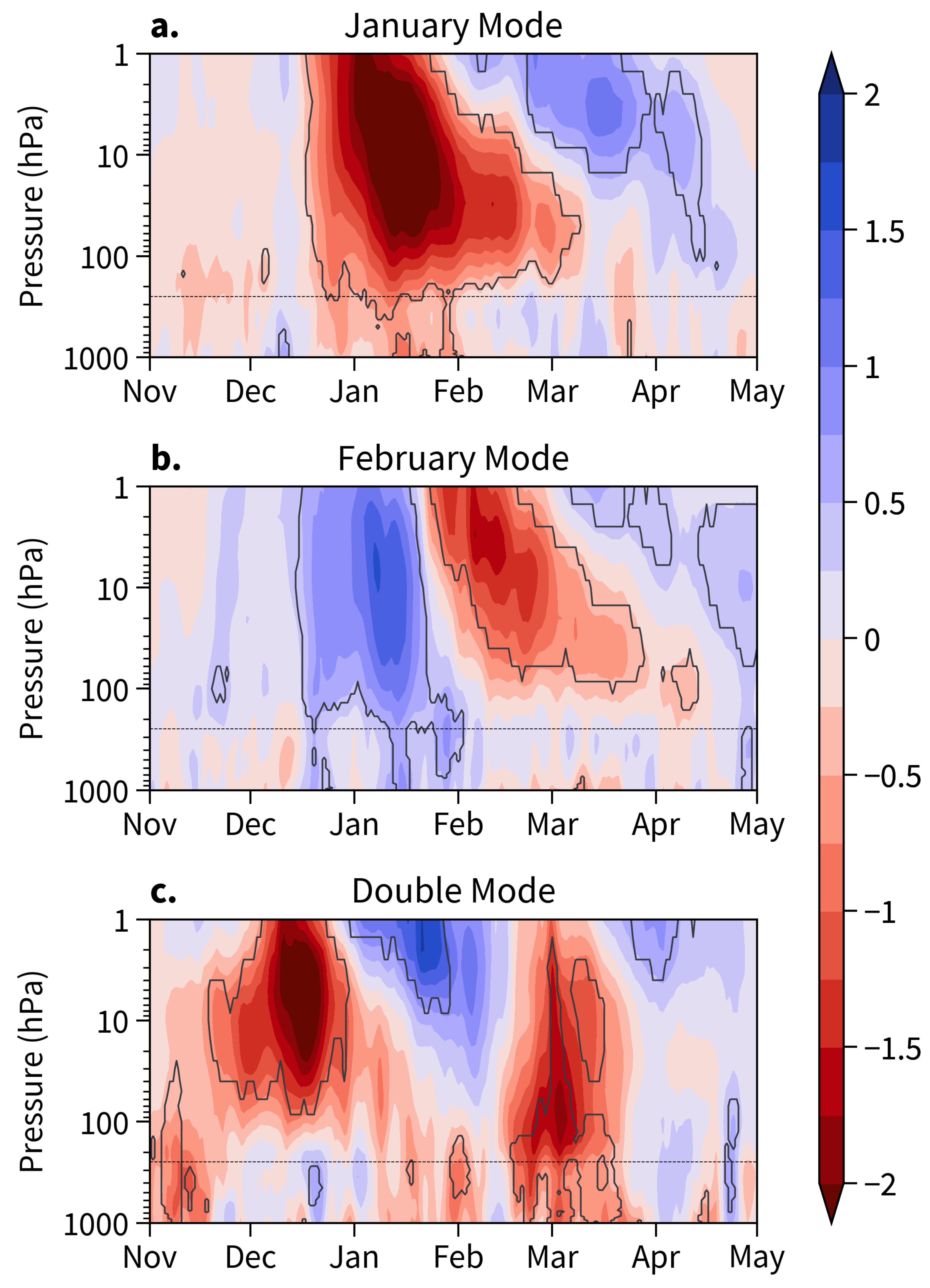
Figure 1 and Figure 2 illustrate the daily average of the time–height development of the NAM indices in both the troposphere and stratosphere for the five modes: January, February, Double, Dynamical, and Radiative modes. Weak and warm polar vortex periods are represented in red, while strong and cold periods are shown in blue. The figure includes solid black contour lines to highlight significant anomalies identified based on the Wilcoxon signed-rank test. Since the analysis is performed on averaged result smoothing signals, the presented evolutions do not represent exactly how the winters unfold. This is why only the significant signals according to the Wilcoxon’s t-test will be discussed here and in the rest of this paper. The delimitation between the troposphere and the stratosphere is indicated at 250 hPa, reported to be the approximate pressure level of the tropopause [51].
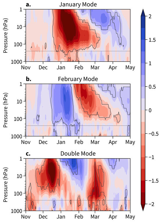
Figure 1.
Mean time–height development of the northern annular mode indices for the winters associated with the perturbed modes: the January mode (a), the February mode (b), and the Double mode (c). The indices have a daily resolution and are non-dimensional. Negative values (red) correspond to a weak polar vortex, and positive values (blue) correspond to a strong polar vortex. The black lines contour areas with statistical confidence at the 95% level according to a Wilcoxon signed-rank test. The horizontal black dashed lines indicate the approximate delimitation between the troposphere and the stratosphere.

Figure 2.
Mean time–height development of the northern annular mode indices for the winters associated with the unperturbed modes: the Dynamical mode (a) and the Radiative mode (b). The indices have a daily resolution and are non-dimensional. Negative values (red) correspond to a weak polar vortex, and positive values (blue) correspond to a strong polar vortex. The black lines contour areas with statistical confidence at the 95% level according to a Wilcoxon signed-rank test. The horizontal black dashed lines indicate the approximate delimitation between the troposphere and the stratosphere.
Overall, these NAM evolutions are consistent with prior research, which has established that stratospheric anomalies exhibit longer timescales compared to tropospheric fluctuations. Furthermore, anomalies often manifest initially in the upper stratosphere before descending downward [6,15]. Anomalies reaching the lower stratosphere tend to have extended durations, attributable to the longer radiative time scale. Strong anomalies located just above the tropopause demonstrate a greater likelihood of downward propagation into the troposphere, underscoring the significance of this factor [31]. Most importantly, these NAM evolutions show that these different modes have, on average, distinct stratosphere–troposphere teleconnections throughout the winter. One aspect of particular interest among the modes is whether the stratospheric anomalies descend into the troposphere, whether generated by important SSW, FSW, or strong vortex events.
Regarding the January mode (see Figure 1a), towards the end of December, all stratospheric levels experience a simultaneous emergence of a significant positive anomaly associated with weak vortex events caused by an important SSW. This phenomenon rapidly propagates throughout the stratosphere, with a high significance between December and January, suggesting a potential wave resonance due to barotropic mode excitation [52]. It extends across the entire stratosphere and subsequently descends into the troposphere, notably reaching the Earth’s surface in January. In February, a positive anomaly descends from the upper to lower stratosphere, with a slight rise at the tropopause, which halts its propagation into the troposphere. The FSW, typically occurring around 20 April [37], does not generate an intense signal in either the stratosphere or the troposphere. These results conform to the expected winter patterns associated with this scenario, including the occurrence of important SSWs in mid-January, followed by a minor strengthening of the polar vortex in March, concluding in April. It is worth noting that the initial positive and negative irregularities observable in early December above the tropopause and on the surface, respectively, may suggest early indications of the forthcoming important SSW occurrence.
In the case of the February mode (see Figure 1b), a noticeable negative anomaly is observed in the latter half of November, just above the tropopause, and it persists for a few days. It is important to note that the February mode exhibits a different starting pattern than the January mode in the lower stratosphere. Subsequently, a significant negative anomaly, signaling the occurrence of a strong vortex event, emerges and covers the entire stratosphere from mid-December to the end of January. As this anomaly descends toward the tropopause, it begins to significantly impact the troposphere, reaffirming the crucial role of this factor once again [28,31]. Following this, a positive anomaly primarily appears in the upper stratosphere at the end of January, with a descending phase that extends into the lower stratosphere, lasting until April. However, there is no significant descent into the troposphere compared to what it is observed in the January mode, even though a small significant negative NAM signal is found at the surface in March. This suggests that winters with SSWs in February propagate downward but possess very different anomaly descents in the following months. Finally, from March onward, a weak negative anomaly signal develops in the upper stratosphere, indicating the final formation of the polar vortex with weak winds before the occurrence of the FSW, which is often characterized by late and radiative events [37].
Winters associated with the Double mode (see Figure 1c) exhibit, on average, a positive anomaly in the troposphere from mid-November. Surprisingly, unlike the January and February modes, this anomaly appears to propagate upward from the surface and precedes another positive anomaly covering the entire stratosphere from mid-December, corresponding to the first important SSW’s occurrence. This upward propagation suggests that the positive anomaly at the surface acts as a tropospheric precursor to the subsequent important SSW’s appearance. Hence, this anomaly propagation exemplifies the bidirectional stratospheric–tropospheric dynamical coupling and its potential usefulness for seasonal-scale climate forecasts. The positive anomaly descends into the lower stratosphere and propagates into the troposphere from mid-January. Concurrently, a negative anomaly emerges in the upper stratosphere from the beginning of January, indicating the reformation of the polar vortex. Starting from mid-February, a new positive anomaly corresponding to the second important SSW’s occurrence emerges, covering both the stratosphere and troposphere until the end of March. As a result, the Double mode exhibits a very special stratosphere–troposphere coupling with two important SSWs propagating into the troposphere.
As a first conclusion, it appears that important SSWs occurring in the January and Double modes extend clearly in the troposphere compared to those in the February mode. This likely results from weaker and more disparate downward propagations among winters in the February mode. However, even though the initial surface weather regime also contributes to the upcoming surface patterns [17] , the surface signal arising in March may represent evidence of this delayed downward propagation following important SSWs. From this perspective, these outcomes align with the findings of Monnin et al. [39], who found that early-winter (December/January) SSW events do not propagate further downward than late-winter SSWs (February/March). Nonetheless, according to NAM evolutions, winters in the February mode tend to propagate less abruptly into the troposphere than those in the January mode.
In line with their zonal wind evolutions, both sub-modes exhibit a negative anomaly in the stratosphere, indicative of a persistent polar vortex that extends until the end of winter, finishing with either dynamical or radiative FSWs.
For the Dynamical mode (Figure 2a), a negative anomaly forms on average in the stratosphere in December. This negative anomaly propagates downward, gradually encompassing the entire stratosphere while intensifying until the end of February, at which point it initiates descent towards the troposphere. Consequently, the negative anomalies reach the Earth’s surface until the end of March. Interestingly, in early March, a positive anomaly appears at the top of the diagram, which corresponds to the occurrence of a dynamical FSW. This latter one disrupts the polar vortex, resembling the important SSWs observed in the three perturbed modes, but with less intensity. Throughout March, this tilted positive anomaly propagates downward but does not significantly penetrate into the troposphere.
Lastly, regarding the Radiative mode (Figure 2b), in December, a positive anomaly descends while gaining strength, reaching the tropopause region and influencing the troposphere. Concurrently, a robust negative anomaly begins to form in the upper stratosphere. This negative anomaly propagates downward, covering the entire stratosphere from mid-January to mid-April while maintaining its intensity, indicating a persistently strong vortex throughout winter. From January to April, the tropospheric surface experiences the effects of this robust polar vortex. As expected, it presents some interesting sharp time-lag differences from the Dynamical mode in late winter.
In the next section, we will explore the surface regions affected in the Northern Hemisphere over the course of these five modes. This investigation aims to identify potential precursors, particularly those located in the Ural and Aleutian regions, and then to assess the impact on the surface following important SSWs, FSWs, and strong vortex events.
3.2. MSLP Anomalies and Regional Blocking
3.2.1. Monthly MSLP Anomalies for Stratospheric Modes
Figure 3 illustrates the evolution of monthly mean MSLP anomalies for the five modes from November to March. The stippled areas indicate the regions of highest significance according to the Wilcoxon signed-rank test. Only the stippled anomalies will be described here to focus only on significant signals. Table 1 indicates the mean values of the MSLP anomaly computed in the Ural and Aleutian regions in November and December. At first glance, one can observe that the five modes possess typical surface patterns, exemplifying the two-way troposphere–stratosphere coupling that takes place in the northern hemisphere during winter. Indeed, particularly interesting are the apparent precursors signals in November and December that may announce the coming stratosphere evolution and those from January showing the potential tropospheric responses to the stratosphere state.
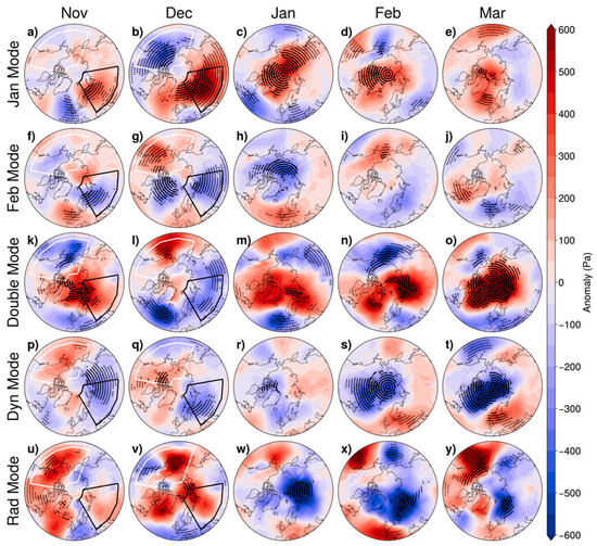
Figure 3.
Monthly mean of MSLP anomaly from 40° N poleward in the northern hemisphere for the different modes from November to March: (a–e) January mode, (f–j) February mode, (k–o) Double mode, (p–t) Dynamical mode, and (u–y) Radiative mode. Blue and red shaded regions correspond to negative and positive MSLP anomalies, respectively. Stippled areas show statistical confidence at the 95% level according to a Wilcoxon signed-rank test. Black and white boxes indicate the Ural and the extended Aleutian regions, respectively.

Table 1.
Mean MSLP anomaly for the Ural and Aleutian regions for the different modes in November and December.
For the January mode, it can be observed that winters begin in November, with a few regions of high significance (see Figure 3a): a positive anomaly over the Barents Sea and a negative anomaly in Western Europe. In December (see Figure 3b), significant signals are found across the investigated area. Therefore, winters typically exhibit a pressure dipole with strong positive anomalies over Siberia, Asia, and the North Atlantic, while significant negative anomalies cover the center and Northwest America. Thus, a positive anomaly of +395 Pa is found in the Ural region, while a negative anomaly of around −190 Pa is found in the Aleutian region in December (see Table 1). These early signals bear resemblance to the Ural blocking events identified in previous studies, associating them with wavenumber 1 propagation and negative AO tropospheric response [21,24]. Interestingly, these surface signals display a wave-1-like pattern, coinciding with significant wave-1 activity diagnosed by M22 in the midst of the stratosphere before the occurrence of important SSWs for the January mode (see their Figure 8a). Thus, these results suggest that the surface patterns observed in November and December act as precursors to an important SSW in January, which, in turn, impacts the surface in the following months. Indeed, in January (see Figure 3c), strong positive anomalies are observed at the pole and Eastern Siberia, while negative anomalies are found in Southern Europe and Northeast America. This pattern is typical of the negative phase of the AO generated after SSWs. It is consistent with the NAM indices, showing a downward propagation of positive anomalies in January (see Figure 1a). This negative AO-like pattern is maintained until March, indicating the sustained influence of this important SSW on the tropospheric weather (Figure 3d,e).
Regarding the February mode, surprisingly, opposite signals compared to the January mode are found, particularly from November to January (Figure 3f–h), confirming that these two modes possess very different initial surface conditions. In November, winters tend to have a negative anomaly over the Barents Sea, while a positive anomaly is observed in Western Europe. In December, the previous negative anomaly covers a portion of Siberia, and another negative anomaly appears over the west of Greenland, while a positive anomaly is observed over the U.S. West Coast and Pacific Ocean. Thus, we found a negative anomaly of −180 Pa in the Ural region, while a positive anomaly of +118 Pa characterized the Aleutian region in December (see Table 1). Interestingly, this surface anomaly exhibits a wave-2-like pattern, especially for the negative signals, aligning with the period when wave-2 activity in the stratosphere increases for this mode (Figure 8b in M22). Therefore, oppositely to the January mode, this surface pattern in December serves as an indicator of a future strong vortex generated in January. More generally, these results support the idea that November and December are crucial months for identifying and anticipating the occurring mode. In January, a negative anomaly is present at the pole, while a positive anomaly is observed in Western Europe and the North Atlantic. This pattern resembles to the positive phase of the AO. Consistent with the NAM evolution obtained for the February mode (Figure 1b), no significant negative phase of AO is found in February when the important SSW is expected to occur (Figure 3i), confirming that the anomaly does not reach the surface. Only positive anomalies are found in the North Pacific region. Interestingly, the Pacific blocking region emerges both in the pre- and post-warming phases, as highlighted by Bancalá et al. [21] for wave-2 SSW events. Unexpectedly, in March (Figure 3j), significant signals appear again with a wave-2-like pattern, as seen in early winter. These may be caused by regular weather anomalies that are contributions of quasi-stationary wave-1 and wave-2 events propagating in winter [17] and planetary wave reflection in the stratosphere [26]. Additionally, these results align with the conclusions mentionned earlier and reported in Monnin et al. [39] regarding the impact of the timing of SSWs on the subsequent tropospheric events.
Unlike the January and February modes, the Double mode exhibits strong signals in November (Figure 3k), with a positive anomaly over the pole and the Barents Sea, while negative anomalies cover Southern Europe and the Bering Sea. Indeed, a strong positive anomaly of +310 Pa is found in the Ural region, while a negative anomaly of −88 Pa is present in the Aleutian region in November (see Table 1). This pattern shares similarities with the one observed in December for the January mode; i.e., a wave-1-like pattern with a blocking event in the Bering sea that can act as a precursor to the expected important SSW in the following month. In December (Figure 3l), significant negative anomalies with a wave-1-like pattern cover the North Atlantic Ocean and Eurasia, while a positive anomaly is present over the Bering Sea. Although the first important SSW occurs in December, there is no immediate downward propagation of the positive anomaly, as shown in Figure 1c, where the descent into the troposphere occurs later in January and February (Figure 3m,n).
Finally, in March (Figure 3o), a negative phase of the AO is observed, again due to the effects of the second important SSW, with a significant positive anomaly covering the entire pole, Greenland, and a northern part of Siberia.
Although the pressure patterns found in November are not responsible for FSW events occurring in March and April in the unperturbed scenarios, it is nevertheless interesting to investigate how unperturbed winters tend to behave at the surface in early winter.
Concerning the Dynamical mode, during November (Figure 3p), surface anomaly signals display statistically significant anomalies, albeit of modest magnitudes. These anomalies consist of negative signals over Siberia and the Atlantic Ocean, contrasted by a positive signal in the Pacific Ocean. Thus, −166 Pa is found over the Ural region, and approximately +100 Pa is found in the Aleutian region in November. By December (Figure 3q), a positive Pacific North America pattern appears, with significant negative signals of around −180 Pa over the Ural region (see Table 1). It is worth noting that these patterns resemble those found in the same period in the February mode, which may indicate an upcoming strong vortex event [24]. On the other hand, in January (Figure 3r), no significant MSLP anomalies are present, suggesting that there is no typical evolution among winters during this month. However, in February and March (Figure 3s,t), significant MSLP anomalies reappear. These two months exhibit similar patterns, characteristic of a positive AO. The positive AO phase in the Dynamical mode likely results from the downward propagation of stratospheric anomalies, confirming their connection with strong vortex events. Moreover, the surface signal in the Dynamical mode reveals a wave-1-like pattern, consistent with the wave activity diagnosed in the stratosphere during this period (Figure 8a in M22).
While the Radiative mode consists of only five winters, it offers an interesting perspective on MSLP anomalies, particularly when substantial signals spread over extensive regions. Notably, the Radiative mode presents significant positive anomaly signals over North America, the Pacific Ocean, and Greenland in November (Figure 3u). Of particular interest are the positive signals found in the Pacific region, which are also present in the Dynamical and February modes in December. Notably, the Aleutian region is characterized by positive anomalies of +160 and +130 Pa in November and December, respectively. Most importantly, these signals are opposite to those found within the January and Double modes in December and November, respectively, confirming that the MSLP anomalies in North Pacific region in early winter are crucial for the upcoming stratrosphere evolution, as already underscored in previous studies (e.g., [53]). In December and January (Figure 3v,w), the Radiative mode exhibits only small regions with statistically significant signals, making it challenging to establish a clear trend among the associated winters. In February and March (Figure 3x,y), the signals begin to deviate noticeably from the positive AO pattern observed in the Dynamical mode. Unlike the Dynamical mode, the NAM evolution of the Radiative mode indicates that the surface patterns in February and March are less influenced by the stratosphere due to the less-significant descent of anomalies during these months. Nevertheless, the final observed positive anomaly descent in the NAM evolution in April (Figure 2b) indicates that the surface is affected a month later in a manner consistent with that observed in the Dynamical mode.
Thus, based on Figure 3, it is evident that these five modes exhibit known blocking patterns within their distinct regular surface pressure anomalies, which are consistent with strong vortex and weak vortex events. Notably, among the perturbed modes, there are similarities in the initial surface conditions and surface impacts between the January and Double modes, which are opposite to those observed for the February mode. Specifically, for the Double and January modes, a wave-1-like pattern is present at the surface in November and December, respectively, and the positive pressure anomaly tends to propagate from the stratosphere to the surface after an important SSW, generally inducing a negative phase of the AO. In contrast, the February mode displays a wave-2-like pattern at the surface in December and a positive phase of AO in January. The quasi-absence of significant signals in February indicates that there are no typical similar patterns among winters associated with this mode during this month. Therefore, it appears that certain early-winter (November/December) MSLP anomalies are involved in significant downward impacts in scenarios where important SSWs occur early (December/January). More broadly, the early winter surface conditions within the February and Dynamical modes share similar signals—in particular over the Ural region—that are opposite to the January and Double modes. These findings are in agreement with previous studies underlying, in particular, the Ural mountains and North Pacific as crucial blocking regions, announcing the upcoming weak vortex and strong vortex events in the next weeks [24,25,53].
3.2.2. Lead–Lag Correlations between Stratospheric Modes and Regional Blocking
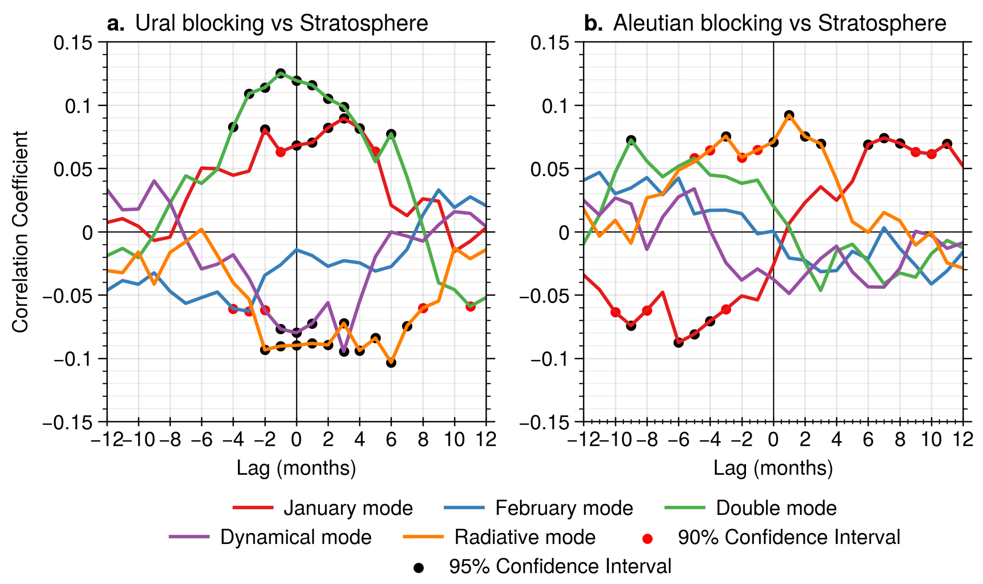
The connections between the different modes and both the Ural and Aleutian regions are further explored through lead–lag correlation coefficients, as illustrated in Figure 4. This analysis focuses on significant coefficients within at least the 90% confidence interval. Overall, the Ural region proves more influential and sensitive than the Aleutian region in stratosphere–troposphere coupling among the modes, aligning with previous studies (e.g., [13,29,46]). Consistent with MSLP anomaly maps (Figure 3), these results demonstrate that Ural blocking uniquely correlates with the subsequent occurrence of the January and Double modes in the stratosphere. Conversely, negative MSLP anomalies in the Ural region indicate the onset of February or unperturbed modes. When the stratosphere begins to lead, Ural blocking persists for up to six months in the January and Double modes, while it is absent in other modes. Notably, in unperturbed modes, the negative MSLP anomaly endures for up to three months (see Figure 4a). This suggests that Ural blocking or Ural trough conditions are self-perpetuating, maintained by the descent of stratospheric anomalies caused by SSW or strong polar vortex events, respectively. A similar pattern is observed for Aleutian blocking, but only in the Radiative mode (see Figure 4b). Intriguingly, a strong Aleutian trough from −10 to −3 months precedes the January mode in the stratosphere, which subsequently generates Aleutian blocking from +6 to +11 months. This result is consistent with the conclusions in Bancalá et al. [21], who reported the emergence of the Pacific blocking in the post-warming phase. Thus, both the Ural and Aleutian regions appear to influence the January mode and stratosphere–troposphere coupling throughout winter and beyond.

Figure 4.
The lead–lag correlation coefficients between the (a) Ural blocking index and modes and between the (b) Aleutian blocking index and modes. The correlation coefficients within the 90% and 95% confidence intervals, as determined by a t-test, are indicated in red and black, respectively.
The February mode exhibits markedly different behavior compared to the January and Double modes, as it is not triggered by Ural or Aleutian blocking. Instead, it displays a Ural trough from −4 to −3 months, similar to the pattern observed in the unperturbed modes from −2 months onward (see Figure 4a). This suggests that the February mode initially resembles an unperturbed mode before experiencing a later SSW. The February mode’s development appears largely independent of the Aleutian region (see Figure 4b). Finally, the SSW associated with the February mode does not significantly impact the Ural and Aleutian regions, further underscoring the potentially weak surface effects of this warming event.
Since both perturbed and unperturbed modes demonstrate MSLP anomalies exhibiting wave-like patterns with typical blocking events that are known to impact the planetary wave activity, in the next section, we examine the propagation of planetary wavenumbers 1 and 2 through the EP flux to better understand the dynamical forcing within each mode.
3.3. Eliassen–Palm Flux Analysis of Planetary Wave Dynamics
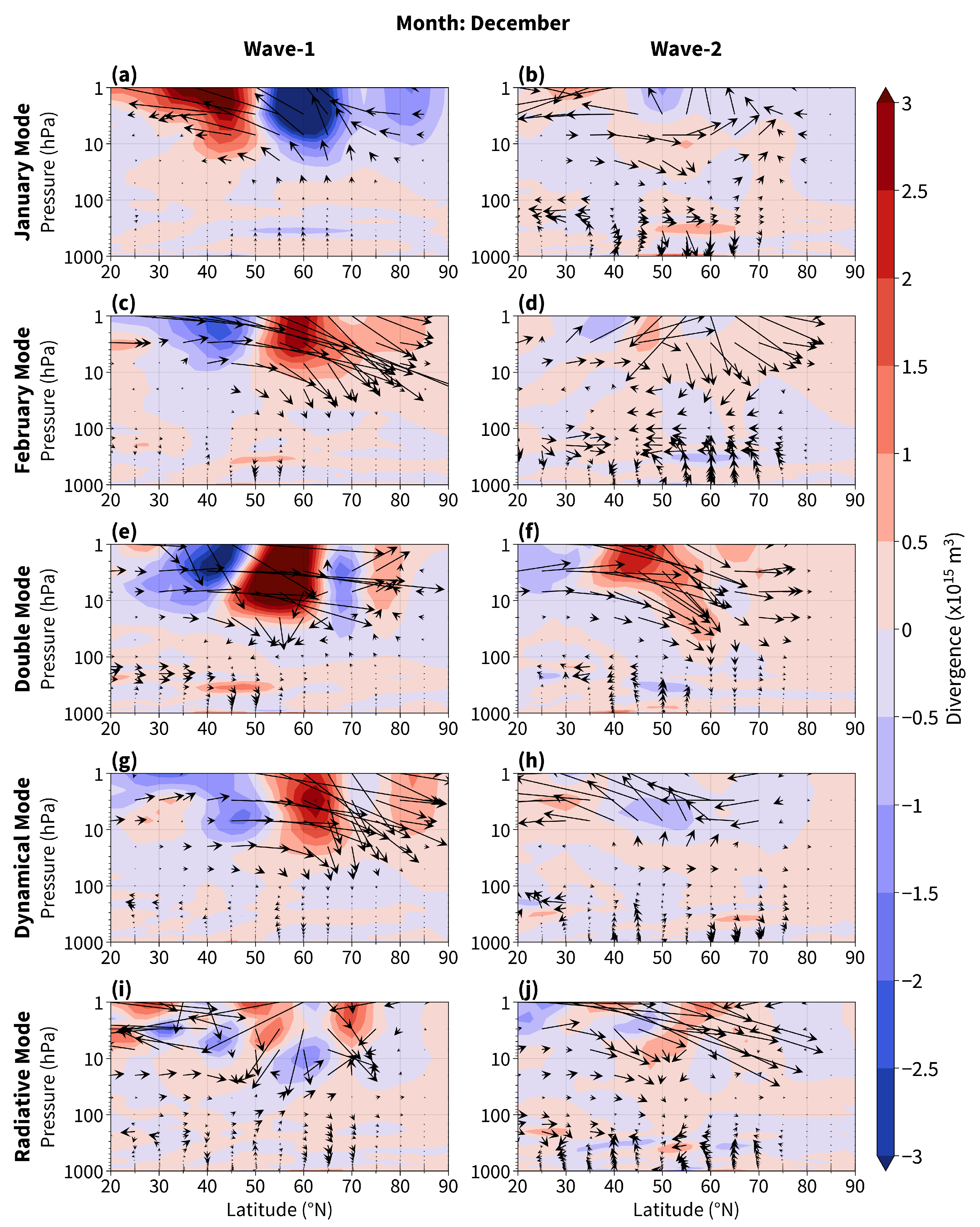
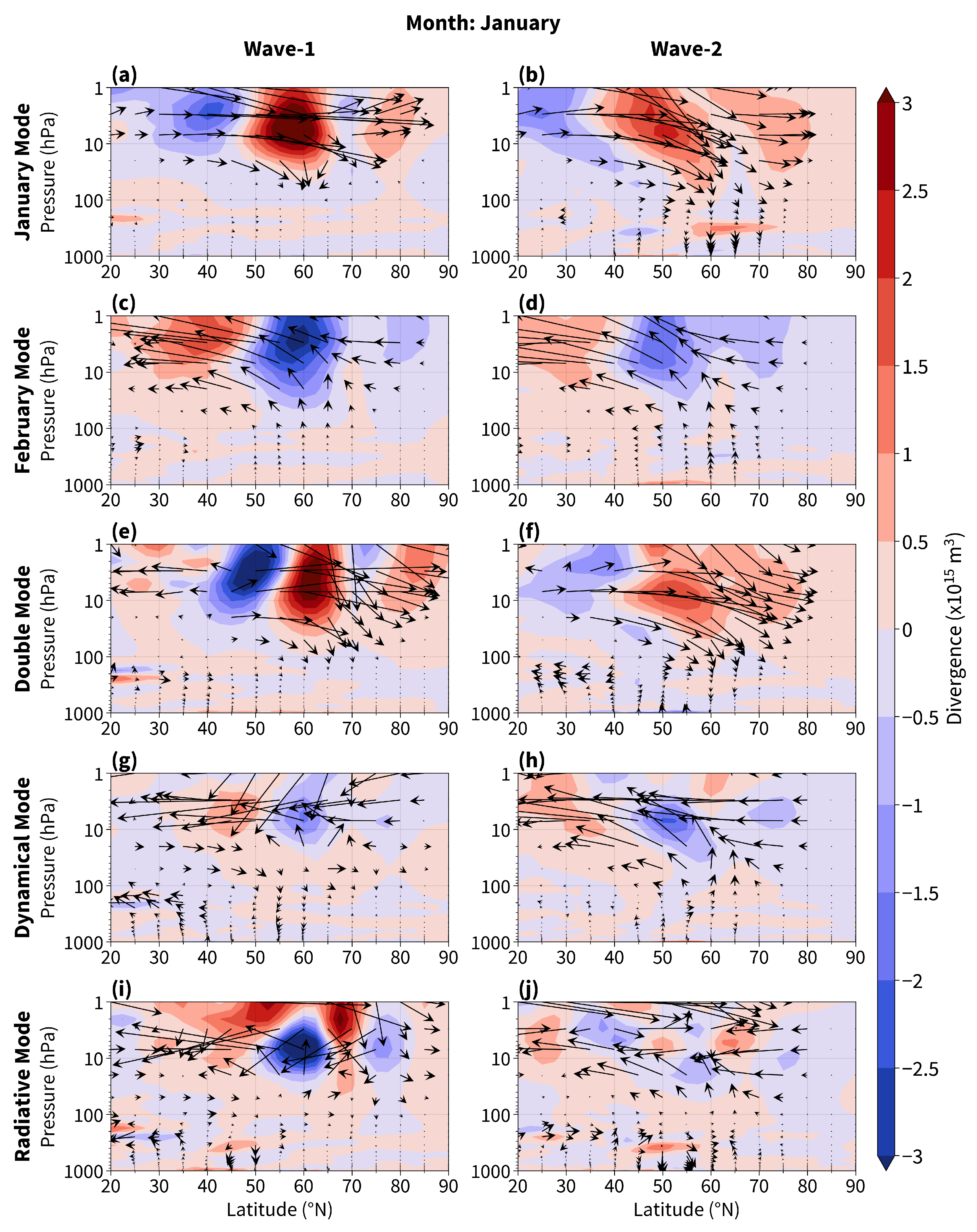
Figure 5 and Figure 6 show the decomposition of wavenumbers 1 and 2 of the EP flux and of its divergence in December and January, respectively, for the five modes. Figure 7 shows the same results but for the other months for certain modes that are interesting to analyze. The EP flux vectors indicate the propagation direction of planetary waves in the vertical–meridional plan. The convergence (blue) and divergence (red) of the EP flux depicts areas with deceleration and acceleration of the zonal wind, respectively. Here, we will present the results mainly located between 40 and 70° N, corresponding to the edge of the polar vortex, where the interaction between planetary waves and mean flow is important.
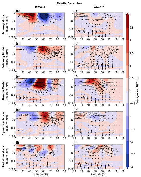
Figure 5.
Decomposition of wavenumbers 1 and 2 of the mean latitude–height anomaly of the EP flux and of the mass–weighted divergence of EP flux for the different modes in December: (a,b) January mode, (c,d) February mode, (e,f) Double mode, (g,h) Dynamical mode, and (i,j) Radiative mode. EP flux vectors (arrows) indicate the magnitude of the planetary waves activity and their propagation. Shaded negative (blue) and positive (red) values correspond to a deceleration and acceleration of the zonal wind, respectively.
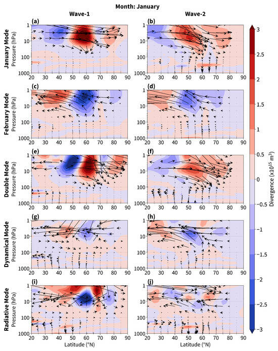
Figure 6.
Decomposition of wavenumbers 1 and 2 of the mean latitude–height anomaly of the EP flux and of the mass–weighted divergence of the EP flux for the different modes in January: (a,b) January mode, (c,d) February mode, (e,f) Double mode, (g,h) Dynamical mode, and (i,j) Radiative mode. EP flux vectors (arrows) indicate the magnitude of the planetary waves activity and their propagation. Shaded negative (blue) and positive (red) values correspond to deceleration and acceleration of the zonal wind, respectively.
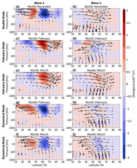
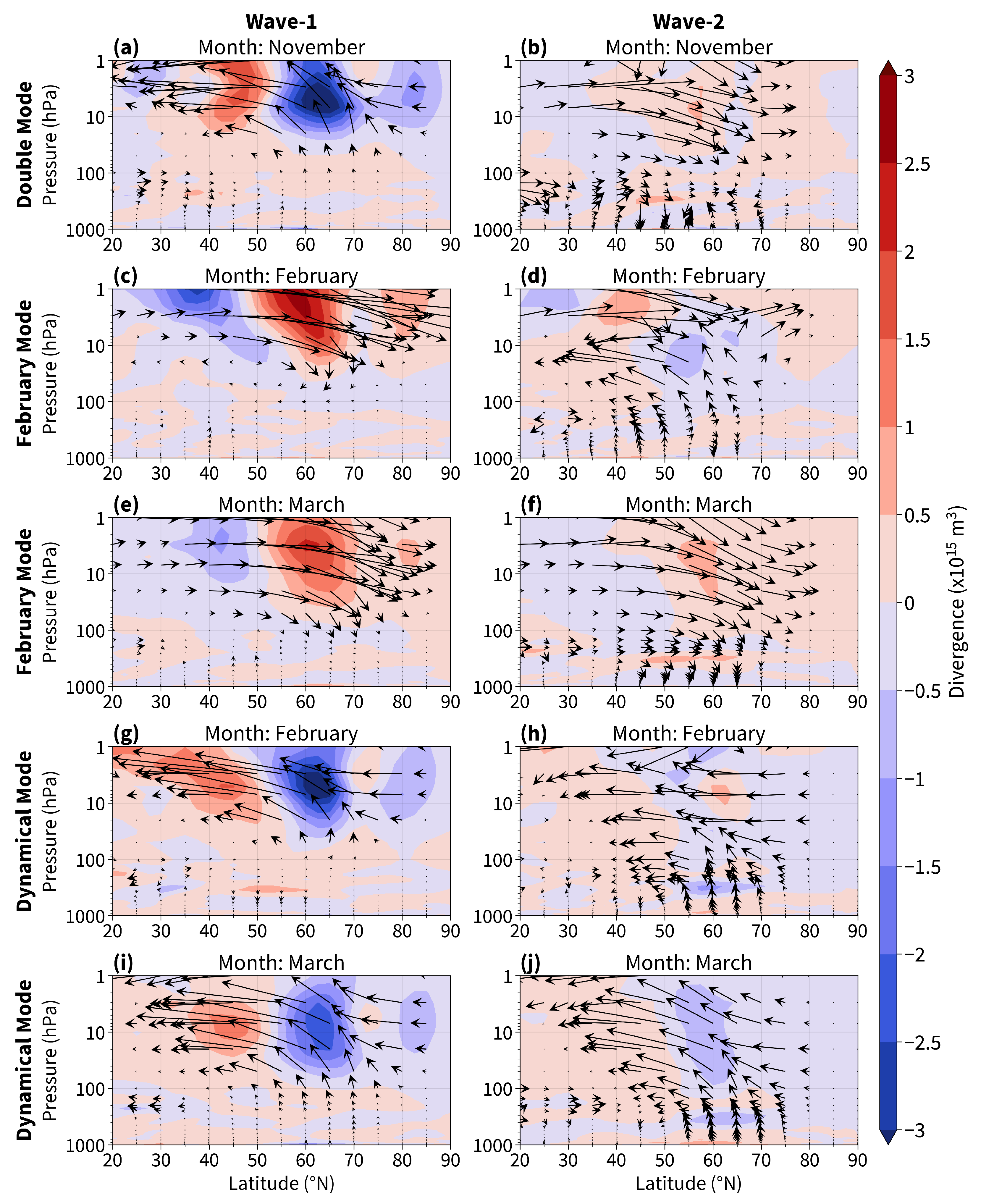
Figure 7.
Decomposition of wavenumbers 1 and 2 of the mean latitude–height anomaly of the EP flux and of the mass–weighted divergence of the EP flux for the Double mode in November (a,b), the February mode in February (c,d) and March (e,f), and the Dynamical mode in February (g,h) and March (i,j). EP flux vectors (arrows) indicate the magnitude of the planetary waves activity and their propagation. Shaded negative (blue) and positive (red) values correspond to deceleration and acceleration of the zonal wind, respectively.
Overall, the EP flux vectors in the stratosphere, particularly those found in wave-1 flux, are typical during SSW events; i.e., upward and equatorward wave propagation is observed during the prewarming phase, while downward and poleward propagation is observed during the SSW and recovery phases (e.g., [48]).
Concretely, the dynamical activities diagnosed both in the pre and post-warming phases yield an initial explanation of the role of wave-1 and wave-2 in the occurrence or lack of important SSWs and in the subsequent surface impacts for each mode. Indeed, in December, the January mode is characterized by a strong upward and equatorward wave-1 flux from the troposphere, causing a strong wind deceleration in the stratosphere, whereas wave-2, propagating mostly poleward, does not seem to play a role (Figure 5a,b). As a result, it seems that the important SSW occurring in January is mostly triggered by the propagation of wave-1, as mentioned in M22. Interestingly, this dynamical condition is similar to the one observed in November in the Double mode, suggesting that the first important SSW in December is also caused by wave-1 (see Figure 7a,b). Thus, the downward and poleward propagation of wave-1 and wave-2 found in December for the Double mode (Figure 5e,f) is consistent with the theory stating that planetary waves cannot propagate upward in easterlies conditions [4], as well as with the planetary wave reflection caused by important SSWs [26]. Moreover, these strong downward propagations potentially represent the reflection of waves that may subsequently impact the surface weather [21]. Similar downward wave propagations are found in January for the January mode, when the important SSW is supposedly occurring (Figure 6a,b). Since the negative phase of the AO-like pattern tends to manifest at the surface after the important SSWs in the Double and January modes (see Figure 3c,d,m), these results argue in favor of wave-1 and wave-2 reflections as necessary physical processes for the emergence of these surface signals. This hypothesis is strengthened by the EP flux diagnosed in February for the February Mode (see Figure 7c,d), when the important SSW is occurring, exhibiting a downward and poleward wave-1 propagation. However, a simultaneous upward and equatorward wave-2 propagation is therefore likely responsible for the absence of significant surface impacts during this period. Surprisingly, this opposition between wave-1 and wave-2 disappears in March (see Figure 7e,f), when both display a downward and poleward flux, suggesting that the significant surface signals found during this period (see Figure 3j) are partly due to these downward wave fluxes.
Overall, the February mode appears to be very different from the January and Double modes regarding dynamical aspects. Indeed, surprisingly, in December, we can observe that the February and Dynamical modes possess similar downward and poleward wave-1 fluxes from the stratosphere to the surface; however, with opposite wave-2 propagations (see Figure 5c,d,g,h). Since this dynamical behavior is found during a period when both of these modes experience reinforcement of the polar vortex, these results suggest that the downward–poleward wave-1 propagation is leading the dynamics in the stratosphere. This inference is endorsed in the next month in January, where the February and Dynamical modes show similar upward and equatorward wave-2 fluxes, but, this time, with opposite wave-1 propagations, particularly in the troposphere (see Figure 6c,d,g,h). Indeed, the February mode exhibits a strong upward–equatorward wave-1 flux, in addition to the wave-2 flux, which is very likely responsible for the occurrence of important SSWs in February. Hence, unlike the January and Double modes, the important SSW of the February mode is triggered by a combined effect from upward wave-1 and wave-2 fluxes, inducing a strong wind deceleration.
Thus, apparently, the weak wave-1 activity in the Dynamical mode in January indicates that the vortex will remain strong the next month (Figure 6g,h). Interestingly, the Dynamical mode exhibits a reinforcement from February to March in its upward and equatorward wave-1 and wave-2 fluxes, explaining the occurrence of the dynamical FSW with an early timing (Figure 7g–j). Thus, the Dynamical mode presents similarities, with the important SSW occurring in the February mode with regard to the contributions of wave-1 and wave-2 activities, but with less intensity. Therefore, this EP flux analysis illustrates the similar dynamical aspect of this FSW to classical mid-winter important SSW. In April, no strong downward EP fluxes are found, confirming that this last dynamical FSW does not impact the surface. In contrast, the Radiative mode does not demonstrate any strong upward wave-1 or wave-2 fluxes throughout winter, as expected. However, these observed features may simply arise from the small sample size and the lack of alignment in the timing of minor deceleration/acceleration events among the five winters.
In light of these results, it appears that an enhancement of wave-1 activity in November and December is pivotal for the subsequent stratospheric evolution and the tropospheric evolution. Thus, these diagnosed EP fluxes provide a physical explanation to connect the observed early winter surface signals with the timing of important SSWs and their potential surface impacts. In the next section, we discuss these results by comparing them with the existing literature and provide our conclusions.
4. Discussion
Overall, the results reported here demonstrate particular stratosphere–troposphere coupling within the main stratospheric modes established in M22. Notably, these modes exhibit distinct surface precursors in early winter, connected with particular dynamical activities that determine the timing of important SSWs. Additionally, our results underscore the importance of the timing of important SSWs in the following tropospheric responses. For instance, as depicted in Figure 1, it is clear that important SSWs occurring in January are propagating up to the surface, whereas important SSWs occurring later in February do not display evident stratospheric anomaly descents. Furthermore, according to Figure 3, it seems that this descent of important SSWs occurring in January is generally followed by more pronounced surface impacts than important SSWs occurring later in February [6]. Therefore, this result potentially supports the role of the timing of important SSWs in the following tropospheric impacts, as underscored in Monnin et al. [39]. According to the authors, early winter SSWs (December/January) experience stronger polar vortex anomalies more often, since the stratospheric mean state is stronger than for late winter SSWs (February/March). However, although Monnin et al. [39] found that early SSWs (December/January) do not propagate further downward than late SSWs (February/March), contrasting with our results, it is probable that this finding is the result of disparate downward propagations among winters composing the February mode. Thus, an investigation of the correlation between downward propagation and surface impacts is needed to confirm this hypothesis.
Importantly, our findings show that the different modes possess specific surface weather conditions in early winter. Indeed, the MSLP anomalies found in November and December confirm the role of certain blocking regions on the subsequent stratospheric evolutions already underscored in previous studies. Notably, the persistent Ural blocking anomalies in November and December within the Double and January modes, respectively, are consistent with Peings [24], who found that this pattern is associated with increased upward planetary waves into the stratosphere, leading to SSWs. Similarly, our findings align with the conclusions of Kohler et al. [25], who found that the MSLP in the Ural and Aleutian regions are negatively and positively correlated with the strength of the polar vortex up to two months, respectively. Moreover, as underlined in Peings [24], the stratospheric response to the Ural blocking in November tends to penetrate into the troposphere, increasing the occurrence of the negative North Atlanctic Oscillation in December and January. These latter tendencies are well-retrieved here through the January and Double modes, strengthening the prediction skill of these regions. It is noteworthy that the Double mode presents unique, strong stratosphere–troposphere coupling from November, with important surface impacts following important SSW events up to March. This highlights the singularity of this mode.
The analysis of the lead–lag correlation coefficients between the Ural and Aleutian regions and each mode confirmed these tendencies and provided a more comprehensive picture of their connections. Indeed, the sign of the MSLP anomaly in the Ural region appears to be a determining factor for the upcoming stratospheric mode up to four months in advance. This examination offers valuable information for anticipating the different modes. Interestingly, although an Ural trough generally precedes the February mode by 3 to 4 months, this mode is not triggered by Ural or Aleutian blocking. This suggests that other underlying mechanisms are at play for this mode. Moreover, the February mode shows no impact on the Ural or Aleutian regions from the stratosphere, underscoring the absence of descending stratospheric anomalies after the important SSW characterizing this mode. Therefore, the occurrence of the February mode remains enigmatic. Future research should investigate why an apparently unperturbed mode suddenly transitions into a perturbed state. This peculiar behavior warrants further exploration to elucidate the mechanisms driving the February mode’s development and evolution.
Furthermore, the MSLP anomalies with wave-like patterns diagnosed in November and December also seem consistent with the wave activity preconditioning weak vortex and strong vortex events reported in previous studies [21,23,40]. For instance, the MSLP anomalies and wave activities examined here agree with the results in Bancalá et al. [21], stating that blocking events in the Euro-Atlantic sector lead to wave-1 warmings, while those in the Pacific region precede and follow wave-2 warmings, combining wave-1 and wave-2 activities. Additionally, the planetary wave activity analysis carried out here aligns overall with the conclusions reported in Díaz-Durán et al. [40]. Indeed, they found an enhancement and inhibition of wave-1 activity for weak vortex and strong vortex events in early winter (October/Novmber/December), respectively, which is observed among the different modes during this period. However, since Díaz-Durán et al. [40] mixed weak vortex events occurring in mid (January/February) and late winter, they found that these events present an enhancement of wave-1 and wave-2 events, while this dynamical behavior corresponds to those occurring in the February and Dynamical modes but not in the January mode. Therefore, it is noteworthy that weak vortex events occurring in January and February must be classified separately when studying seasonal variability throughout winter.
The subsequent analysis of EP flux yields a better understanding of the stratospheric responses to particular vertical wave propagation occurring within each mode in the pre-warming and recovery phases. Here, the planetary wave activities analyzed demonstrate that the January and Double modes bear similarities with the absorbing SSW type, while the February mode more closely resembles a reflecting SSW type, as described in Kodera et al. [26]. It is noteworthy that both the January and Double modes exhibit downward and poleward wave-1 and wave-2 propagations during the important SSW, even though they are only generated by upward and equatorward wave-1 propagation. Conversely, the February mode displays only a wave-1 reflection in February when the important SSW is happening, while wave-2 is still propagating upward and equatorward. These results indicate potential nonlinear wave–wave interaction in the stratosphere, modifying the zonal wave number during the SSW event [26,53]. Moreover, the conclusions reported in Huang et al. [53] suggest that the shorter time-scale strong vortex events found in the February mode are caused by linear wave interference, whereas longer time-scale strong vortex events in the Dynamical and Radiative modes result from nonlinear wave interference. However, further investigations are required to confirm this hypothesis.
Finally, the polar vortex geometry within the different modes does not appear to determine the understanding stratosphere–troposphere coupling, even though no precise examination was performed here. Indeed, the January and February modes bear resemblance to the findings of Splitting and Displaced events in Mitchell et al. [15] (see their Figure 4), respectively, and they are also consistent with their seasonal distribution of splitting, displacement, and mixed events (see their Figure 3). However, the planetary wave activity related to these two scenarios, mainly wave-1 driven for the January mode and both wave-1 and wave-2 driven for the February mode, are in contradiction with this agreement. It is therefore difficult to attribute a specific polar vortex geometry to winters associated with these scenarios without making assumptions with significant uncertainties. Furthermore, since the difference found in impacting the troposphere between split and displaced events is very sensitive to the SSW definition [12,17,18], the polar vortex geometry appears to be less decisive than the persistence of the anomaly in the tropopause region [28], the absorption of planetary waves [26], or potentially, the timing of important SSWs in predicting stratospheric anomaly descents and surface impacts.
5. Conclusions
This study examined stratosphere–troposphere coupling through an analysis of the January, February, Double, Dynamical, and Radiative polar vortex modes identified in M22. The principal findings can be summarized as follows:
- As precursors, the January and Double modes present Ural blocking and Aleutian trough events in December and November, respectively, associated with an upward–equatorward wave-1 propagation, while the February and Dynamical modes display Ural trough and Aleutian blocking events during this period, associated with a downward–poleward wave-1 propagation. Specifically, the Radiative mode exhibits a significant Aleutian blocking event as a precursor in November and December.
- In the pre-warming phases, the January and Double modes display upward–equatorward wave-1 and downward–poleward wave-2 propagations, while the February and Dynamical modes show upward–equatorward wave-1 and wave-2 propagations.
- During warming, the January and Double modes exhibit downward and poleward wave-1 and wave-2 propagations, associated with negative AO-like responses, while the February mode displays downward–poleward wave-1 and an upward–equatorward wave-2 propagations without generating particular tropospheric responses.
- In the recovery phase, the February mode displays a downward–poleward propagation of both wave-1 and wave-2, which is associated with a slight surface impact outside the Ural and Aleutian regions.
This analysis reveals that the Ural region plays a pivotal role in the occurrence of the different modes, while the Aleutian region appears to be less determinant in this process. The January and Double modes exhibit positive correlations with Ural blocking, characterized by substantial positive MSLP anomalies: approximately +400 Pa in December for the January mode and +300 Pa in November for the Double mode. Conversely, the February and Dynamical modes display negative MSLP anomalies in the Ural region during November and December, ranging from −80 to −180 Pa for the February mode and from −166 to −184 Pa for the Dynamical mode. Notably, the Radiative mode appears to be the only mode triggered by the Aleutian blocking, with significant positive MSLP anomalies in the Aleutian region ranging from +160 to 135 Pa from November to December. Intriguingly, the February mode is not triggered by Ural or Aleutian blocking, suggesting that other mechanisms are at play. This raises questions about why an apparently unperturbed mode generates an important SSW; a phenomenon that warrants further investigation.
Our analysis suggests that strong upward and equatorward wave-1 activity in early winter (November/December) is likely to result in a winter characterized by the Double or January modes. Conversely, if there is no strong wave-1 forcing, we can expect a winter dominated by the February or Dynamical modes, which are generally both wave-1 and wave-2-driven. It thus appears that important SSWs occurring in the January and Double modes differ significantly from those occurring in the February mode, whether in terms of the dynamical activity observed in the pre-warming phase or the tropospheric responses generated. Indeed, important SSW events occurring in the January and Double modes, which are associated with downward–poleward wave-1 and wave-2 propagations, tend to impact the surface more significantly, generating negative AO phases, than those occurring in the February mode, associated with downward–poleward wave-1 and upward–equatorward wave-2 propagations during warming. This underscores the important role of timing in this process. However, even though early winter important SSWs (December/January) have a greater overall impact on the surface than late winter important SSWs (February/March), it is noticeable that those occurring in the Double mode impact the surface until March. This inconsistency may be the result of the particularly strong stratosphere–troposphere coupling happening in the Double mode, emphasizing its singularity. In conclusion, our findings provide a novel perspective on the stratosphere–troposphere coupling through these various modes, which are initialized by specific surface patterns in November and December, announcing the timing of important SSWs. Moreover, this latter factor appears to be a key determinant of the subsequent tropospheric responses. Hence, these outcomes may have potential applications for sub-seasonal to seasonal climate forecasts.
Future research should employ mechanistic models to test the hypothesis that these precursors and specific wave activities associated with each mode can simulate important SSWs with the expected timing. Moreover, an investigation into the causes of stratospheric anomaly entry into the troposphere would be advantageous. Further investigation is required to gain a deeper understanding of the triggers for each mode. One potential avenue for exploration is the examination of links between sea ice concentrations and thicknesses and snow cover at the beginning of winter, as proposed by [24]. Finally, future research should investigate the nonlinear interactions between each mode and other known influences on planetary wave activity throughout the winter, such as the El Niño–Southern Oscillation (ENSO) and the Quasi-Biennial Oscillation (QBO).
Author Contributions
Conceptualization, P.K., A.H. and A.M.; methodology, P.K., A.H. and A.M.; validation, P.K., A.H. and A.M.; formal analysis, A.M.; investigation, A.M.; writing—original draft preparation, A.M.; writing—review and editing, A.M.; visualization, A.M.; supervision, P.K. and A.H.; project administration, P.K. and A.H. All authors have read and agreed to the published version of the manuscript.
Funding
This research received no external funding.
Institutional Review Board Statement
Not applicable.
Informed Consent Statement
Not applicable.
Data Availability Statement
The ERA5 data on single levels and pressure levels were accessed on 1 February 2023 from the Copernicus Climate Data Store [54] and are available at https://doi.org/10.24381/cds.adbb2d47 and https://doi.org/10.24381/cds.bd0915c6 (accessed on 1 July 2024), respectively.
Acknowledgments
This work was performed within the framework of the European ARISE project and was funded by the French Educational Ministry with EUR IPSL.
Conflicts of Interest
The authors declare no conflicts of interest.
Appendix A
- January single-warming mode: 1950/1951, 1952/1953, 1954/1955, 1959/1960, 1967/1968, 1969/1970, 1970/1971, 1976/1977, 1984/1985, 1997/1998, 2001/2002, 2002/2003, 2003/2004, 2005/2006, 2011/2012, 2012/2013, 2018/2019
- February single-warming mode: 1956/1957, 1957/1958, 1962/1963, 1972/1973, 1978/ 1979, 1980/1981, 1982/1983, 1986/1987, 1988/1989, 1989/1990, 1990/1991, 1994/1995, 2007/2008, 2008/2009, 2009/2010, 2016/2017, 2017/2018
- Double warmings mode: 1951/1952, 1965/1966, 1968/1969, 1979/1980, 1987/1988, 1998/1999, 2000/2001
- Dynamical final warming mode: 1955/1956, 1958/1959, 1960/1961, 1963/1964, 1973/ 1974, 1974/1975, 1975/1976, 1985/1986, 1992/1993, 1995/1996, 1999/2000, 2010/2011, 2013/2014, 2014/2015, 2015/2016
- Radiative final warming mode: 1961/1962, 1964/1965, 1966/1967, 1996/1997, 2019/ 2020
- Unclassified winters: 1953/1954, 1971/1972, 1977/1978, 1981/1982, 1983/1984, 1991/ 1992, 1993/1994, 2004/2005, 2006/2007
References
- Sigmond, M.; Scinocca, J.; Kharin, V.; Shepherd, T. Enhanced seasonal forecast skill following stratospheric sudden warmings. Nat. Geosci. 2013, 6, 98–102. [Google Scholar] [CrossRef]
- Domeisen, D.I.; Butler, A.H.; Charlton-Perez, A.J.; Ayarzagüena, B.; Baldwin, M.P.; Dunn-Sigouin, E.; Furtado, J.C.; Garfinkel, C.I.; Hitchcock, P.; Karpechko, A.Y.; et al. The Role of the Stratosphere in Subseasonal to Seasonal Prediction: 1. Predictability of the Stratosphere. J. Geophys. Res. Atmos. 2020, 125, e2019JD030920. [Google Scholar] [CrossRef]
- Waugh, D.W.; Sobel, A.H.; Polvani, L.M. What Is the Polar Vortex and How Does It Influence Weather? Bull. Am. Meteorol. Soc. 2017, 98, 37–44. [Google Scholar] [CrossRef]
- Matsuno, T. A Dynamical Model of the Stratospheric Sudden Warming. J. Atmos. Sci. 1971, 28, 1479–1494. [Google Scholar] [CrossRef]
- Butler, A.H.; Sjoberg, J.P.; Seidel, D.J.; Rosenlof, K.H. A sudden stratospheric warming compendium. Earth Syst. Sci. Data 2017, 9, 63–76. [Google Scholar] [CrossRef]
- Baldwin, M.P.; Dunkerton, T.J. Stratospheric Harbingers of Anomalous Weather Regimes. Science 2001, 294, 581–584. [Google Scholar] [CrossRef]
- Baldwin, M.P.; Thompson, D.W. A critical comparison of stratosphere–troposphere coupling indices. Q. J. R. Meteorol. Soc. 2009, 135, 1661–1672. [Google Scholar] [CrossRef]
- Thompson, D.W.J.; Wallace, J.M. Regional Climate Impacts of the Northern Hemisphere Annular Mode. Science 2001, 293, 85–89. [Google Scholar] [CrossRef]
- Butler, A.H.; Domeisen, D.I.V. The wave geometry of final stratospheric warming events. Weather Clim. Dyn. 2021, 2, 453–474. [Google Scholar] [CrossRef]
- Butler, A.H.; Seidel, D.J.; Hardiman, S.C.; Butchart, N.; Birner, T.; Match, A. Defining Sudden Stratospheric Warmings. Bull. Am. Meteorol. Soc. 2015, 96, 1913–1928. [Google Scholar] [CrossRef]
- Butler, A.H.; Gerber, E.P. Optimizing the Definition of a Sudden Stratospheric Warming. J. Clim. 2018, 31, 2337–2344. [Google Scholar] [CrossRef]
- Charlton, A.J.; Polvani, L.M. A New Look at Stratospheric Sudden Warmings. Part I: Climatology and Modeling Benchmarks. J. Clim. 2007, 20, 449–469. [Google Scholar] [CrossRef]
- Cohen, J.; Jones, J. Tropospheric Precursors and Stratospheric Warmings. J. Clim. 2011, 24, 6562–6572. [Google Scholar] [CrossRef]
- Seviour, W.J.M.; Mitchell, D.M.; Gray, L.J. A practical method to identify displaced and split stratospheric polar vortex events. Geophys. Res. Lett. 2013, 40, 5268–5273. [Google Scholar] [CrossRef]
- Mitchell, D.M.; Gray, L.J.; Anstey, J.; Baldwin, M.P.; Charlton-Perez, A.J. The Influence of Stratospheric Vortex Displacements and Splits on Surface Climate. J. Clim. 2013, 26, 2668–2682. [Google Scholar] [CrossRef]
- Nakagawa, K.I.; Yamazaki, K. What kind of stratospheric sudden warming propagates to the troposphere? Geophys. Res. Lett. 2006, 33, L04801. [Google Scholar] [CrossRef]
- Lehtonen, I.; Karpechko, A.Y. Observed and modeled tropospheric cold anomalies associated with sudden stratospheric warmings. J. Geophys. Res. Atmos. 2016, 121, 1591–1610. [Google Scholar] [CrossRef]
- Maycock, A.C.; Hitchcock, P. Do split and displacement sudden stratospheric warmings have different annular mode signatures? Geophys. Res. Lett. 2015, 42, 10,943–10,951. [Google Scholar] [CrossRef]
- Ayarzagüena, B.; Langematz, U.; Serrano, E. Tropospheric forcing of the stratosphere: A comparative study of the two different major stratospheric warmings in 2009 and 2010. J. Geophys. Res. Atmos. 2011, 116, D18114. [Google Scholar] [CrossRef]
- Kodera, K.; Funatsu, B.M.; Claud, C.; Eguchi, N. The role of convective overshooting clouds in tropical stratosphere–troposphere dynamical coupling. Atmos. Chem. Phys. 2015, 15, 6767–6774. [Google Scholar] [CrossRef]
- Bancalá, S.; Krüger, K.; Giorgetta, M. The preconditioning of major sudden stratospheric warmings. J. Geophys. Res. Atmos. 2012, 117, D04101. [Google Scholar] [CrossRef]
- Barriopedro, D.; Calvo, N. On the Relationship between ENSO, Stratospheric Sudden Warmings, and Blocking. J. Clim. 2014, 27, 4704–4720. [Google Scholar] [CrossRef]
- Martius, O.; Polvani, L.M.; Davies, H.C. Blocking precursors to stratospheric sudden warming events. Geophys. Res. Lett. 2009, 36, L14806. [Google Scholar] [CrossRef]
- Peings, Y. Ural Blocking as a Driver of Early-Winter Stratospheric Warmings. Geophys. Res. Lett. 2019, 46, 5460–5468. [Google Scholar] [CrossRef]
- Kohler, R.H.; Jaiser, R.; Handorf, D. How do different pathways connect the stratospheric polar vortex to its tropospheric precursors? Weather Clim. Dyn. 2023, 4, 1071–1086. [Google Scholar] [CrossRef]
- Kodera, K.; Mukougawa, H.; Maury, P.; Ueda, M.; Claud, C. Absorbing and reflecting sudden stratospheric warming events and their relationship with tropospheric circulation. J. Geophys. Res. Atmos. 2016, 121, 80–94. [Google Scholar] [CrossRef]
- Runde, T.; Dameris, M.; Garny, H.; Kinnison, D.E. Classification of stratospheric extreme events according to their downward propagation to the troposphere. Geophys. Res. Lett. 2016, 43, 6665–6672. [Google Scholar] [CrossRef]
- Karpechko, A.Y.; Hitchcock, P.; Peters, D.H.W.; Schneidereit, A. Predictability of downward propagation of major sudden stratospheric warmings. Q. J. R. Meteorol. Soc. 2017, 143, 1459–1470. [Google Scholar] [CrossRef]
- Domeisen, D.I. Estimating the Frequency of Sudden Stratospheric Warming Events From Surface Observations of the North Atlantic Oscillation. J. Geophys. Res. Atmos. 2019, 124, 3180–3194. [Google Scholar] [CrossRef]
- Afargan-Gerstman, H.; Domeisen, D.I.V. Pacific Modulation of the North Atlantic Storm Track Response to Sudden Stratospheric Warming Events. Geophys. Res. Lett. 2020, 47, e2019GL085007. [Google Scholar] [CrossRef]
- Black, R.X.; McDaniel, B.A. Diagnostic Case Studies of the Northern Annular Mode. J. Clim. 2004, 17, 3990–4004. [Google Scholar] [CrossRef]
- Hitchcock, P.; Shepherd, T.G.; Manney, G.L. Statistical Characterization of Arctic Polar-Night Jet Oscillation Events. J. Clim. 2013, 26, 2096–2116. [Google Scholar] [CrossRef]
- Waugh, D.W.; Rong, P.P. Interannual variability in the decay of lower stratospheric Arctic vortices. J. Meteorol. Soc. Jpn. Ser. II 2002, 80, 997–1012. [Google Scholar] [CrossRef]
- Hauchecorne, A.; Claud, C.; Keckhut, P.; Mariaccia, A. Stratospheric Final Warmings fall into two categories with different evolution over the course of the year. Commun. Earth Environ. 2022, 3, 4. [Google Scholar] [CrossRef]
- Vargin, P.; Luk’yanov, A.; Kiryushov, B. Dynamic Processes in the Arctic Stratosphere in the Winter of 2018/2019. Russ. Meteorol. Hydrol. 2020, 45, 387–397. [Google Scholar] [CrossRef]
- Kelleher, M.E.; Ayarzagüena, B.; Screen, J.A. Interseasonal Connections between the Timing of the Stratospheric Final Warming and Arctic Sea Ice. J. Clim. 2020, 33, 3079–3092. [Google Scholar] [CrossRef]
- Mariaccia, A.; Keckhut, P.; Hauchecorne, A. Classification of Stratosphere Winter Evolutions Into Four Different Scenarios in the Northern Hemisphere. J. Geophys. Res. Atmos. 2022, 127, e2022JD036662. [Google Scholar] [CrossRef]
- Maury, P.; Claud, C.; Manzini, E.; Hauchecorne, A.; Keckhut, P. Characteristics of stratospheric warming events during Northern winter. J. Geophys. Res. Atmos. 2016, 121, 5368–5380. [Google Scholar] [CrossRef]
- Monnin, E.; Kretschmer, M.; Polichtchouk, I. The role of the timing of sudden stratospheric warmings for precipitation and temperature anomalies in Europe. Int. J. Climatol. 2022, 42, 3448–3462. [Google Scholar] [CrossRef]
- Díaz-Durán, A.; Serrano, E.; Ayarzagüena, B.; Abalos, M.; de la Cámara, A. Intra-seasonal variability of extreme boreal stratospheric polar vortex events and their precursors. Clim. Dyn. 2017, 49, 3473–3491. [Google Scholar] [CrossRef]
- Hersbach, H.; Bell, B.; Berrisford, P.; Hirahara, S.; Horányi, A.; Muñoz-Sabater, J.; Nicolas, J.; Peubey, C.; Radu, R.; Schepers, D.; et al. The ERA5 global reanalysis. Q. J. R. Meteorol. Soc. 2020, 146, 1999–2049. [Google Scholar] [CrossRef]
- Bell, B.; Hersbach, H.; Simmons, A.; Berrisford, P.; Dahlgren, P.; Horányi, A.; Muñoz-Sabater, J.; Nicolas, J.; Radu, R.; Schepers, D.; et al. The ERA5 global reanalysis: Preliminary extension to 1950. Q. J. R. Meteorol. Soc. 2021, 147, 4186–4227. [Google Scholar] [CrossRef]
- Marlton, G.; Charlton-Perez, A.; Harrison, G.; Polichtchouk, I.; Hauchecorne, A.; Keckhut, P.; Wing, R.; Leblanc, T.; Steinbrecht, W. Using a network of temperature lidars to identify temperature biases in the upper stratosphere in ECMWF reanalyses. Atmos. Chem. Phys. 2021, 21, 6079–6092. [Google Scholar] [CrossRef]
- Mariaccia, A.; Keckhut, P.; Hauchecorne, A.; Claud, C.; Le Pichon, A.; Meftah, M.; Khaykin, S. Assessment of ERA-5 Temperature Variability in the Middle Atmosphere Using Rayleigh LiDAR Measurements between 2005 and 2020. Atmosphere 2022, 13, 242. [Google Scholar] [CrossRef]
- Wilcoxon, F. Individual Comparisons by Ranking Methods. Biom. Bull. 1945, 1, 80–83. [Google Scholar] [CrossRef]
- Garfinkel, C.I.; Hartmann, D.L.; Sassi, F. Tropospheric Precursors of Anomalous Northern Hemisphere Stratospheric Polar Vortices. J. Clim. 2010, 23, 3282–3299. [Google Scholar] [CrossRef]
- Eliassen, A.; Palm, E. On the transfer of energy in stationary mountain waves. Geofys. Publ. 1961, 22, 1–23. [Google Scholar]
- Kuroda, Y.; Kodera, K. Role of planetary waves in the stratosphere-troposphere coupled variability in the northern hemisphere winter. Geophys. Res. Lett. 1999, 26, 2375–2378. [Google Scholar] [CrossRef]
- Jucker, M. Scaling of Eliassen-Palm flux vectors. Atmos. Sci. Lett. 2021, 22, e1020. [Google Scholar] [CrossRef]
- Andrews, D.G.; Mahlman, J.D.; Sinclair, R.W. Eliassen-Palm Diagnostics of Wave-Mean Flow Interaction in the GFDL “SKYHI” General Circulation Model. J. Atmos. Sci. 1983, 40, 2768–2784. [Google Scholar] [CrossRef]
- Seidel, D.J.; Randel, W.J. Variability and trends in the global tropopause estimated from radiosonde data. J. Geophys. Res. Atmos. 2006, 111, D21101. [Google Scholar] [CrossRef]
- Esler, J.G.; Scott, R.K. Excitation of Transient Rossby Waves on the Stratospheric Polar Vortex and the Barotropic Sudden Warming. J. Atmos. Sci. 2005, 62, 3661–3682. [Google Scholar] [CrossRef]
- Huang, J.; Tian, W.; Zhang, J.; Huang, Q.; Tian, H.; Luo, J. The connection between extreme stratospheric polar vortex events and tropospheric blockings. Q. J. R. Meteorol. Soc. 2017, 143, 1148–1164. [Google Scholar] [CrossRef]
- Hersbach, H.; Bell, B.; Berrisford, P.; Biavati, G.; Horányi, A.; Muñoz Sabater, J.; Nicolas, J.; Peubey, C.; Radu, R.; Rozum, I.; et al. ERA5 Hourly Data on Single Levels from 1940 to Present [Dataset]. Copernicus Climate Change Service (C3S) Climate Data Store (CDS). 2023. Available online: https://cds.climate.copernicus.eu/cdsapp#!/dataset/10.24381/cds.adbb2d47?tab=overview (accessed on 1 February 2023).


Disclaimer/Publisher’s Note: The statements, opinions and data contained in all publications are solely those of the individual author(s) and contributor(s) and not of MDPI and/or the editor(s). MDPI and/or the editor(s) disclaim responsibility for any injury to people or property resulting from any ideas, methods, instructions or products referred to in the content. |
© 2024 by the authors. Licensee MDPI, Basel, Switzerland. This article is an open access article distributed under the terms and conditions of the Creative Commons Attribution (CC BY) license (https://creativecommons.org/licenses/by/4.0/).