Improving Atmospheric Temperature and Relative Humidity Profiles Retrieval Based on Ground-Based Multichannel Microwave Radiometer and Millimeter-Wave Cloud Radar

Abstract

Obtaining temperature and humidity profiles with high vertical resolution is essential for describing and predicting atmospheric motion, and, in particular, for understanding the evolution of medium- and small-scale weather processes, making short-range and near-term weather forecasting, and implementing weather modifications (artificial rainfall, artificial rain elimination, etc.). Ground-based microwave radiometers can acquire vertical tropospheric atmospheric data with high temporal and spatial resolution. However, the accuracy of temperature and relative humidity retrieval is still not as accurate as that of radiosonde data, especially in cloudy conditions. Therefore, improving the observation and retrieval accuracy is a major challenge in current research. The focus of this study was to further improve the accuracy of atmospheric temperature and humidity profile retrieval and investigate the specific effects of cloud information (cloud-base height and cloud thickness) on temperature and humidity profile retrieval. The observation data from the ground-based multichannel microwave radiometer (GMR) and the millimeter-wave cloud radar (MWCR) were incorporated into the retrieval process of the atmospheric temperature and relative humidity profiles. The retrieval was performed using the backpropagation neural network (BPNN). The retrieval results were quantified using the mean absolute error (MAE) and root mean square error (RMSE). The statistical results showed that the temperature profiles were less affected by the cloud information compared with the relative humidity profiles. Cloud thickness was the main factor affecting the retrieval of relative humidity profiles, and the retrieval with cloud information was the best retrieval method. Compared with the retrieval profiles without cloud information, the MAE and RMSE values of most of the altitude layers were reduced to different degrees after adding cloud information, and the relative humidity (RH) errors of some altitude layers were reduced by approximately 50%. The maximum reduction in the RMSE and MAE values for the retrieval of temperature profiles with cloud information was about 1.0 °C around 7.75 km, and the maximum reduction in RMSE and MAE values for the relative humidity profiles was about 10%, which was obtained around 2 km.

1. Introduction

Atmospheric temperature and humidity are crucial parameters for understanding the thermodynamic and dynamic states of the atmosphere. They are essential for understanding medium- and small-scale weather processes, numerical weather prediction, climate change assessment, wildfire monitoring, analyzing fog formation, and implementing various meteorological support tasks. Therefore, obtaining the precise vertical profiles of atmospheric temperature and relative humidity profiles is of significant importance [1,2,3,4].

Balloon-borne radiosondes enter the atmosphere for high-altitude atmospheric sounding as a routine instrument, making precise measurements of parameters such as wind direction, wind speed, relative humidity, and temperature [5,6,7]. These measurements facilitate the acquisition of vertical profiles for diverse meteorological parameters. However, their temporal and spatial resolution are low, and they are typically launched only twice a day. These limitations fail to meet the requirements of modern meteorology [8,9]. Ground-based microwave radiometers, passive microwave-sensing devices, are primarily employed to detect crucial atmospheric parameters including atmospheric temperature and humidity profiles, liquid water paths, and surface features [10,11,12]. Ground-based microwave radiometers have a significant advantage in terms of providing continuous observations when compared to the traditional radiosonde method, which has high operating costs, complex operating conditions, and low spatial and temporal resolutions [13]. They can operate autonomously, ensuring all-weather observations and capturing high-resolution vertical atmospheric data within the troposphere [14]. This technology plays a pivotal role in atmospheric detection [15,16,17,18].

In the early 1980s, Westwater et al. began to explore and develop the K-band (water vapor absorption band) and the V-band (oxygen absorption band) of microwave radiometers and successfully retrieved atmospheric temperature profiles [19]. In 2006, Cimini et al. analyzed the advantages and disadvantages of several methods for retrieving temperature and humidity profiles using data collected with two microwave radiometers during the Temperature, humidity, and Cloud (TUC) profiling campaign and suggested that temperature and humidity were strongly influenced by cloud and rain, raising the hope that the accuracy of temperature and humidity profile retrieval could be improved through the incorporation of wind profile radar [20]. Bianco et al. and Klaus et al. employed wind profile radar and microwave radiometer observational data to retrieve relative humidity profiles, effectively enhancing the vertical resolution of these profiles [21,22]. Liljeren et al. employed microwave radiometer observational data and cloud temperature to invert the profiles of the path of liquid water [23].

Most previous studies have attempted to improve the assessment of cloud liquid water content through combined atmospheric weather data and cloud radar measurements. More studies have used a combination of GMR and wind profile radar data to improve humidity profiles. However, cloud parameters can also affect the retrieval of atmospheric temperature and humidity profiles when using GMR, as the presence of clouds can lead to significant changes in measured brightness temperature relative to clear conditions when using GMR. At the same time, the relative humidity within the clouds can increase rapidly, and the temperature within them can change [24,25]. Frate and Schiavon demonstrated the flexibility of the neural network algorithm technique, which could effectively use the information provided by other instruments [26]. Solheim et al. classified the sample data according to the presence and absence of clouds when inverting temperature, water vapor, and liquid water using a neural network: for clear conditions, the input nodes included brightness temperature, surface temperature, relative humidity, and pressure; for cloudy conditions, the cloud base information was obtained from a set of 47 height bins at the same height as the output profile [27]. Although the current microwave radiometer retrieval algorithms consider the effect of clouds, the errors in temperature, especially the relative humidity profiles obtained under cloudy conditions, are still high. Therefore, it is necessary to improve the quality of atmospheric profile retrieval under cloudy conditions [28].

The aim of this study was to improve the accuracy of the ground-based microwave radiometer retrieval of temperature and humidity profiles under cloudy conditions through an in-depth exploration of the specific effects of cloud information in this area established on the use of currently proposed techniques based on active and passive remote sensing. The frequently used BPNN neural network was used in this study as the tool for inverting the temperature and humidity profiles. Direct access to large quantities of brightness temperature data is dependent on long-term historical data from microwave radiometers; therefore, in this paper, the monochromatic radiative transfer model (MonoRTM) was used to indirectly access the brightness temperature data [29,30]. The method for improving the accuracy of temperature and humidity profile retrieval in this paper consisted of the following principal parts. (1) The least squares method was used to improve the simulated brightness temperature (S-BT) under cloudy conditions, and the revised brightness temperatures were obtained; the linear functional relationship between the S-BT and the brightness temperature of the GMR was established. This helps to calibrate the brightness temperature data of the GMR when it operates at a new station as well as rapidly establish the optimal retrieval parameters applicable to the local environment. (2) The cloud-base height and cloud thickness (cloud-top height–cloud-base height) were added during the process of atmospheric profile retrieval. Using the sounding temperature and RH data as the reference measurements and comparing them with the GMR, it was found that the inclusion of cloud information significantly improved the accuracy of the temperature and RH profile retrieval, especially the relative humidity profiles.

2. Materials and Method

2.1. Materials

2.1.1. Measurement Principle

The brightness temperature (BT) received by the GMR through the receiving antenna can be obtained from the atmospheric radiative transfer equation.

$$\begin{array}{ll}\mathbf{B}\mathbf{T}(\mathbf{f},\mathsf{\theta })& ={\mathbf{T}}_{\mathbf{b}0}·\mathbf{exp}\left(-\mathsf{\tau }\left(0,\mathbf{\infty }\right)·\mathbf{s}\mathbf{e}\mathbf{c}\mathsf{\theta }\right)\\ & +{\int }_0^{\mathbf{\infty }}{\mathsf{\alpha }}_{\mathbf{f}}\left(\mathbf{z}\right)·\mathbf{T}\left(\mathbf{z}\right)·\mathbf{s}\mathbf{e}\mathbf{c}\mathsf{\theta }·\mathbf{e}\mathbf{x}\mathbf{p}\left(-\mathsf{\tau }\left(0,\mathbf{\infty }\right)·\mathbf{s}\mathbf{e}\mathbf{c}\mathsf{\theta }\right)·\mathbf{d}\mathbf{z}\end{array}$$

(1)

where the first term on the right-hand side of the equation, ${\mathbf{T}}_{\mathbf{b}0}$, represents the cosmic radiation before it enters the atmosphere, and $\mathsf{\tau }\left(0,\mathbf{\infty }\right)$ is the opacity in the direction of the zenith angle (i.e., the total attenuation of the atmosphere). When $\mathbf{f}\ge 10\mathbf{G}\mathbf{H}\mathbf{z}$, ${\mathbf{T}}_{\mathbf{b}0}$ can generally be taken as 2.75 K [31], which is negligible after the attenuation effect of the atmospheric attenuation factor. The second term on the right side of the equation represents the brightness temperature of the atmospheric radiation downstream at zenith angle $\mathsf{\theta }$ in the frequency band $\mathbf{f}$, where $\mathbf{T}\left(\mathbf{z}\right)$ is the atmospheric temperature at height $\mathbf{z}$, and $\mathsf{\tau }\left(0,\mathbf{z}\right)$ is the attenuation of the zenith angle between the ground and the height $\mathbf{z}$ (optical thickness), which can be obtained by integrating the atmospheric absorption coefficients.

$$\mathsf{\tau }\left(0,\mathbf{z}\right)={\int }_0^{\mathbf{z}}{\mathsf{\alpha }}_{\mathbf{f}}\left({\mathbf{z}}^{\mathbf{\prime }}\right)\mathbf{d}{\mathbf{z}}^{\mathbf{\prime }}$$

(2)

${\mathsf{\alpha }}_{\mathbf{f}}\left(\mathbf{z}\right)$ represents the total atmospheric absorption coefficient at frequency $\mathbf{f}$ at altitude $\mathbf{z}$, which can be expressed as the sum of the absorption coefficient of water vapor and oxygen molecules in the atmosphere under cloudy conditions.

$${\mathsf{\alpha }}_{\mathbf{f}}\left(\mathbf{z}\right)={\mathsf{\alpha }}_{\mathbf{w}}\left(\mathbf{z}\right)+{\mathsf{\alpha }}_{\mathbf{o}}\left(\mathbf{z}\right)+{\mathsf{\alpha }}_{\mathbf{c}}\left(\mathbf{z}\right)$$

(3)

The subscripts $\mathbf{w}$, $\mathbf{o}$, and $\mathbf{c}$ denote the water vapor, oxygen, and liquid water in clouds, respectively.

According to the atmospheric microwave radiative transfer equation and related information, the absorption of atmospheric oxygen, water vapor, and cloud rain determines the atmospheric microwave absorption characteristics. The strong absorption of water vapor is in the vicinity of 22.235 GHZ, the strong absorption of oxygen molecules is in the vicinity of 60 GHZ, and the vicinity of 35 GHZ belongs to the atmospheric window area between the two, where the absorption characteristics of liquid water in clouds are mainly shown [12,32]. The theory of atmospheric microwave radiative transfer described above is the physical basis of the GMR.

According to the atmospheric window, the Ka (35 GHz) band is often selected meteorologically to utilize the scattering properties of cloud particles on millimeter waves to retrieve the macro- and microstructures of a cloud, which is the exact basic principle of the MWCR.

2.1.2. Forward Problem and Inverse Problem

The forward problem and inverse problem are two opposite physical processes. For the remote sensing of atmospheric parameters using a GMR, the forward problem involves calculating the radiant brightness temperature at the corresponding frequency according to the atmospheric microwave radiometer transmission equation with the known information of atmospheric temperature, relative humidity, pressure, cloud rainfall, and water content in clouds. Retrieval involves obtaining profile information, such as temperature, relative humidity, water vapor density, and liquid water, through the use of a certain retrieval algorithm (BPNN algorithm in this paper) and the radiant brightness temperature detected by microwave radiometers at the corresponding frequencies. This paper focused on the inverse problem.

2.2. Data Sources

The experimental data utilized in this study included three main components: the meteorological data of Jinghe Station in Xi’an (57131, 108.97° E, 34.43° N) obtained from the University of Wyoming (http://weather.uwyo.edu/upperair/sounding.html, accessed on 9 July 2024), observational data from the GMR (model MWP967KV), and cloud information data observed from the GMWR (model YLU1). The GMR and MWCR observations were co-located with the sounding data in Jinghe. The data collection period spanned from 1 January 2018 to 31 December 2018.

The specific technical parameters of the GMR used in this paper are shown in

Table 1. The specifications of the GMR.

Parameters	Specifications
Resolution of brightness temperature (K)	≤0.2
Measurement range of brightness temperature (K)	0–400
Brightness temperature accuracy (K)	0.5
Brightness temperature sensitivity	K-band: ≤0.25 K; V-band: ≤0.3 K
Observation channels on K-band (GHz)	CH1~CH8: 22.235, 22.5, 23.035, 23.835, 25, 26.235, 28, and 30
Observation channels on V-band (GHz)	CH9~CH22: 51.25, 51.76, 52.28, 52.8, 53.34, 53.85, 54.4, 54.94, 55.5, 56.02, 56.66, 57.29, 57.96, and 58.8
Vertical resolution (m)	25 (surface-500) 50 (500–2000) 250 (2000–10,000)
Time resolution (min)	2 in 2018
Average beamwidth (°)	3.8 for K-band, and 1.9 for K-band
Radiometer calibration Methods	Liquid nitrogen calibration Tipping calibration

. The brightness temperature measurement of the GMR had a dynamic range of 0–400 K and a resolution of 0.2 K. The output data of the GMR can be divided into three levels: Level0 (LV0), Level1 (LV1), and Level2 (LV2), where the LV0 data file is used to record the raw, unprocessed output voltage data of the observation; the LV1 data file is used to record the atmospheric radiation intensity spectra obtained from certain calculations of the system parameters on the LV0 data; and the LV2 data file is used to store the data processed by the atmospheric radiation retrieval algorithm on the LV1 data file. The LV2 data file was used to store the atmospheric characteristics (e.g., atmospheric distribution, total volume, etc.) obtained by processing LV1 using the atmospheric radiation retrieval algorithm. In the following experiments, the brightness temperature data from the LV1 data were used to verify the reliability of MonoRTM, and the temperature and relative humidity data from the LV2 data were used to train the neural network model and serve as the control group for the retrieval results.

The brightness temperature (LV1 data) was obtained for 8 channels in the K-band and 14 channels in the V-band during the experiment. The average beamwidths in the K-band and the V-band were 3.8° and 1.9°, respectively. The first 8 channels were used to obtain the atmospheric water vapor information, and the remaining 14 channels were used to obtain the temperature information. The GMR was equipped with a precipitation sensor to determine whether it was raining or not [33].

The MWCR was produced by the Meteorological Observation Center of the China Meteorological Administration and Xi’an Huateng Microwave Co. Ltd. (Xi’an, China). The cloud radar was a vertically oriented solid-state Doppler radar with the working frequency of 35 GHz, a peak power of 4 W, and a sounding range of 12 km. Additionally, the cloud radar had a spatial resolution of 30 m and an adjustable temporal resolution between 1 and 60 s. The threshold of the reflectivity of the MWCR was −30 dBz. The specific technical parameters of the MWCR used in this paper are shown in

Table 2. The specifications of the MWCR.

Parameters	Specifications
Working frequency	Ka-band, 35 GHz ± 200 MHz
Antenna scanning method	Vertical fixed pointing
Beamwidth	≤0.6°
First secondary valve	≤−20 dB
Antenna gain	≥50 dB
Transmit peak power	≥20 W
Ultimate improvement factor	≥25 dB
Receive system linear dynamic range	≥80 dB
System minimum measurable signal power	≤−110 dBm
Detection height range	Detection ≥ 15 km
Detection blind area	≤150 m
Distance resolution	30 m
Reflectivity factor (Z)	≤1 dBZ
Radial velocity (V)	≤0.5 m/s
Velocity spectrum width (W)	≤0.5 m/s
Cloud-top height	cloud height < 1000 m, ±100 m; cloud height ≥ 1000 m, ±10%
Cloud-base height	cloud height < 1000 m, ±100 m; cloud height ≥ 1000 m, ±10%

. The MWCR can detect and obtain the distribution of clouds, rain and other meteorological targets, echo intensity, radial velocity, velocity spectral width and other macro and micro data, and invert them to generate the cloud-top height, the cloud-base height, the cloud volume, liquid water content, and other secondary data products.

In this experiment, the cloud-base height and cloud thickness derived from the secondary product data and surface temperature, relative humidity, pressure, and simulated brightness temperature were mainly utilized as the input parameters into the trained BPNN to improve the accuracy of the temperature and RH profile retrieval.

The data obtained from Xi’an’s Jinghe Station at the University of Wyoming included pressure, temperature, and relative humidity. The vertical temperature and relative humidity data at 0–10 km was used as reference measurements for the experiment.

2.3. Pre-Treatment of the Experimental Data

Wyoming sounding data were measured via the radiosonde balloon. Radiosonde balloons were released locally at 08:00 and 20:00 (UTC + 8) every day. These balloons take approximately 30 min to ascend to an altitude of around 10 km. Therefore, the microwave radiometer selected the average value or values from nearby times during the period when the radiosonde balloon was released and during ascent including the temperature and relative humidity values.

The LV2 data from the GMR retrieval were divided into 83 altitude layers from 0 to 10 km, while the altitude layers from 0 to 10 km of the sounding data were not fixed. In order to ensure the consistency of the two altitudes and facilitate the comparison and analysis, it was necessary to interpolate one kind of data to the corresponding altitude layer of the other data. In this experiment, the sounding data were interpolated to the 83 altitude layers corresponding to the GMR data using the linear interpolation method.

The GMR was equipped with a precipitation sensor to determine whether it was raining or not. After removing the rainy days, the remaining samples were categorized into clear and cloudy conditions based on the presence or absence of clouds in the 0–10 km altitude range monitored by the MWCR. The final selected sample data (Wyoming meteorological data, MWCR data, and GMR data) consisted of 97 sets of data under clear conditions (millimeter-wave cloud radar had no clouds near the 08:00 (UTC + 8) and 20:00 (UTC + 8)) and 92 sets of data under cloudy conditions.

2.4. Evaluation Metrics

Many research studies have suggested that radiosonde data are more accurate than the data derived from microwave radiometers; therefore, radiosonde data have been widely used as reference measurements in experiments [34]. In this study, the temperature and relative humidity data from the University of Wyoming were used as reference measurements. The efficiency of the model was assessed using two common metrics: MAE and RMSE. These metrics can be defined using the following equations:

$$\mathrm{M}\mathrm{A}\mathrm{E}={\displaystyle \frac{1}{\mathrm{N}}}{\sum }_{\mathrm{i}}^{\mathrm{N}}|{\mathrm{S}}_{\mathrm{i}}-{\mathrm{T}}_{\mathrm{i}}|,$$

(4)

$$\mathrm{R}\mathrm{M}\mathrm{S}\mathrm{E}=\sqrt{{\displaystyle \frac{1}{\mathrm{N}}}{\sum }_{\mathrm{i}}^{\mathrm{N}}{({\mathrm{S}}_{\mathrm{i}}-{\mathrm{T}}_{\mathrm{i}})}^2},$$

(5)

In these equations, ${\mathrm{S}}_{\mathrm{i}}$ represents the retrieval value, ${\mathrm{T}}_{\mathrm{i}}$ is the true value, $\mathrm{N}$ denotes the number of samples, and $\mathrm{i}$ represents the (i)th sample.

2.5. MonoRTM Reliability Validation

2.5.1. MonoRTM

Direct inversion refers to the retrieval of atmospheric parameter information via certain algorithms using bright temperature data measured directly by a microwave radiometer. Indirect inversion refers to the use of S-BT to retrieve atmospheric parameters. Indirect inversion was used in this paper in light of the fact that the establishment of a database of microwave radiometers requires a longer observation period.

We used MonoRTM to solve Equation (1) [30]. This model employs the same physical mechanisms as the line-by-line radiative transfer model (LBLRTM). However, it only allows for the calculation of selected frequencies, thus making the computation faster while maintaining reasonable accuracy. Moreover, the model considers the impact of microwave absorption by cloud liquid water. Cimini et al. verified and compared the results obtained via four radiative transfer models using ground-based remote sensing observations of brightness temperature, and it was found that MonoRTM simulated the brightness temperature of microwave radiations very well [35,36].

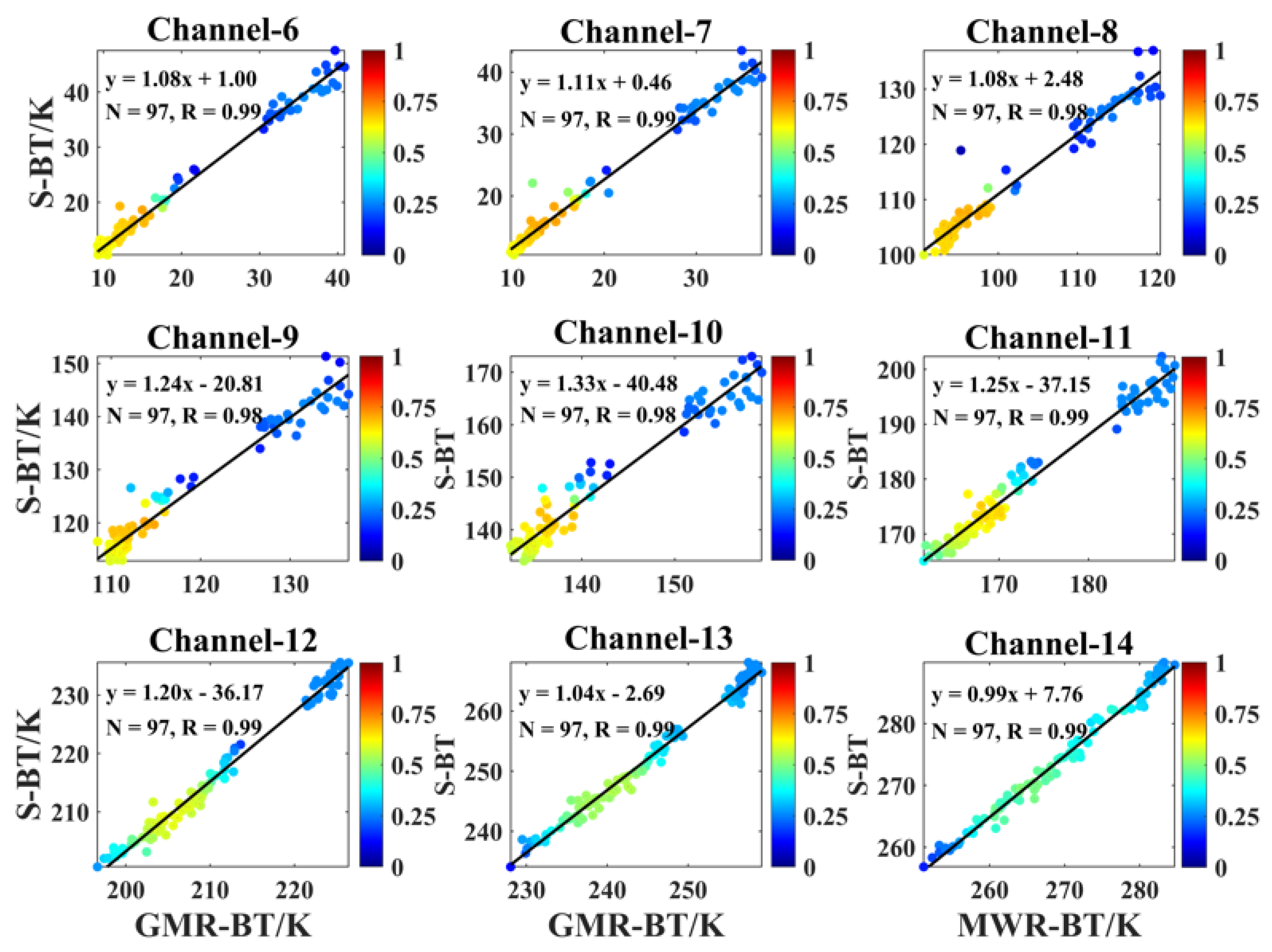
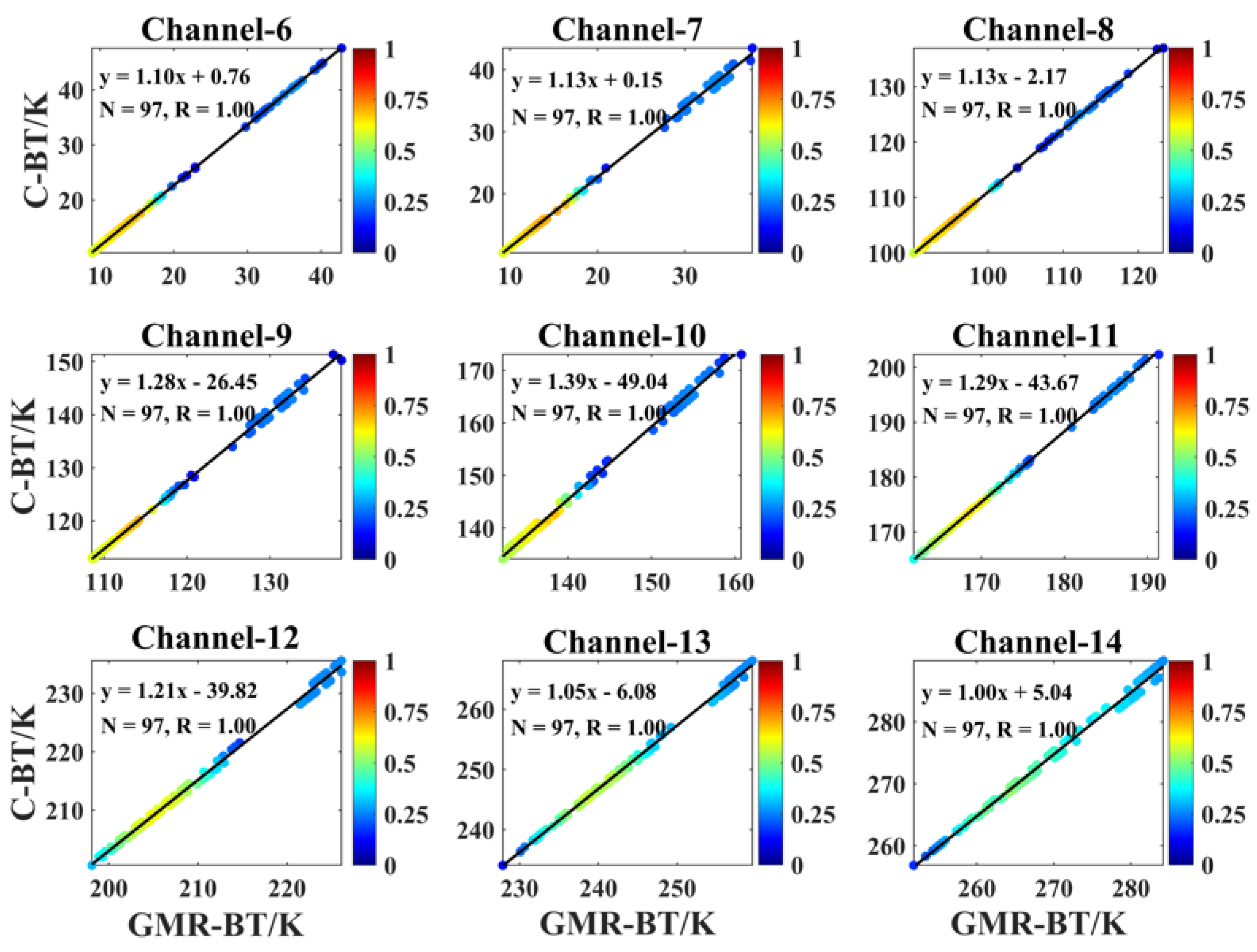
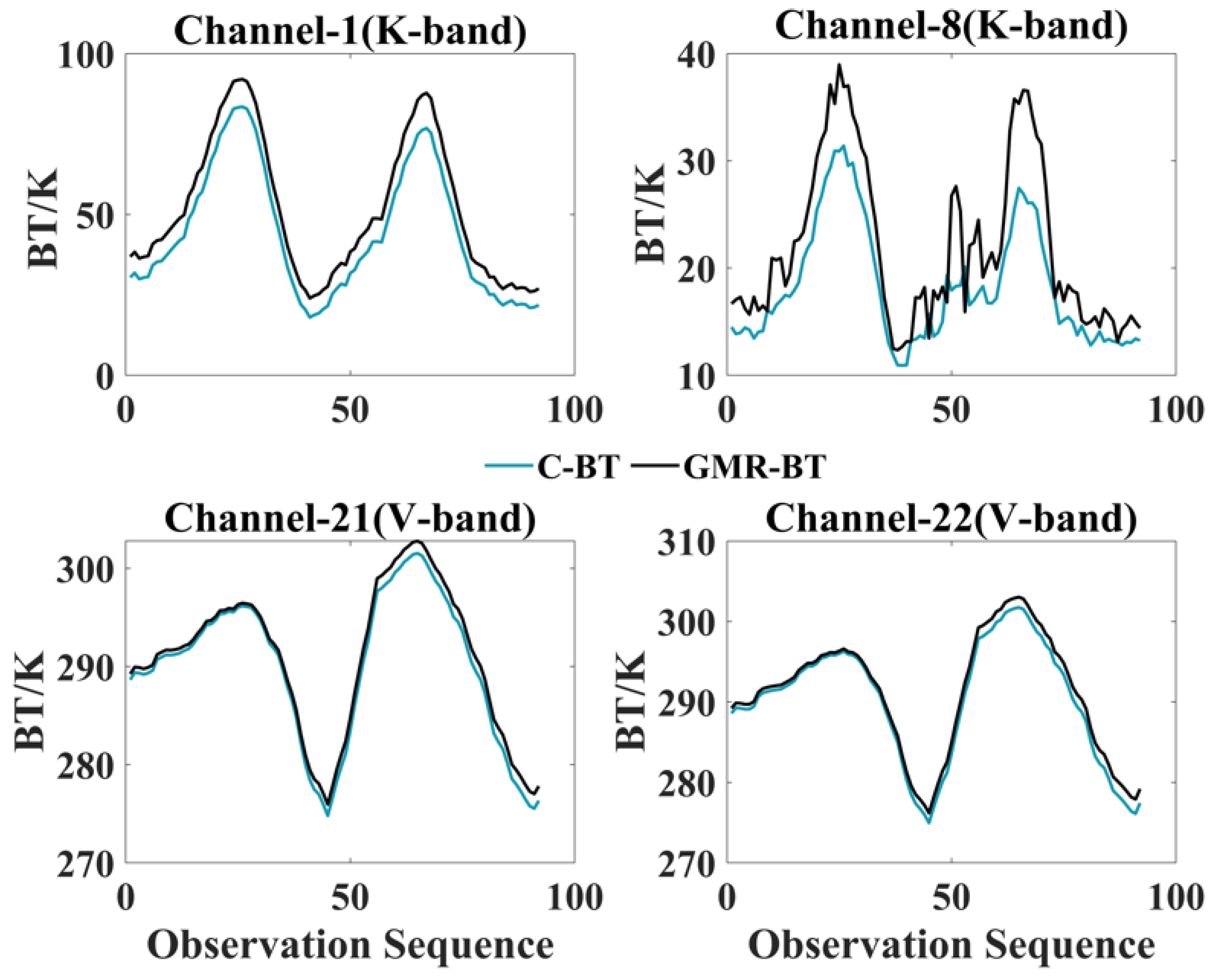
2.5.2. Brightness Temperature Correction

The microwave radiometer measures the actual brightness temperature, and its accuracy significantly influences the precision of the retrieval results. This experiment used sounding data to simulate the brightness temperature during the model training process, while the actual measured brightness temperature was used during the retrieval. The difference between the two caused bias in the retrieval results [25]. Therefore, it was essential to correct the deviation in the simulated brightness temperature values before establishing the retrieval temperature and RH profiles with the actual brightness temperature measured using the GMR. Linear fitting was conducted on the measured and S-BT for each channel based on the sample data (92 sets of data under cloudy conditions and 97 sets of data under clear conditions). The least-squares method was employed to correct the simulated brightness temperature, as follows:

$$\mathrm{Y}=\mathrm{K}\mathrm{X}+\mathrm{B},$$

(6)

$$\mathrm{K}={\displaystyle \frac{\sum \mathrm{x}\mathrm{y}-\mathrm{n}\overline{\mathrm{x}}\overline{\mathrm{y}}}{\sum {\mathrm{x}}^2-\mathrm{n}{\overline{\mathrm{x}}}^2}},$$

(7)

K and B are the slope and intercept in the linear function, where $\mathrm{Y}$ is the corrected simulated brightness temperature (C-BT), $\mathrm{X}$ denotes the BT measured by the GMR (GMR-BT), $\mathrm{n}$ represents the number of sample points, and $\left(\mathrm{x},\mathrm{y}\right)$ denotes GMR-BT and S-BT sample points. The relation between the C-BT and GMR-BT is established in

Table 3. Relation between the measured and simulated brightness temperatures.

Channel Frequency/GHZ	Coefficient K	Coefficient B
22.235	0.96	−3.82
22.500	0.99	−4.95
23.035	0.96	−2.95
23.835	0.96	−3.14
25.000	0.90	−1.91
26.235	0.90	−0.58
28.000	0.90	−0.56
30.000	0.90	−0.43
51.250	0.80	0.37
51.760	0.80	16.91
52.280	0.70	33.18
52.800	0.79	31.18
53.340	0.85	−28.23
53.850	0.90	−1.33
54.400	1.00	−18.53
54.940	1.08	−23.77
55.500	1.00	−9.68
56.020	1.00	−8.48
56.660	1.00	−25.83
57.290	1.05	−16.29
57.960	1.09	−26.05
58.800	1.08	−22.49

.

C-BT was used for neural network model training. GMR-BT was used in the temperature and humidity profile retrieval process.

Figure 1 and Figure 2 show the fitted scatter plots of S-BT, C-BT, and GMR-BT for channels 6–15 of the microwave radiometer. The qualitative analysis of the two plots revealed that the S-BT and GMR-BT exhibited a significant correlation, which was even more pronounced for the C-BT.

Figure 3 and Figure 4 show the variation in the brightness temperature in the K- and V-bands of the GMR at Jinghe Station in Xi’an in 2018. The curve in the figure shows an “M” shape with two peaks, which can be attributable to two reasons. One is that the first half of the “M”-shaped curve is the brightness temperature data at 08:00, and the second half is the brightness temperature data at 20:00 in 2018. The second is that the brightness temperature will peak in summer due to the increase in temperature, enhancing the radiation of water vapor and oxygen molecules, and increasing the brightness temperature values. The qualitative analysis of the two plots showed that the trends of both the C-BT and GMR-BT curves were consistent under both clear and cloudy conditions, indicating that C-BT is able to accurately simulate the microwave radiometer observations of the brightness temperature.

The quantitative analysis shown in Figure 5 revealed that the S-BT errors were significantly higher under cloudy conditions compared with clear conditions. The phenomenon was more evident in the first eight channels of the retrieval water vapor and the first five channels of the retrieval temperature. These channels were more sensitive to the water vapor information contained in the cloud. From a quantitative perspective, the average MAE was 4.14 K under clear conditions and 4.87 K under cloudy conditions. Additionally, the MAE showed a decreasing trend for the first eight channels of retrieval water vapor and the last four channels of retrieval temperature.

2.6. Experimental Methods and Analysis

2.6.1. Retrieval Method

The advantages and disadvantages of four common retrieval methods were compared, as shown in

Table 4. Comparison of the effectiveness of four common retrieval methods.

Retrieval Algorithm	Advantage	Disadvantage
Neural network	Very high precision; Fast computing speed; No modeling required; Algorithmic stability.	Relies on historical data
Kalman filter	Fast computing speed; Error estimation	Relies on historical data; Relies on precision filtering model; Filter divergence.
Genetic algorithm	Monitoring of anomalous changes	Long computation time
Iterative algorithm	Simple to use	Instability

. Compared to the other algorithms, the neural network algorithm is highly precise, runs fast, requires no modeling, and is algorithmically stable.

Neural networks offer substantial advantages in terms of tackling nonlinear problems and have been successfully applied across diverse domains, delivering remarkable outcomes [37,38,39]. Among these, the BPNN has emerged as one of the most widely employed algorithms. First introduced in 1985 by a team of scientists led by Rumelhart [40,41], the BP neural network emulates the response mechanism of neurons in the human brain to external stimuli. This model establishes a multi-layer perceptron and employs the learning mechanisms of forward signal propagation and error backpropagation. Through iterative training, it adeptly constructs intelligent models capable of handling complex nonlinear information. Extensive research in this area has indicated that a single hidden layer in BPNN can obtain the precision of a continuous function [42,43].

2.6.2. Sample Construction

In order to investigate the effect of BPNN in retrieving temperature and RH profiles under clear and cloudy conditions and the effect of adding cloud information on the retrieval of temperature and RH profiles, two sets of experiments were performed, as detailed in this paper. Firstly, the temperature and RH profiles were retrieved under clear conditions; secondly, the temperature and RH profiles were retrieved under cloudy conditions. According to Kolmogorov theory [39], a three-layer neural network with a single hidden layer (with a sufficiently large number of nodes) can approximate any nonlinear continuous function on an arbitrary pre-divided closed set. Therefore, a three-layer BPNN was used in this study to capture the nonlinear relationships between the ground temperature, humidity, pressure, and radiant brightness temperature parameters as well as the atmospheric parameter profiles. The ground temperature, humidity, pressure, and radiant brightness temperature were used as the input parameters, and the atmospheric parameter profiles to be inverted were used as the output parameters.

For clear conditions, the input layer had 25 input nodes including surface temperature, surface relative humidity, surface pressure, and the simulated brightness temperature of the ww channels; for cloudy conditions, cloud information was added to the input layer with 27 input nodes. The output layers included both the temperature and RH profiles of the 83 height layers to be retrieved. The number of nodes in the hidden layer was calculated using the following empirical formula [44,45]:

$$\mathrm{H}=\sqrt{0.4\cdot \mathrm{I}\cdot \mathrm{O}+0.12{\mathrm{O}}^2+2.54\mathrm{I}+0.77\mathrm{O}+0.35}+0.51,$$

(8)

For Equation (8), $\mathrm{I}$ represents the number of nodes in the input layer, $\mathrm{O}$ denotes the number of nodes in the output layer, and $\mathrm{H}$ is the number of nodes in the hidden layer.

For clear conditions, the training dataset included 97 datasets, totaling 10,476 data points while the testing dataset consisted of 17 sets, amounting to 1836 data points. The testing of dataset errors was computed quantitatively, and the four most representative retrieval results were chosen for qualitative analysis. For cloudy conditions, the training dataset consisted of 94 datasets, encompassing 10,340 data points. The testing dataset and analytical approaches remained consistent with those applied to clear conditions.

2.6.3. Sensitivity Experiments of Cloud Information

To analyze the influence of cloud information on retrieval, we performed a test experiment for the sensitivity relating to the uncertainty of clouds. In general, it is considered that low clouds are determined when the cloud-base height is below 2500 m, medium clouds are determined when the cloud-base height is between 2500 m and 6000, and high clouds are determined when the cloud-base height is above 6000 m. In the test, we kept the other parameter fixed, only modifying the cloud-base height or cloud thickness, and then compared the difference between the output atmospheric profiles. The two cases are shown as follows.

Figure 6 and Figure 7 illustrate the impact of cloud information on the temperature profiles (a and b) and the relative humidity profiles (c and d). The initial cloud base or thickness was kept constant while artificially increasing the cloud thickness or cloud-base height incrementally.

Altering the cloud thickness in the presence of low cloud conditions could yield a stable temperature profile. Below 2 km, a marginal rise in relative humidity was observed with the thickening of the cloud layer. Above 8 km, an ascending trend in relative humidity profiles was evident with the augmentation of cloud thickness. Modifying the cloud-base height yielded negligible alterations in the temperature profile below 8 km. Between 8 km and 10 km, a marginal increase was noted in the temperature profile. Beyond 8 km, an elevation in cloud-base height corresponded to reduced relative humidity profiles.

There was no significant alteration in the temperature profiles following the modification of cloud thickness and base height under high cloud conditions. Above 6 km, the cloud thickness increased with the increase in relative humidity profile, while altering the cloud-base height showed no notable changes in relative humidity between 0 and 6 km, with significant but irregular variations above 6 km.

The effects of different cloud-base heights and cloud thicknesses on the temperature profile are illustrated as being insignificant. However, for relative humidity, the modified cloud-base height caused a significant change in the relative humidity on the set cloud-base height, and the peak relative humidity also changed significantly with the set cloud-base height. The modified thickness also significantly increased the relative humidity on the cloud.

3. Results

In Figure 8, four different cases of retrieval results were selected. As can be seen in the figure, the GMR and BPNN retrieval profiles agreed with the Wyoming sounding data. In the overall trend, the temperature decreased gradually with increasing altitude. Above 7.5 km, the three temperature profiles began to show small errors. In Figure 8b–d, temperature inversion occurred at the top of the troposphere (around 10 km), and this phenomenon occurred frequently in the Xi’an area [46]. The heat sources of the atmosphere are solar radiation and ground radiation, and the atmosphere at the top of the troposphere is far from the ground and is less affected by ground radiation but more affected by solar radiation. At this time, the troposphere is influenced by solar radiation, and the temperature inverts and shows an upward trend. In the stratosphere, the atmosphere is mainly affected by solar radiation, and the temperature shows an increasing trend with height. This phenomenon occurs at the junction of the top of the troposphere and the stratosphere due to radiative heating.

Figure 9 shows the fitted scatter plots and error plots under clear conditions, using the radiosonde data of Wyoming as the reference measurements. As can be seen, the retrieval temperature profiles demonstrated a significant fitting relationship with the radiosonde data. The GMR retrieval MAE was 1.7 °C, and the RMSE was 2.2 °C. The BPNN retrieval MAE was 1.3 °C, and the RMSE was 1.9 °C. This shows that the BPNN-coupled MonoRTM is more effective. As shown in Figure 9c,d, the RMSE values of the GMR fluctuated between 1.4 °C and 4.6 °C; the error gradually increased with increasing height, and the minimum and maximum values were obtained at around 0 km and 10 km, respectively. At 7.8 km, the RMSE value of the GMR started slightly lower than that of the BPNN, and the reason for this phenomenon is complicated; for example, there was still an error between C-BT and GMR-BT. However, since the difference between these two was less than 0.5 °C above 7.8 km, it did not affect the accuracy of the overall comparison of the temperature profile retrieval. The RMSE value of the BPNN retrieval fluctuated between 0.7 °C and 4.6 °C; the error gradually increased with increasing height, and the minimum and maximum values were obtained at 0.8 km and 9.75 km, respectively. In general, the trend of the MAE plot was the same as that of the RMSE plot. At the altitude of 0–7.25 km, the MAE value of BPNN was lower than that of the GMR, and at the altitude of 7.25–10 km, the two errors were close to each other.

Figure 10 shows the four typical cases of the RH profile retrieval comparison plots under clear conditions. At an altitude of 0~2 km, both the BPNN and GMR were consistent with the radiosonde data, and the relative humidity decreased and then increased near the ground, with a trough at about 0.5 km and a peak at about 2 km. The reason for this phenomenon was the presence of humidity inversion at the ground [47]. At an altitude of 2~10 km, the RH profiles of GMR retrieval started to deviate from the radiosonde data, and the maximum error were approximately 15%, 40%, 50%, and 20%, respectively, in the four graphs shown in Figure 10a–d. The retrieval RH profiles of the BPNN-coupled MonoRTM still demonstrated an accurately fitting relationship with the radiosonde data, with maximum errors of approximately 7%, 11%, 16%, and 20%, respectively.

The scatter plots fitted to the radiosonde data and error plots of RH profiles under clear conditions are shown in Figure 11. In Figure 11a,b, the retrieval errors of the GMR can be seen as follows: the MAE was 11.4% and RMSE was 15.0%. The retrieval errors of the BPNN were as follows: the MAE was 7.7% and RMSE was 11.7%. Compared with the GMR, the retrieval method of the BPNN-coupled MonoRTM improved the retrieval accuracy of the RH profiles to some extent. As shown in Figure 11c,d, at a height of 0$~$1 km, it can be seen that the retrieval error of the GMR increased and then decreased, and the error was the smallest around 0 km, with an RMSE of 4.8$\%$ and MAE of 4.0%; meanwhile, the retrieval error of BPNN decreased and then increased, and there was a trough at 0.5 km, with an RMSE at 3.6% and a MAE at 2.8%. At an altitude of 1$~$10 km, the retrieval accuracy of the GMR retrieved RH profiles was the lowest, with the RMSE at 3.6% and MAE at 2.8%. The GMR error and the BPNN error were closest at 4.25 km and 1.85 km, respectively, as shown in Figure 11c,d. After exceeding the height, the error of the BPNN-coupled MonoRTM showed a decreasing tendency; meanwhile, the retrieval error of the GMR started to rise and then decreased and reached the maximum at 6.75 km. The RMSE and MAE of GMR were 27.3% and 26.4%, respectively, and both decreased gradually from 6.75 km to 10 km. The maximum values of the RMSE of the GMR and MAE of GMR were obtained at 6.75 km. The differences in the RMSE and MAE between the GMR and BPNN were 12.5% and 15.5%, respectively.

Figure 12 shows four typical examples under cloudy conditions for the three retrieval methods including BPNN, BPNN (cloud), and GMR using the Wyoming sounding data as reference measurements. By analyzing Figure 12, it can be seen that the results of the three retrieval methods were consistent with the sounding data, indicating that the retrieval of temperature profiles was relatively stable and that the temperature profiles were insensitive to the cloud information; additionally, it also verified the conclusions of the cloud information sensitivity experiment.

The conclusions of the above experiments confirmed the superiority of the BPNN-coupled MonoRTM compared with the GMR. Therefore, in the subsequent experiments of error analysis with clouds, only the specific effects of cloud information on the temperature and RH profiles retrieval were explored. In a typical case, the GMR retrieval profiles were still used as a control group.

Figure 13 illustrates the fitted scatter plots and error plots of the temperature profiles before and after the addition of cloud information, using the sounding data as reference measurements. Figure 13a,b shows that in the cloudy samples, the MAE (BPNN) was 2.6 °C, RMSE (BPNN) was 2.4 °C, MAE (BPNN (cloud)) was 1.9 °C, RMSE (BPNN (cloud)) was 1.7 °C, and the accuracy of the temperature profiles was improved to some extent after the addition of the cloud information. As shown in Figure 13c,d, the addition of cloud information significantly improved the accuracy of the temperature profiles at an altitude of 0~10 km. Without the addition of cloud information, the RMSE and MAE of the BPNN retrieval fluctuated between 1.6 °C~4.2 °C and 1.7 °C~4.7 °C, respectively, and the minimum and maximum values were obtained at 0.65 km and 10 km, respectively. However, with the addition of cloud information, the RMSE and MAE fluctuated between 1.0 °C~3.6 °C and 1.1 °C~3.9 °C, respectively, and the minimum and maximum values were the same as those without the cloud information. At an altitude of 0~3.5 km, the changes in error before and after the addition of cloud information were small, and the error became larger at an altitude of 3.5 km~10 km. At around 7.75 km, the accuracy of the temperature profiles received the greatest improvement, and the RMSE and MAE errors both decreased around 1.0 °C after the addition of cloud information.

Figure 14 illustrates the plot of the RH profiles for the BPNN, BPNN (cloud), and the GMR retrievals under cloudy conditions with the sounding data as reference measurements. In Figure 14, it can be seen that the three retrieval methods could better approach the sounding data at an altitude of 0~2 km. However, the RH profiles of BPNN retrieval and GMR retrieval showed a large error relative to that of BPNN (cloud) retrieval at an altitude of 2~10 km. Taking Figure 14a as an example, at a height around 6.25 km, the errors of GMR retrieval, BPNN, and BPNN (cloud) retrieval with the sounding data reached their maximum, which were 37.9%, 33.2%, and 18.6% respectively. This shows that the inclusion of cloud information improved the accuracy of the RH profiles, especially within the height of the cloud layer. The water vapor content of clouds was assumed to be one of the main factors affecting the RH profile retrieval, and the RH of the sounding data increased sharply within the height of the cloud layer. The cloud types shown in Figure 14a,c,d should be noted as single-layer clouds, and in Figure 14a,d, the GMR and BPNN retrieval had the largest errors in the range of cloud-base heights, whereas in Figure 14c, such a situation did not occur. After several sets of experiments, the effect of thin clouds on the RH profiles was identified as being lower than that of thick clouds. This speculation can also be verified in the retrieval results relating to double-layer clouds, as shown in Figure 14b, where the first layer of clouds belonged to medium and thin clouds, the second layer of clouds belonged to medium and thick clouds, and the maximum point of error between the sounding data and the GMR and the BPNN occurred at around 4.5 km (the second layer of clouds).

Figure 15 shows the scatter plots fitted to the sounding data and error plots of the RH profiles under cloudy conditions. The retrieval errors can be seen in Figure 15a,b: the MAE (BPNN) was 13.1%, RMSE (BPNN) was 16.6%, MAE (BPNN (cloud) was 12.2%, and RMSE (BPNN (cloud) was 15.0%. The inclusion of cloud information reduced both the sample MAE and RMSE. The analysis in Figure 15c shows that the RMSE of BPNN and BPNN (cloud) retrieved RH profiles fluctuated in the ranges of 6.2~27.8% and 4.6~19.9%, respectively, with the minimum and maximum values of the errors at the ground and at around 7 km. At the altitude of 0~1 km, the error of BPNN was slightly lower than that of BPNN (cloud); meanwhile, the errors of BPNN were higher than that of BPNN (cloud) in the altitude range of 2~10 km. Above 1 km, the inclusion of cloud information significantly improved the accuracy of the RH profiles.

4. Conclusions

This study focused on combining active and passive remote sensing to extensively analyze the specific influence of cloud information on the temperature and RH profile retrieval and further improve the accuracy of atmospheric temperature and RH profile retrieval. Three types of data (Huai’an sounding data, GMR data, and MWCR data) from the same site under sunny and cloudy conditions at Jinghe Station in Xi’an in 2018 were selected to carry out the experiment. The main conclusions can be summarized as follows:

(1)

The MonoRTM simulated brightness temperature had significantly higher errors under cloudy conditions than clear conditions. This phenomenon was more significant in the water vapor channel and the first five channels of the retrieval temperature, and it can be speculated that these channels may be more sensitive to the water vapor content of the cloud information compared to the other channels.

(2)

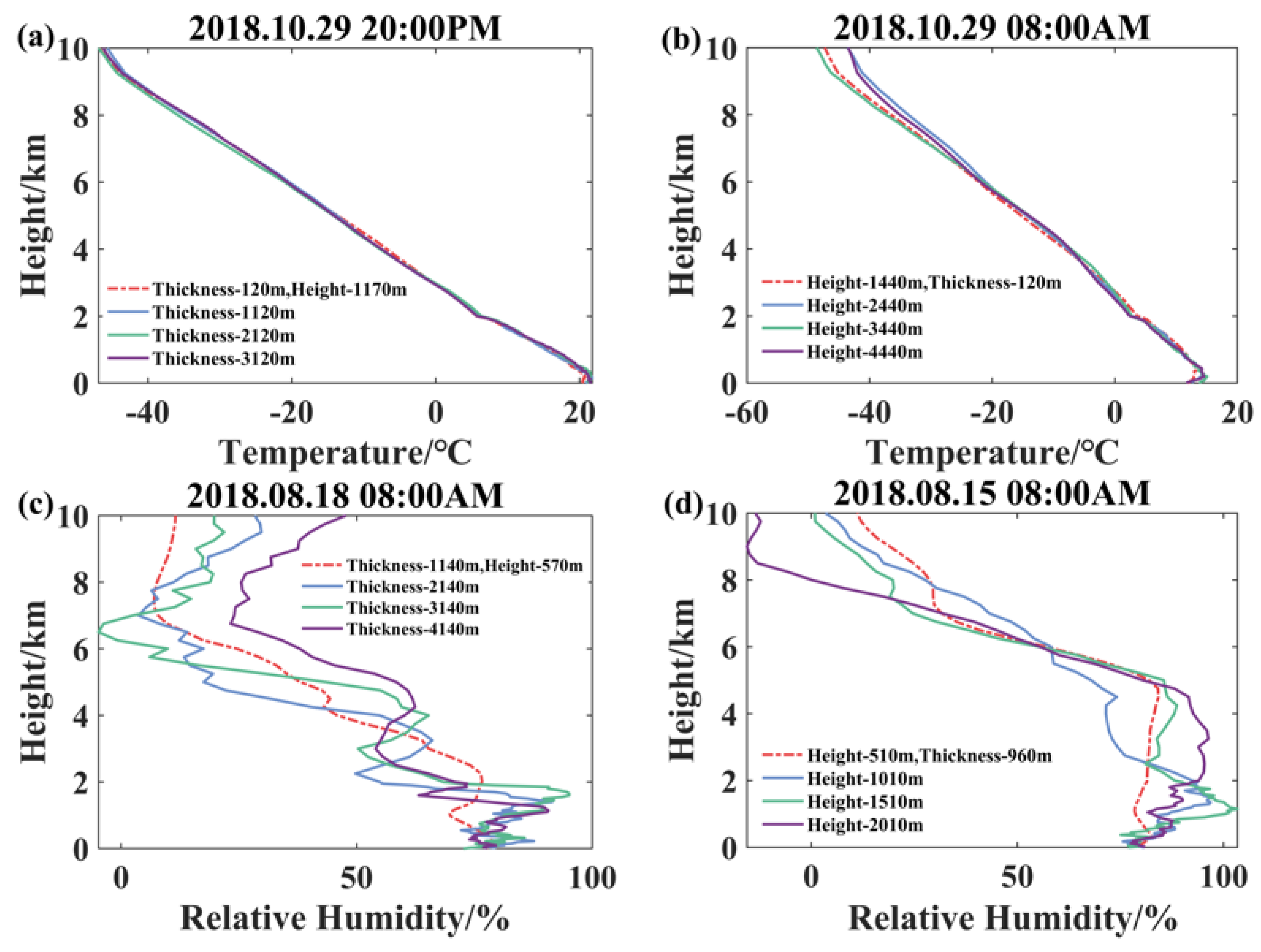
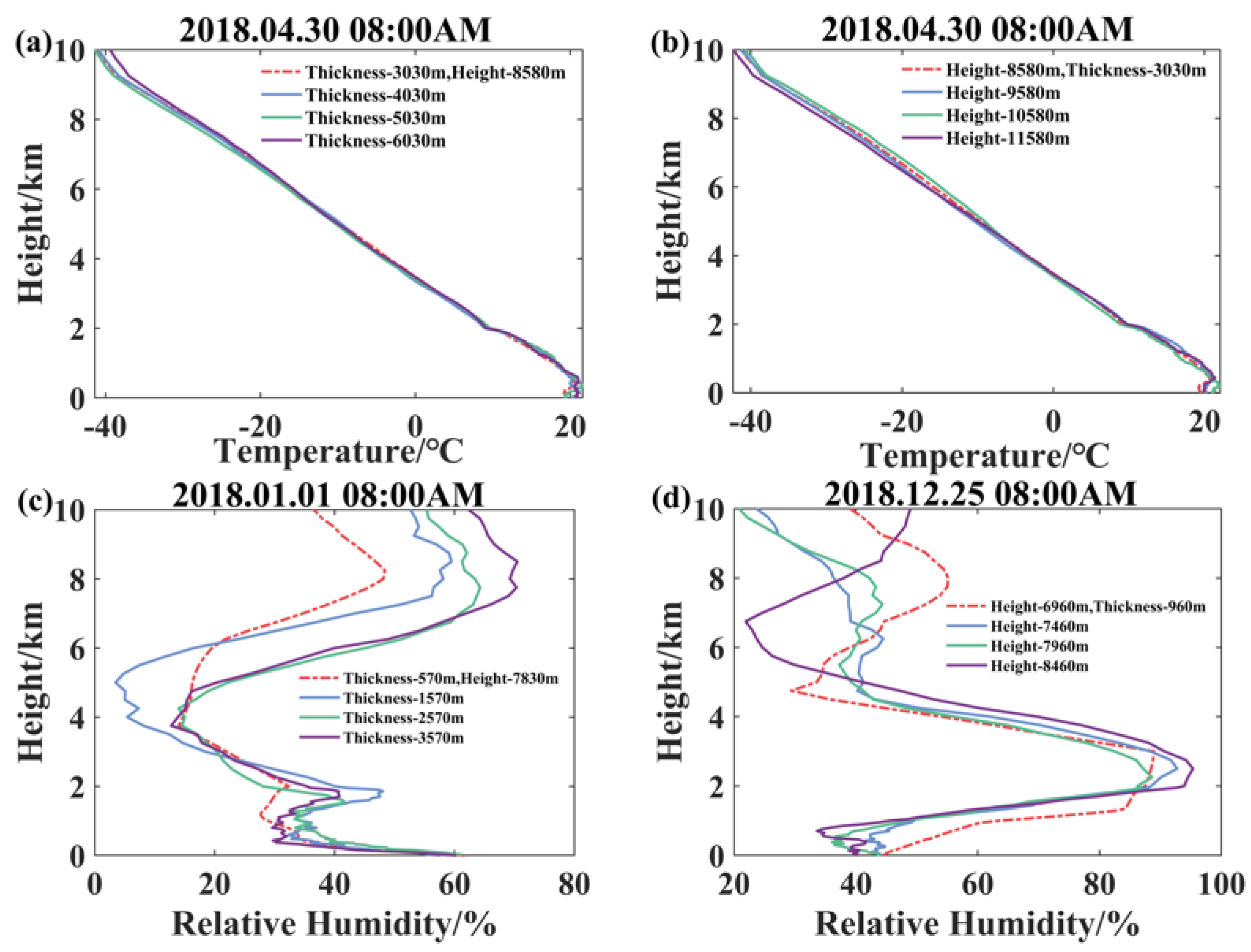
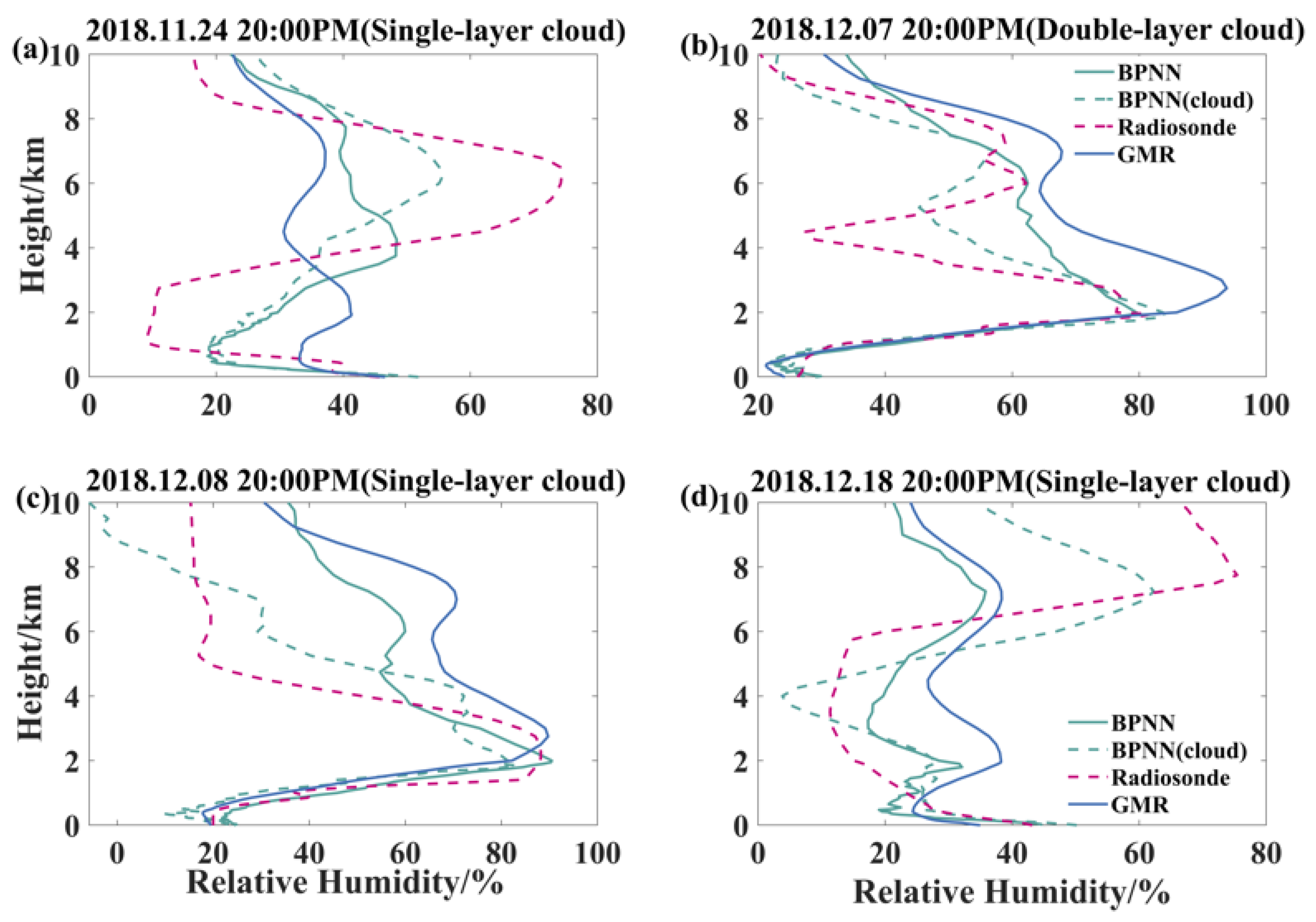
The effect of different cloud-base heights and cloud thicknesses on the temperature profiles was not significant. However, for the relative humidity profiles, altering the cloud-base height and thickness led to significant changes in the relative humidity and its peak. Altering the thickness led to a significant increase in the relative humidity within the cloud layer. For low cloud conditions, when changing the cloud-base height or cloud thickness, 2 km is the critical height layer for significant differences in RH profiles; for high cloud conditions, the critical height layer is 4 km.

(3)

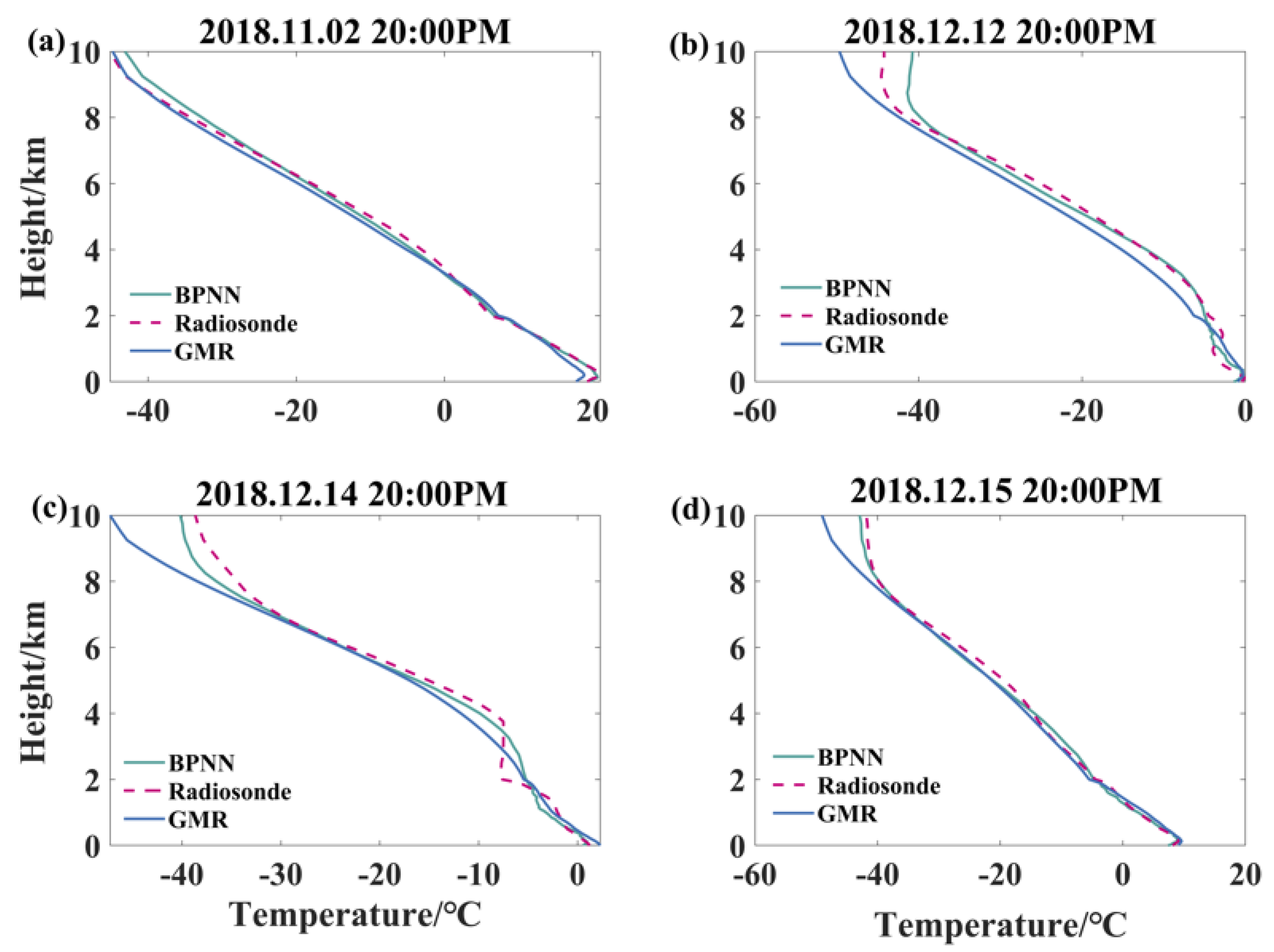
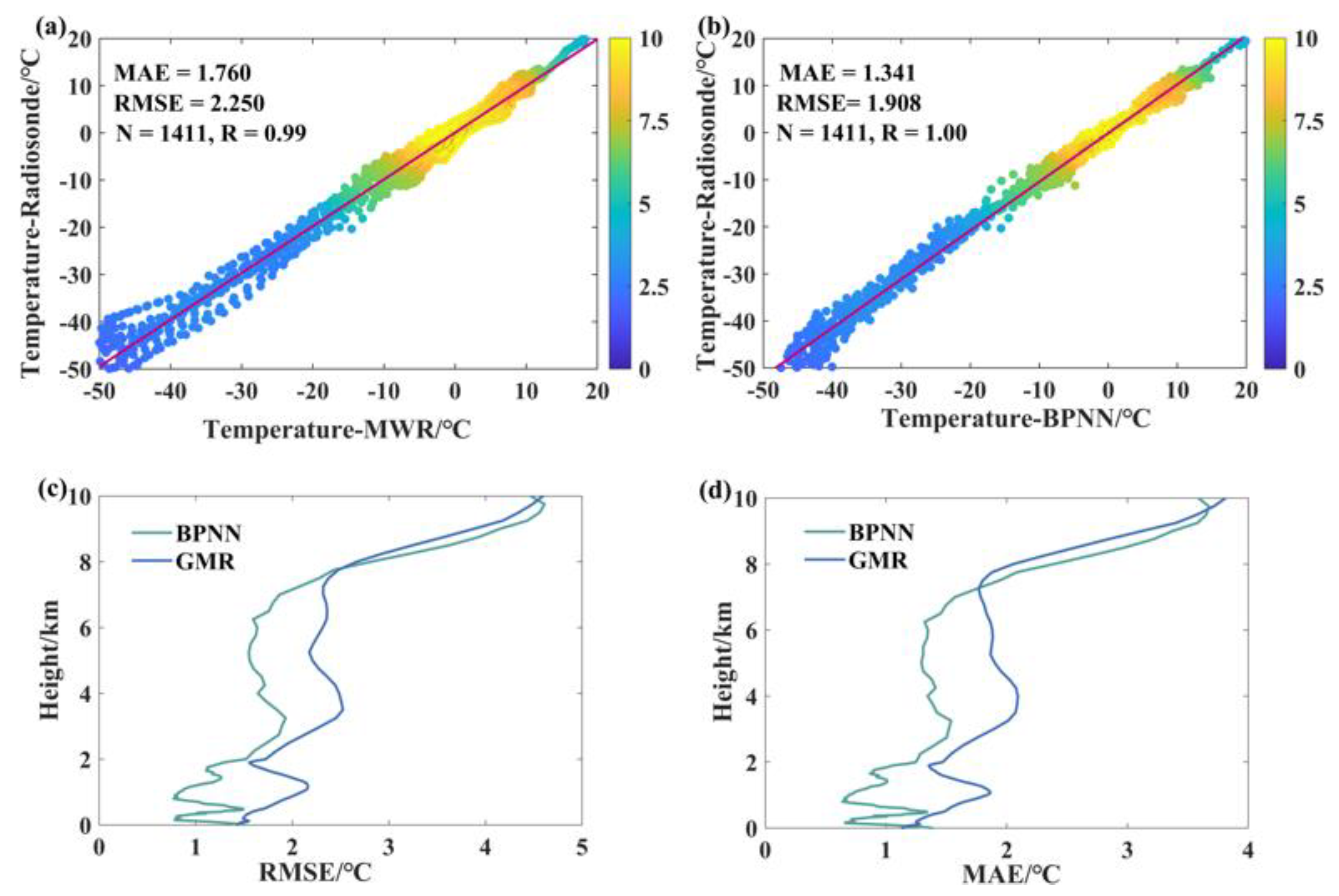
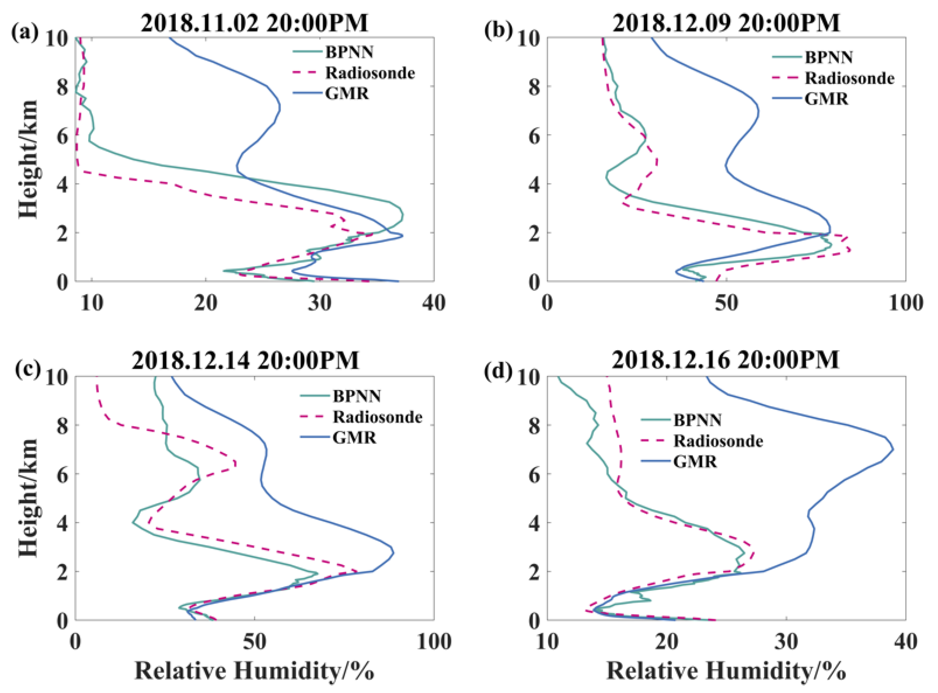
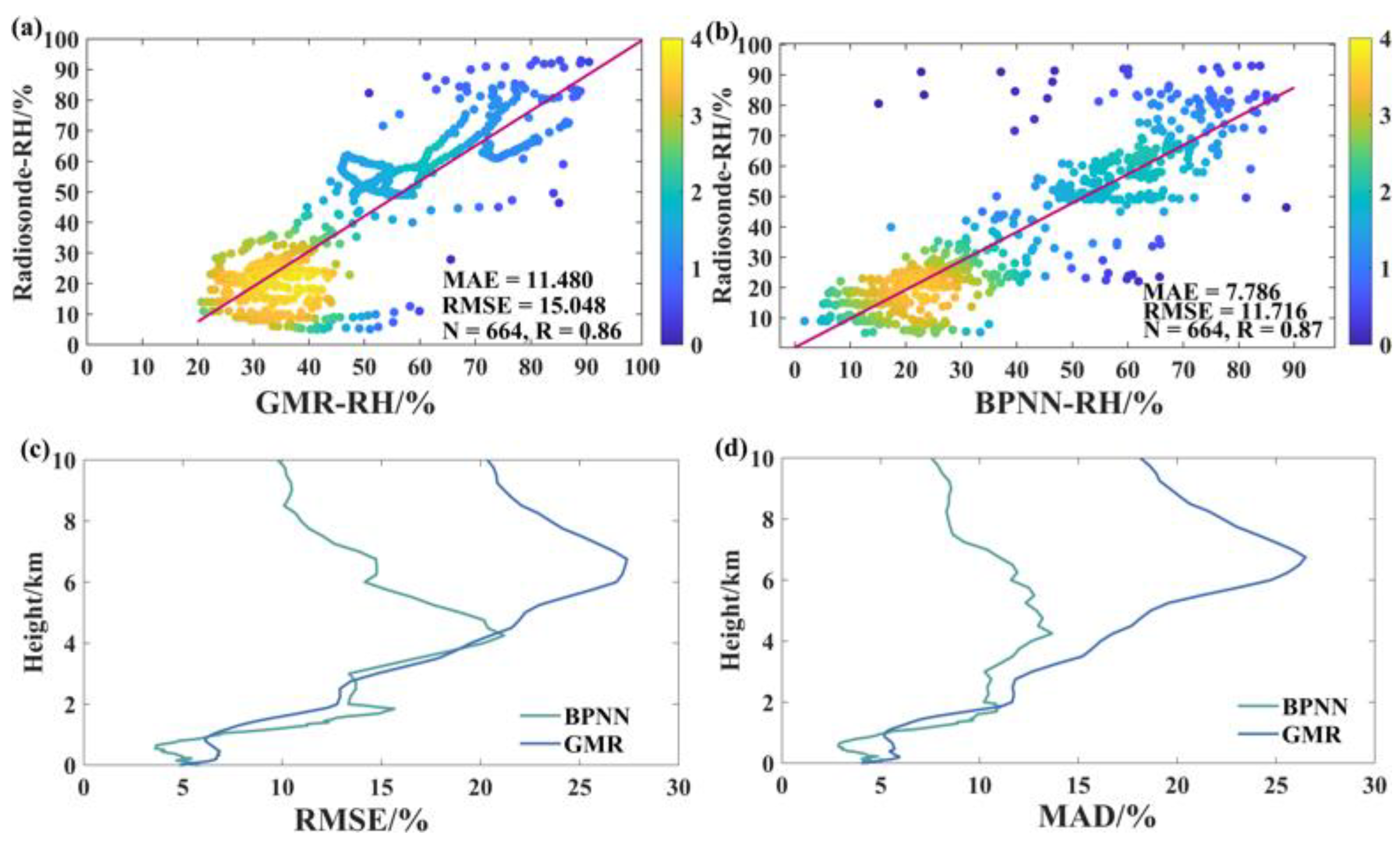
For temperature profile retrieval under clear conditions, both the BPNN and GMR retrievals demonstrated better performance. Overall, the errors of the temperature profiles increased with an increase in altitude, and the error of GMR retrieval was slightly higher than that of BPNN retrieval. However, for RH profile retrieval, the BPNN retrieval of the RH profiles was significantly better than GMR retrieval. This is related to the fact that some channels of the microwave radiometer are more sensitive to water vapor information.

(4)

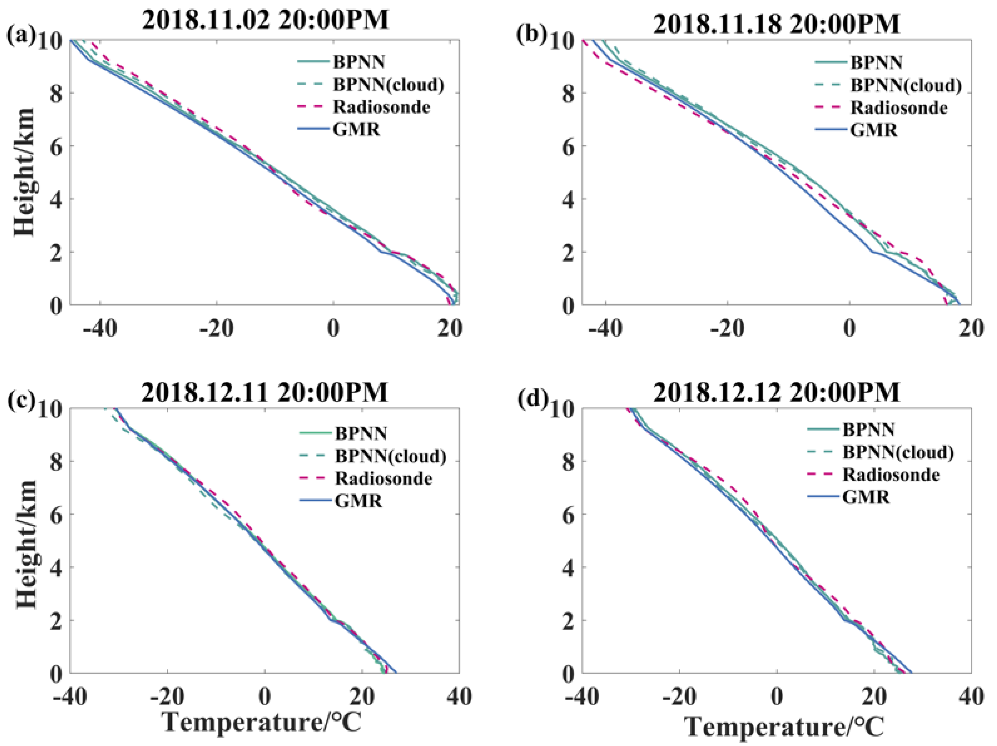
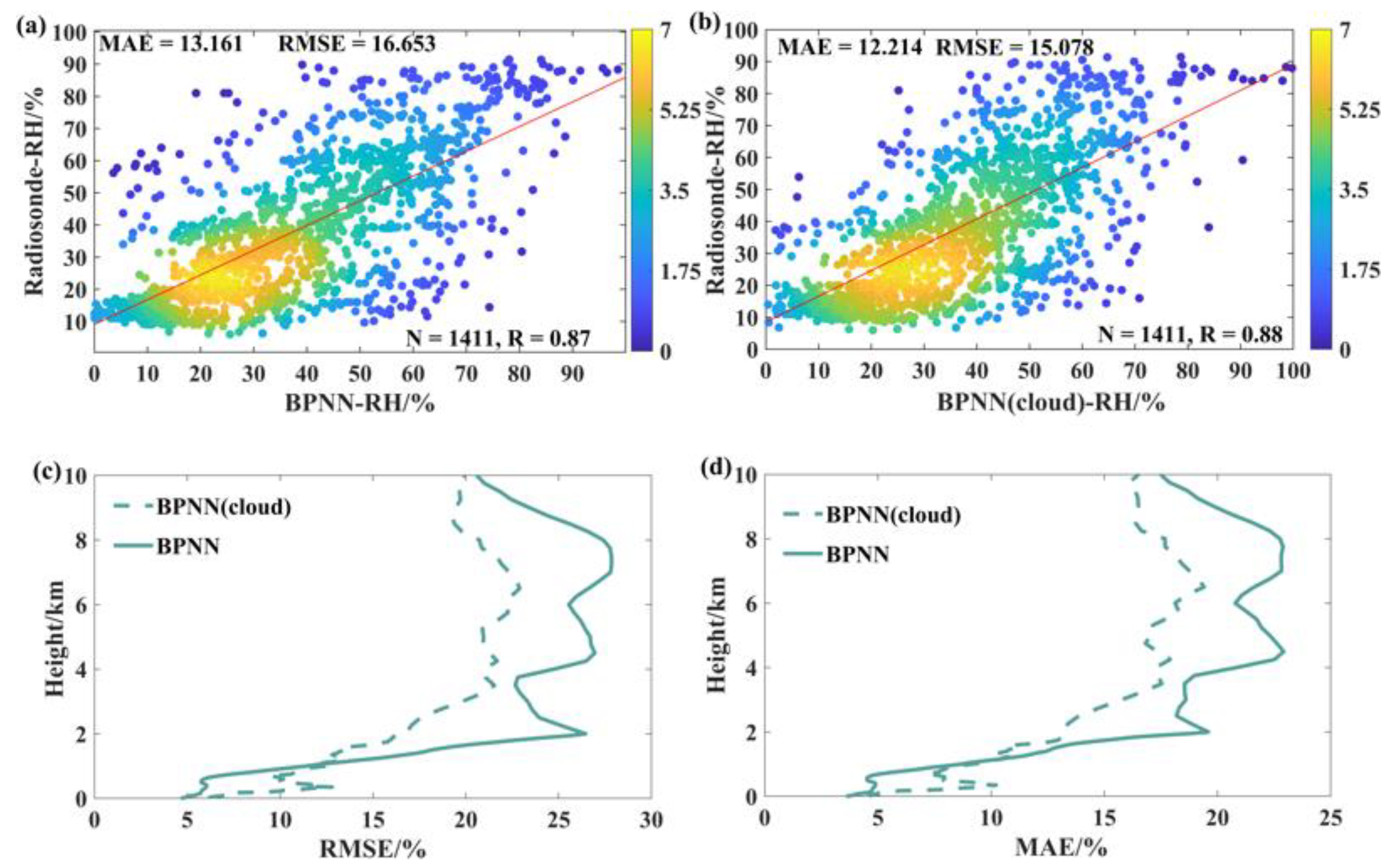
For temperature and RH profile retrieval under cloudy conditions, it can be seen from the typical cases that the temperature profile retrieval was basically stable; in the height ranges of single-layer and double-layer clouds, the sounding relative humidity increased sharply due to the influence of water vapor in the clouds. The comparison experiments revealed that cloud thickness was the main factor affecting the relative humidity profiles. For thick clouds, the GMR and BPNN retrieval method without cloud information demonstrated the largest errors. With the cloud information, the accuracy of the BPNN retrieval was improved above 2 km, especially in thick clouds. The retrieval temperature and relative humidity profiles with the cloud information were better than the retrieval without the cloud information. The retrieval temperature and RH profiles with the cloud information were closer to the sounding data compared with the retrieval without the cloud information. From a quantitative point of view, the errors of the retrieval of temperature and relative humidity profiles slightly improved with the addition of cloud information.

This study employed active and passive observations combined with remote sensing retrieval to extensively investigate the specific influence of cloud information on temperature and RH profile retrieval. The retrieval accuracy for the atmospheric temperature and RH profiles was further improved, providing the necessary data for numerical weather prediction and global climate assessments; moreover, it also provides a certain reference value for the study of soil temperature and RH retrieval using GMR as well as for fire monitoring.

In the future, we will obtain richer cloud information data and perform an in-depth investigation of cloud thickness, cloud-base height, and the effect of cloud shape on temperature and RH profile retrieval and boundary layer retrieval.

References

1. Li, H.; Cheng, J.; Zhang, Q.; Zheng, B.; Zhang, Y.; Zheng, G.; He, K. Rapid Transition in Winter Aerosol Composition in Beijing from 2014 to 2017: Response to Clean Air Actions. Atmos. Chem. Phys. 2019, 19, 11485–11499. [Google Scholar] [CrossRef]
2. Temimi, M. On the Analysis of Ground-Based Microwave Radiometer Data during Fog Conditions. Atmos. Res. 2020, 231, 104652. [Google Scholar] [CrossRef]
3. Yan, X.; Liang, C.; Jiang, Y.; Luo, N.; Zang, Z.; Li, Z. A Deep Learning Approach to Improve the Retrieval of Temperature and Humidity Profiles from a Ground-Based Microwave Radiometer. IEEE Trans. Geosci. Remote Sens. 2020, 58, 8427–8437. [Google Scholar] [CrossRef]
4. Hu, J.; Bao, Y.; Liu, J.; Liu, H.; Petropoulos, G.P.; Katsafados, P.; Zhu, L.; Cai, X. Temperature and Relative Humidity Profile Retrieval from Fengyun-3D/HIRAS in the Arctic Region. Remote Sens. 2021, 13, 1884. [Google Scholar] [CrossRef]
5. Zhou, Z.; Kou, X.; Zhao, S.; Jiang, L. A New Method to Inverse Soil Moisture Based on Thermal Infrared and Passive Microwave Remote Sensing. In Land Surface Remote Sensing II; Jackson, T.J., Chen, J.M., Gong, P., Liang, S., Eds.; SPIE: Beijing, China, 2014; p. 926026. [Google Scholar]
6. Laroche, S.; Sarrazin, R. Impact of Radiosonde Balloon Drift on Numerical Weather Prediction and Verification. Weather Forecast. 2013, 28, 772–782. [Google Scholar] [CrossRef]
7. Seidel, D.J.; Sun, B.; Pettey, M.; Reale, A. Global Radiosonde Balloon Drift Statistics. J. Geophys. Res. 2011, 116, D07102. [Google Scholar] [CrossRef]
8. Seidel, D.J.; Randel, W.J. Variability and Trends in the Global Tropopause Estimated from Radiosonde Data. J. Geophys. Res. 2006, 111, 2006JD007363. [Google Scholar] [CrossRef]
9. Seidel, D.J.; Ao, C.O.; Li, K. Estimating Climatological Planetary Boundary Layer Heights from Radiosonde Observations: Comparison of Methods and Uncertainty Analysis. J. Geophys. Res. 2010, 115, D16113. [Google Scholar] [CrossRef]
10. Qi, Y.; Fan, S.; Li, B.; Mao, J.; Lin, D. Assimilation of Ground-Based Microwave Radiometer on Heavy Rainfall Forecast in Beijing. Atmosphere 2022, 13, 74. [Google Scholar] [CrossRef]
11. Cao, Y.; Shi, B.; Zhao, X.; Yang, T.; Min, J. Direct Assimilation of Ground-Based Microwave Radiometer Clear-Sky Radiance Data and Its Impact on the Forecast of Heavy Rainfall. Remote Sens. 2023, 15, 4314. [Google Scholar] [CrossRef]
12. Shi, J.; Du, Y.; Du, J.; Jiang, L.; Chai, L.; Mao, K.; Xu, P.; Ni, W.; Xiong, C.; Liu, Q.; et al. Progresses on Microwave Remote Sensing of Land Surface Parameters. Sci. China Earth Sci. 2012, 55, 1052–1078. [Google Scholar] [CrossRef]
13. Payne, V.H.; Mlawer, E.J.; Cady-Pereira, K.E.; Moncet, J.-L. Water Vapor Continuum Absorption in the Microwave. IEEE Trans. Geosci. Remote Sens. 2011, 49, 2194–2208. [Google Scholar] [CrossRef]
14. Loehnert, U.; Maier, O. Operational Profiling of Temperature Using Ground-Based Microwave Radiometry at Payerne: Prospects and Challenges. Atmos. Meas. Tech. 2012, 5, 1121–1134. [Google Scholar] [CrossRef]
15. Candlish, L.M.; Raddatz, R.L.; Asplin, M.G.; Barber, D.G. Atmospheric Temperature and Absolute Humidity Profiles over the Beaufort Sea and Amundsen Gulf from a Microwave Radiometer. J. Atmos. Ocean. Technol. 2012, 29, 1182–1201. [Google Scholar] [CrossRef]
16. Sánchez, J.L.; Posada, R.; García-Ortega, E.; López, L.; Marcos, J.L. A Method to Improve the Accuracy of Continuous Measuring of Vertical Profiles of Temperature and Water Vapor Density by Means of a Ground-Based Microwave Radiometer. Atmos. Res. 2013, 122, 43–54. [Google Scholar] [CrossRef]
17. Ware, R.; Cimini, D.; Campos, E.; Giuliani, G.; Albers, S.; Nelson, M.; Koch, S.E.; Joe, P.; Cober, S. Thermodynamic and Liquid Profiling during the 2010 Winter Olympics. Atmos. Res. 2013, 132–133, 278–290. [Google Scholar] [CrossRef]
18. Wei, J.; Shi, Y.; Ren, Y.; Li, Q.; Qiao, Z.; Cao, J.; Ayantobo, O.O.; Yin, J.; Wang, G. Application of Ground-Based Microwave Radiometer in Retrieving Meteorological Characteristics of Tibet Plateau. Remote Sens. 2021, 13, 2527. [Google Scholar] [CrossRef]
19. Askne, J.; Westwater, E. A Review of Ground-Based Remote Sensing of Temperature and Moisture by Passive Microwave Radiometers. IEEE Trans. Geosci. Remote Sens. 1986, GE-24, 340–352. [Google Scholar] [CrossRef]
20. Cimini, D.; Hewison, T.J.; Martin, L.; Güldner, J.; Marzano, F.S. Temperature and Humidity Profile Retrievals from Ground-Based Microwave Radiometers during TUC. Meteorol. Z. 2006, 15, 45–56. [Google Scholar] [CrossRef]
21. Bianco, L.; Cimini, D.; Marzano, F.S.; Ware, R. Combining Microwave Radiometer and Wind Profiler Radar Measurements for High-Resolution Atmospheric Humidity Profiling. J. Atmos. Ocean. Technol. 2005, 22, 949–965. [Google Scholar] [CrossRef]
22. Klaus, V.; Bianco, L.; Gaffard, C.; Matabuena, M.; Hewison, T.J. Combining UHF Radar Wind Profiler and Microwave Radiometer for the Estimation of Atmospheric Humidity Profiles. Meteorol. Z. 2006, 15, 87–97. [Google Scholar] [CrossRef]
23. Liljegren, J.C.; Clothiaux, E.E.; Mace, G.G.; Kato, S.; Dong, X. A New Retrieval for Cloud Liquid Water Path Using a Ground-Based Microwave Radiometer and Measurements of Cloud Temperature. J. Geophys. Res. 2001, 106, 14485–14500. [Google Scholar] [CrossRef]
24. Chan, P.W. Performance and Application of a Multi-Wavelength, Ground-Based Microwave Radiometer in Intense Convective Weather. Meteorol. Z. 2009, 18, 253–265. [Google Scholar] [CrossRef]
25. Ren, Y.J. Inversion of Temperature and Humidity Profile of Microwave Radiometer Based on BP Network. Intell. Autom. Soft Comput. 2021, 29, 741–755. [Google Scholar]
26. Frate, F.D.; Schiavon, G. A Combined Natural Orthogonal Functions/Neural Network Technique for the Radiometric Estimation of Atmospheric Profiles. Radio Sci. 1998, 33, 405–410. [Google Scholar] [CrossRef]
27. Solheim, F.; Godwin, J.R.; Westwater, E.R.; Han, Y.; Keihm, S.J.; Marsh, K.; Ware, R. Radiometric Profiling of Temperature, Water Vapor and Cloud Liquid Water Using Various Inversion Methods. Radio Sci. 1998, 33, 393–404. [Google Scholar] [CrossRef]
28. Li, Q.; Wei, M.; Wang, Z.; Jiang, S.; Chu, Y. Improving the Retrieval of Cloudy Atmospheric Profiles from Brightness Temperatures Observed with a Ground-Based Microwave Radiometer. Atmosphere 2021, 12, 648. [Google Scholar] [CrossRef]
29. Turner, D.D.; Clough, S.A.; Liljegren, J.C.; Clothiaux, E.E.; Cady-Pereira, K.E.; Gaustad, K.L. Retrieving Liquid Wat0er Path and Precipitable Water Vapor From the Atmospheric Radiation Measurement (ARM) Microwave Radiometers. IEEE Trans. Geosci. Remote Sens. 2007, 45, 3680–3690. [Google Scholar] [CrossRef]
30. Clough, S.A.; Shephard, M.W.; Mlawer, E.J.; Delamere, J.S.; Iacono, M.J.; Cady-Pereira, K.; Boukabara, S.; Brown, P.D. Atmospheric Radiative Transfer Modeling: A Summary of the AER Codes. J. Quant. Spectrosc. Radiat. Transf. 2005, 91, 233–244. [Google Scholar] [CrossRef]
31. Fixsen, D.J. The Temperature of the Cosmic Microwave Background. Astrophys. J. 2009, 707, 916–920. [Google Scholar] [CrossRef]
32. Zhao, B.; Fu, Q.; Du, J.; Hu, C.; Li, H. Microwave Remote-Sensing of Atmospheric Property and Weather Process. Sci. China Ser. B-Chem. Life Sci. Earth Sci. 1991, 34, 352–362. [Google Scholar]
33. Pan, Y. Analysis on the Solar Influence to Brightness Temperatures Observed with a Ground-Based Microwave Radiometer. J. Atmos. Sol.-Terr. Phys. 2021, 222, 105725. [Google Scholar] [CrossRef]
34. Che, Y.; Ma, S.; Xing, F.; Li, S.; Dai, Y. An Improvement of the Retrieval of Temperature and Relative Humidity Profiles from a Combination of Active and Passive Remote Sensing. Meteorol. Atmos. Phys. 2019, 131, 681–695. [Google Scholar] [CrossRef]
35. Cimini, D.; Marzano, F.S.; Ciotti, P.; Westwater, E.R.; Kehim, S.J.; Han, Y. Empirical Evaluation of Four Microwave Radiative Forward Models Based on Ground-Based Radiometer Data near 20 and 30 GHz. In Proceedings of the IGARSS 2003: IEEE International Geoscience and Remote Sensing Symposium, Vols I—VII, Proceedings: Learning from Earth’s Shapes and Sizes, Toulouse, France,, 21–25 July 2003; IEEE: New York, NY, USA, 2003; pp. 1502–1504. [Google Scholar]
36. Tan, H.; Mao, J.; Chen, H.; Chan, P.W.; Wu, D.; Li, F.; Deng, T. A Study of a Retrieval Method for Temperature and Humidity Profiles from Microwave Radiometer Observations Based on Principal Component Analysis and Stepwise Regression. J. Atmos. Ocean. Technol. 2011, 28, 378–389. [Google Scholar] [CrossRef]
37. Hu, H.-Y.; Lee, Y.-C.; Yen, T.-M.; Tsai, C.-H. Using BPNN and DEMATEL to Modify Importance–Performance Analysis Model—A Study of the Computer Industry. Expert Syst. Appl. 2009, 36, 9969–9979. [Google Scholar] [CrossRef]
38. Ghose, D.K.; Panda, S.S.; Swain, P.C. Prediction of Water Table Depth in Western Region, Orissa Using BPNN and RBFN Neural Networks. J. Hydrol. 2010, 394, 296–304. [Google Scholar] [CrossRef]
39. Bashir, T.; Haoyong, C.; Tahir, M.F.; Liqiang, Z. Short Term Electricity Load Forecasting Using Hybrid Prophet-LSTM Model Optimized by BPNN. Energy Rep. 2022, 8, 1678–1686. [Google Scholar] [CrossRef]
40. Rumelhart, D.E.; Hinton, G.E.; Williams, R.J. Learning Representations by Back-Propagating Errors. Nature 1986, 323, 533–536. [Google Scholar] [CrossRef]
41. Dai, H.; MacBeth, C. Effects of Learning Parameters on Learning Procedure and Performance of a BPNN. Neural Netw. 1997, 10, 1505–1521. [Google Scholar] [CrossRef]
42. Yu, W.; Xu, X.; Jin, S.; Ma, Y.; Liu, B.; Gong, W. BP Neural Network Retrieval for Remote Sensing Atmospheric Profile of Ground-Based Microwave Radiometer. IEEE Geosci. Remote Sens. Lett. 2022, 19, 4502105. [Google Scholar] [CrossRef]
43. Xi, C.; Qi-feng, L.; Quan, Z. 0–10 km Temperature and Humidity Profiles Retrieval from Ground-Based Microwave Radiometer. J. Trop. Meteorol. 2018, 24, 243–252. [Google Scholar]
44. Wanas, N.; Auda, G.; Kamel, M.S.; Karray, F. On the Optimal Number of Hidden Nodes in a Neural Network. In Proceedings of the Conference Proceedings. IEEE Canadian Conference on Electrical and Computer Engineering (Cat. No.98TH8341), Kingston, ON, Canada, 25–28 May 1998; Volume 2, pp. 918–921. [Google Scholar]
45. Cai, G.-W.; Fang, Z.; Chen, Y.-F. Estimating the Number of Hidden Nodes of the Single-Hidden-Layer Feedforward Neural Networks. In Proceedings of the 2019 15th International Conference on Computational Intelligence and Security (CIS), Macao, China, 13–16 December 2019; pp. 172–176. [Google Scholar]
46. Li, Y.; Yan, J.; Sui, X. Tropospheric Temperature Inversion over Central China. Atmos. Res. 2012, 116, 105–115. [Google Scholar] [CrossRef]
47. Zhou, X.; Zhang, C.; Li, Y.; Sun, J.; Chen, Z.; Li, L. Concurrence of Temperature and Humidity Inversions in Winter in Qingdao, China. Geophys. Res. Lett. 2024, 51, e2024GL108350. [Google Scholar] [CrossRef]
Figure 1. The fitting graph of S-BT and GMR-BT for channels 6–14 under clear conditions.
Atmosphere 15 01064 g001
Figure 2. The fitting graph of C-BT and GMR-BT for channels 6–14 under clear conditions.
Atmosphere 15 01064 g002
Figure 3. A comparison of C-BT and GMR-BT in the K-band and V-band under clear conditions.
Atmosphere 15 01064 g003
Figure 4. A comparison of C-BT and GMR-BT in the K-band and V-band under cloudy conditions.
Atmosphere 15 01064 g004
Figure 5. The MAE comparison of C-BT and GMR-BT for Xi’an’s Jinghe Station in 2018.
Atmosphere 15 01064 g005
Figure 6. The impact of cloud information on the temperature (a,b) and relative humidity (c,d) profiles of low cloud conditions.
Atmosphere 15 01064 g006
Figure 7. The impact of cloud information on the temperature (a,b) and relative humidity (c,d) profiles of high cloud conditions.
Atmosphere 15 01064 g007
Figure 8. A comparison between the temperature profiles generated using the BPNN retrieval models, the GMR product, and the radiosonde under clear conditions at (a) 20:00 (UTC + 8) on 2 November 2018; (b) 20:00 (UTC + 8) on 12 December 2018; (c) 20:00 (UTC + 8) on 14 December 2018; and (d) 20:00 (UTC + 8) on 15 December 2018.
Atmosphere 15 01064 g008
Figure 9. The radiosonde data were used as reference measurements to compare the BPNN retrieval models and the GMR product under clear conditions for (a) the GMR and radiosonde data temperature profile scatter plots; (b) the BPNN and radiosonde data temperature profile scatter plots; (c) the RMSE of the temperature profiles; and (d) the MAE of the temperature profiles.
Atmosphere 15 01064 g009
Figure 10. A comparison between the relative humidity profiles generated using the BPNN retrieval model, the GMR product, and the radiosonde under clear conditions at (a) 20:00 (UTC + 8) on 2 November 2018; (b) 20:00 (UTC + 8) on 9 December 2018; (c) 20:00 (UTC + 8) on 14 December 2018; and (d) 20:00 (UTC + 8) on 16 December 2018.
Atmosphere 15 01064 g010
Figure 11. Using radiosonde data as reference measurements, a comparison of the BPNN retrieval models and the GMR product under clear conditions for (a) the GMR and radiosonde data relative humidity profile scatter plots; (b) the BPNN and radiosonde data relative humidity profile scatter plots; (c) the RMSE of the relative humidity profiles; and (d) the MAE of the relative humidity profiles.
Atmosphere 15 01064 g011
Figure 12. A comparison between the temperature profiles generated using the BPNN and BPNN (cloud) retrieval models, the GMR product, and the radiosonde under cloudy conditions at (a) 20:00 (UTC + 8) on 2 November 2018; (b) 20:00 (UTC + 8) on 18 November 2018; (c) 20:00 (UTC + 8) on 11 December 2018; and (d) 20:00 (UTC + 8) on 12 December 2018.
Atmosphere 15 01064 g012
Figure 13. Using radiosonde data as reference measurements, a comparison of the BPNN and BPNN (cloud) retrieval models under cloudy conditions for (a) the BPNN and radiosonde data temperature profile scatter plot; (b) the BPNN (cloud) and radiosonde data temperature profile scatter plots; (c) the RMSE of the temperature profiles; and (d) the MAE of the temperature profiles.
Atmosphere 15 01064 g013
Figure 14. A comparison between the relative humidity profiles generated using the BPNN and BPNN (cloud) retrieval models, the GMR product, and the radiosonde under cloudy conditions at (a) 20:00 (UTC + 8) on 24 November 2018 (single-layer cloud: cloud-base height: 5190 m; cloud thickness: 2100 m); (b) 20:00 (UTC + 8) on 7 December 2018 (double-layer cloud: cloud-base height: 2850(330) m; cloud thickness: 5970(1560) m); (c) 20:00 (UTC + 8) on 8 December 2018 (single-layer cloud: cloud-base height: 1170 m; cloud thickness: 540 m); and (d) 20:00 (UTC + 8) on 18 December 2018 (single-layer cloud: cloud-base height: 6240 m; cloud thickness: 3450 m).
Atmosphere 15 01064 g014
Figure 15. Using radiosonde data as reference measurements, a comparison of the BPNN and BPNN (cloud) retrieval models under cloudy conditions for (a) the BPNN and radiosonde data relative humidity profile scatter plots; (b) the BPNN (cloud) and radiosonde data relative humidity profile scatter plots; (c) the RMSE of the relative humidity profiles; and (d) the MAE of the relative humidity profiles.
Atmosphere 15 01064 g015