Abstract
Developing short-term forecasting models for global atmospheric temperature and wind in near space is crucial for understanding atmospheric dynamics and supporting human activities in this region. While numerical models have been extensively developed, deep learning techniques have recently shown promise in improving atmospheric forecasting accuracy. In this study, convolutional long short-term memory (ConvLSTM) and convolutional gated recurrent unit (ConvGRU) neural networks were applied to build for short-term global-scale forecasting model of atmospheric temperature and wind in near space based on the MERRA-2 reanalysis dataset from 2010–2022. The model results showed that the ConvGRU model outperforms the ConvLSTM model in the short-term forecast results. The ConvGRU model achieved a root mean square error in the first three hours of approximately 1.8 K for temperature predictions, and errors of 4.2 m/s and 3.8 m/s for eastward and northward wind predictions on all 72 isobaric surfaces. Specifically, at a higher altitude (on the 1.65 Pa isobaric surface, approximately 70 km above sea level), the ConvGRU model achieved a RMSE of about 2.85 K for temperature predictions, and 5.67 m/s and 5.17 m/s for eastward and northward wind. This finding is significantly meaningful for short-term temperature and wind forecasts in near space and for exploring the physical mechanisms related to temperature and wind variations in this region.
1. Introduction
Establishing reliable short-term forecasting models can enhance human understanding of the near-space atmosphere and provide support for human activities [1]. Near-space, characterized by its thin atmosphere, experiences significant temperature and wind variations. These strong fluctuations not only affect the environmental adaptability of high-speed aircraft but also influence the aircraft’s flight trajectories and attitude control, posing a threat to the safety of high-speed vehicles [2]. Reliable forecasting of atmospheric temperature and winds in the near-space will facilitate pre-flight assessments, in-flight trajectory predictions, and post-mission environmental evaluations for aircraft [2], thereby safeguarding human activities in the near-space. Moreover, as a transition zone from the lower to the upper atmosphere, forecasting atmospheric temperature and winds in the near space will aid in understanding the interaction mechanisms between these atmospheric layers and the characteristics of atmospheric circulation changes [1,3].
The forecast range for the near-space environment is positioned between meteorological forecasting and space weather forecasting. The near-space environment usually refers to the atmospheric environment in the MLT region (for mesosphere and lower thermosphere) in 20–100 km. There are two methods for predicting the near-space environment: numerical forecasting and statistical forecasting. Numerical forecasting attempts to establish global prediction models to achieve forecasting outcomes, whereas statistical forecasting relies predominantly on regional near-space environmental detection data, employing statistical analysis models for regional forecasts. In the domain of numerical forecasting, years of development have led to the maturation of models such as the HWM series wind field model [4], the NRLMSISE-00 empirical model [5], WACCM-X 2.0 [6], and the U.S. Navy’s global numerical forecasting model NOGAPS-ALPHA (NOGAPS-Advanced Level Physics and High Altitude) [7]. These models can forecast atmospheric temperature and wind fields from the ground to near-space altitudes on a global scale. However, numerical models are influenced by calculable models, initial fields, boundary conditions, and parameterization schemes, which introduce errors. Consequently, forecast data from numerical models often exhibit systematic biases compared to actual observations [8]. In terms of statistical forecasting, Roney J A. [9] studied the wind field at an altitude range of 18–30 km in the near-space to ensure the safe operation of high-altitude aircraft. They established a statistical forecasting model based on observation data from Akon, OH, USA, and White Sands, NM, USA. Liu T. [10] explored the AR (Autoregressive) model based on continuous detection data from single stations in near space. Chen et al. [11] predict regional near-space wind fields using the ERA5 dataset. In the exploration of near-space environment forecasts discussed above, the approach of employing statistical routes for environmental forecasting has been based on either single-site or small regional spatial scales, lacking exploration into global-scale near-space environment forecasts.
In recent years, with the rapid development of computer science and artificial intelligence, statistical methods for global-scale environmental forecasting based on deep learning have gradually been applied to the meteorological forecasting field [12]. Weather prediction models trained using deep learning methods, such as WF-UNet [13], ClimaX [14], GraphCast [15], and Pangu-Weather [16], have improved the real-time accuracy of weather predictions. Notably, the Pangu model’s accuracy in predicting extreme weather has surpassed that of NWP methods for the first time [16]. Inspired by the integration of weather forecasting and artificial intelligence, deep learning methods have also been extended to the near-space environment forecasting field. Biao Chen et al. [17] constructed LSTM and BiLSTM deep learning networks to develop a near-space short-term (48 h) atmospheric temperature forecasting model by applying deep learning to the ERA-5 dataset single-point temperature values at 20–50 km altitude from 1991 to 2000. The model’s forecast accuracy in December reached 0.4371 K (RMSE). However, his study was based on a single-site for forecasting. This paper selects the recently applied ConvLSTM [18] and ConvGRU [19] neural learning networks in the meteorological forecast domain to explore a short-term global-scale near-space environment forecast model. To our knowledge, no team has yet modeled the MERRA-2 reanalysis dataset using convolutional neural networks to perform short-term global-scale forecasts of the near-space environment.
The Introduction section primarily discusses the significance of short-term forecasts in the near-space atmospheric temperature and wind. Motivated by the current popularity of utilizing deep learning for atmospheric forecasting, this chapter proposes the idea of applying deep learning techniques to global-scale, short-term forecasts in the near space. The Data Sources and Preprocessing section and Methodology section detail the dataset used in this study along with the deep learning methods tailored for it, and describe the deep learning neural network that was developed. The Discussion section presents the main forecasting results, analyzing the trained model’s temporal scale prediction accuracy, detailed comparisons between two models, prediction accuracy across different altitudes, and accuracy along latitudinal variations. The Conclusion section sums up the four results and puts forward several aspects that needed improvement which could lay the foundation for subsequent research.
2. Data Sources and Preprocessing
2.1. Data Source
MERRA-2 is NASA’s latest generation of high spatial and temporal resolution global atmospheric reanalysis data. The input Observation of MERRA-2 conclude Conventional Observations, Satellite Observations of Wind and Satellite Observations of Mass [20]. MERRA-2 successfully utilizes the global observing system over the modern era, exploiting the information content contained therein to the fullest extent of the system’s capability. The advantages of MERRA-2 include: it utilizes real-time atmospheric temperature data acquired by the Microwave Limb Sensor (MLS) on the MODIS Aura satellite. The improved calibration coefficients provided by MLS data have achieved better atmospheric correction results in polar regions. Bosilovich et al. [21] found that the MERRA-2 data are close to the observation results, and its temporal discontinuity or spurious trends are small. Duo C et al. found that the MERRA2 dataset is an ideal high-resolution wind field [22] and temperature [23] reanalysis data for the Tibetan Plateau and its surrounding areas. As a result, the temperature and wind field data from MERRA-2 are highly accurate and reliable.
Our study employs the MERRA-2 temperature and wind field products, which offer a spatial resolution of 1.9 × 2.5 degrees and a temporal resolution of three hours, referred to as 3-hourly MERRA2. These products are structured over 72 isobaric surfaces. The data can be accessed at: https://rda.ucar.edu/datasets/ds313.3/dataaccess/# (accessed on 5 December 2023). For this study, data from the years 2010 to 2020 were selected for training, data from 2021 for cross-validation, and data from 2022 for testing.
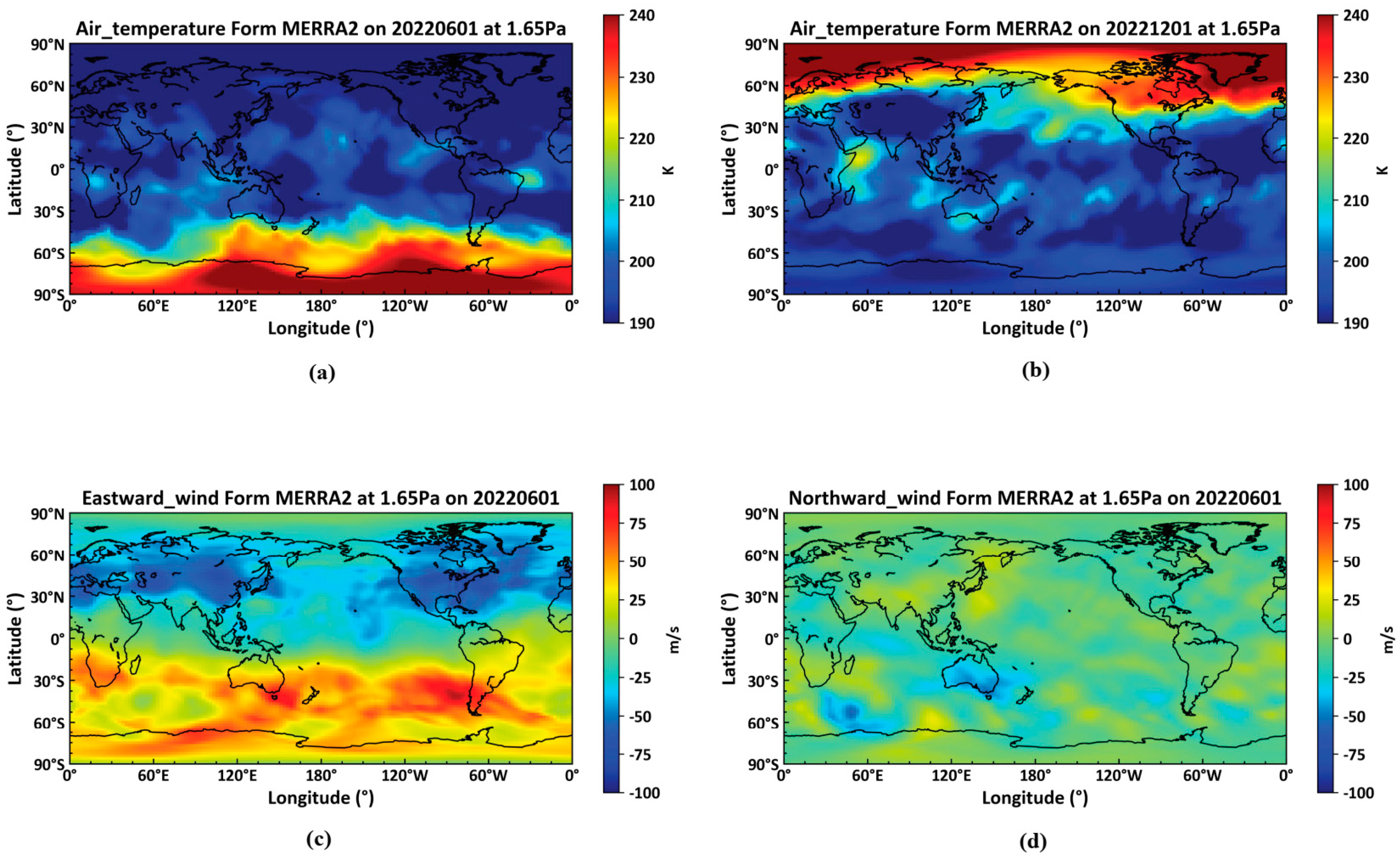
The Figure 1 below displays temperature profiles and horizontal winds at a height of 1.65 Pa from the MERRA2 reanalysis dataset, captured between 9 AM and 12 PM.
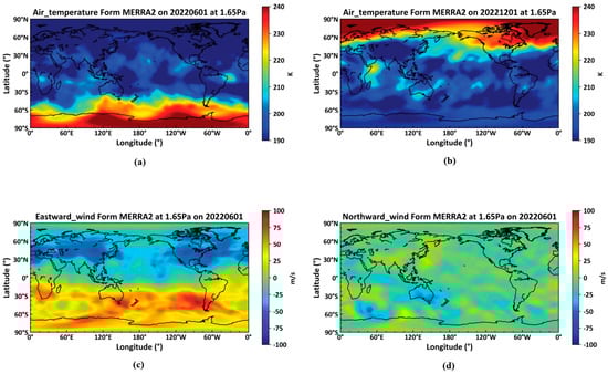
Figure 1.
The results from the MERRA2 reanalysis dataset at a height of 1.65 Pa on 1 June 2022. (a): temperature at 9:00 on 1 June 2022; (b): temperature at 9:00 on 1 December 2022; (c): eastward wind at 9:00 on 1 December 2022; (d): northward wind at 9:00 on 1 December 2022.
2.2. Data Preprocessing
In utilizing recurrent neural networks for predictive modeling, data normalization is typically a crucial step to ensure the stability of both model training and performance.
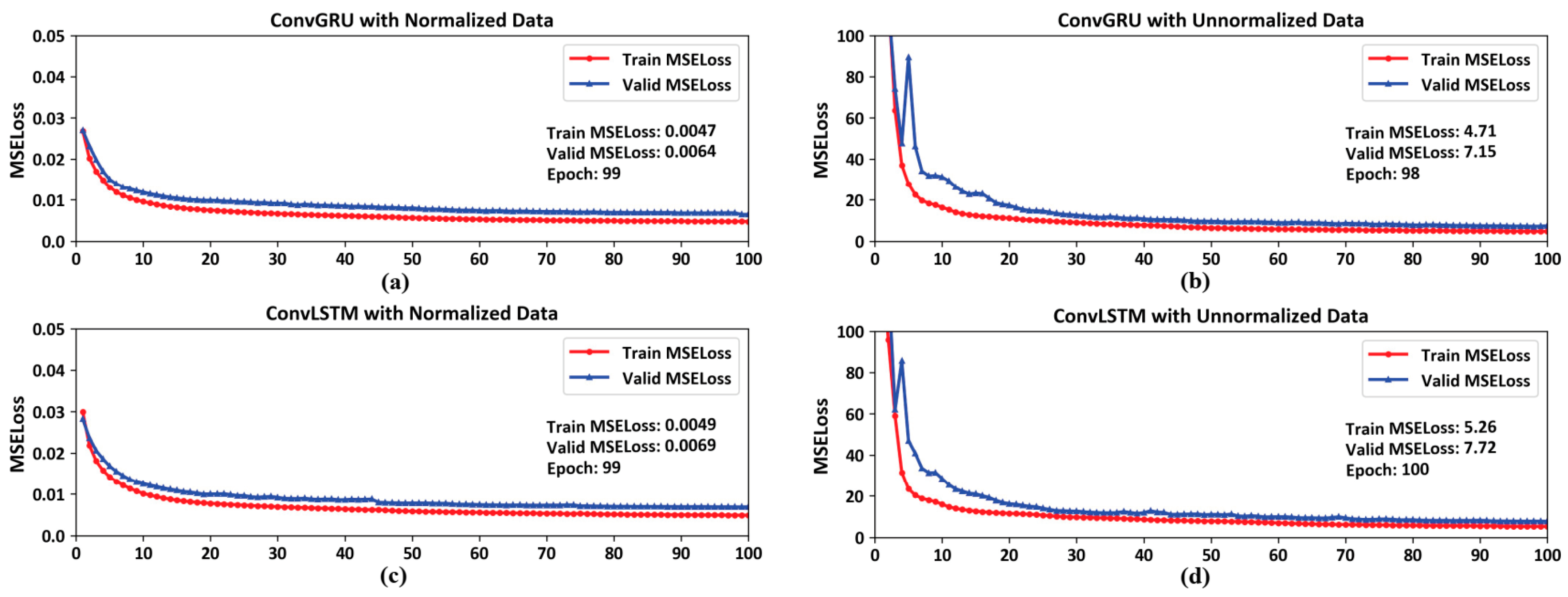
Our study conducts training modeling on standardized and non-standardized temperature data for a period of 10 years across 72 isobaric surface levels, and performs cross-validation with one year of data. It is observed that standardized data allows for quicker convergence during training, and prevents sudden spikes in validation MSELoss in Figure 2. Preprocessing the data can reduce the impact of outliers and data noise on the training process, thereby avoiding large fluctuations in the gradient descent curve. Usually, occurrences of sudden spikes in MSELoss can lead to non-convergence of the model [24].
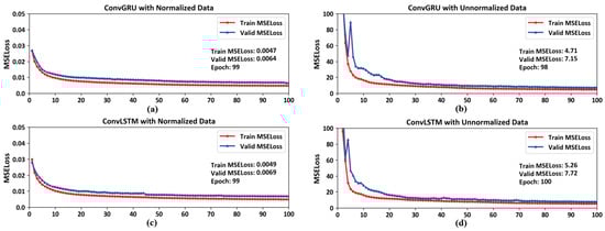
Figure 2.
The MSELoss curves during the training of ConvGRU and ConvLSTM. (a): The MSELoss curves during the training of ConvGRU with normalized data; (b): The MSELoss curves during the training of ConvGRU with unnormalized data; (c): The MSELoss curves during the training of ConvLSTM with normalized data; (d): The MSELoss curves during the training of ConvLSTM with unnormalized data.
The purpose of standardization is to transform data into a standard normal distribution with a mean of zero and a standard deviation of one. This aids in accelerating model convergence and enhancing model performance. In our study, the daily data are treated as a collection, from which the mean and standard deviation are computed.
Our study computes the mean and standard deviation for the daily data, treating it as a unified dataset. Each data point is standardized by subtracting the mean of the dataset and then dividing by its standard deviation as Equation (1):
Here, represents the original input data, denotes the mean of the dataset, and signifies the standard deviation of the dataset.
The output data are standardized using the same formula, employing the mean and standard deviation of the input dataset.
3. Methodology
In the domain of spatiotemporal sequence forecasting, Long Short-Term Memory (LSTM) and Gated Recurrent Unit (GRU) networks represent significant advances within the realm of Recurrent Neural Networks (RNNs). Extensions such as ConvLSTM and ConvGRU have enhanced these traditional models by replacing the fully connected operations in standard RNN units with convolutional operations, thereby enabling the network to process spatiotemporal data more effectively. Shi et al. were the pioneers in employing the ConvLSTM architecture to address the challenge of rainfall forecasting. They constructed an end-to-end trainable model for short-term precipitation forecasting and empirically demonstrated that ConvLSTM outperforms traditional LSTM in capturing spatiotemporal relationships [18]. Kim et al. developed a model using ConvLSTM to predict rainfall amounts from weather radar data. Their experimental findings indicated that a two-layer ConvLSTM model reduced the Root Mean Square Error (RMSE) by 23.0% compared to linear regression [25]. Given the substantial number of parameters in ConvLSTM, which poses a barrier to training, Shi et al. further proposed the ConvGRU model to address this issue. Experimental results showed that it performs better and is easier to train.
Our study targets the spatiotemporal resolution of the MERRA2 dataset and constructs two deep-learning networks, ConvLSTM and ConGRU. Below are the construction methods for both networks.
3.1. Design of Neural Networks
3.1.1. ConvLSTM
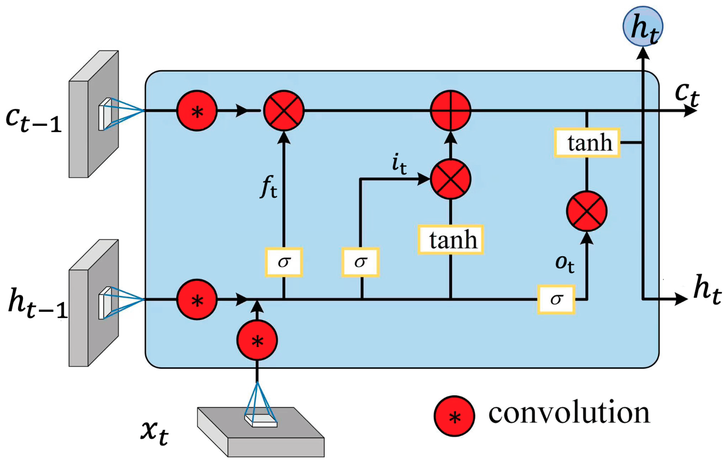
The ConvLSTM model adopts the sequence-to-sequence recurrent network architecture proposed by Sutskever et al. in 2014 [26], which was first extended to the field of spatiotemporal data prediction by Srivastava et al. in 2015 [27]. In our ConvLSTM network, all input states , memory states , hidden states , and various gating signals are manifested as three-dimensional tensors . Here, the first dimension represents the number of channels for the input data transformed into image data or the channels of hidden state features. The latter two dimensions represent the rows M and columns N of the hidden states in spatial scale, which can be envisioned as vectors of length P standing on a spatial grid with an area of M × N. The structure of the ConvLSTM unit is illustrated in Figure 3.
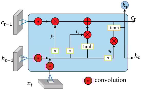
Figure 3.
The structure of the ConvLSTM unit.
Without considering the errors between the actual state and observed values, the specific computations for a ConvLSTM unit are as follows:
Here, represents the Hadamard operation (element-wise multiplication of matrices), and denotes the activation function. At time , represents the result of the computation after the information passes through the forget gate, represents the result after passing through the input gate, represents the cell state input at time t, represents the outcome after passing through the output gate, is the cell state at time t, and represents the output of the LSTM network at time t. In ConvLSTM, the connections between various gates and the input involve convolution operations, as do the interactions between states.
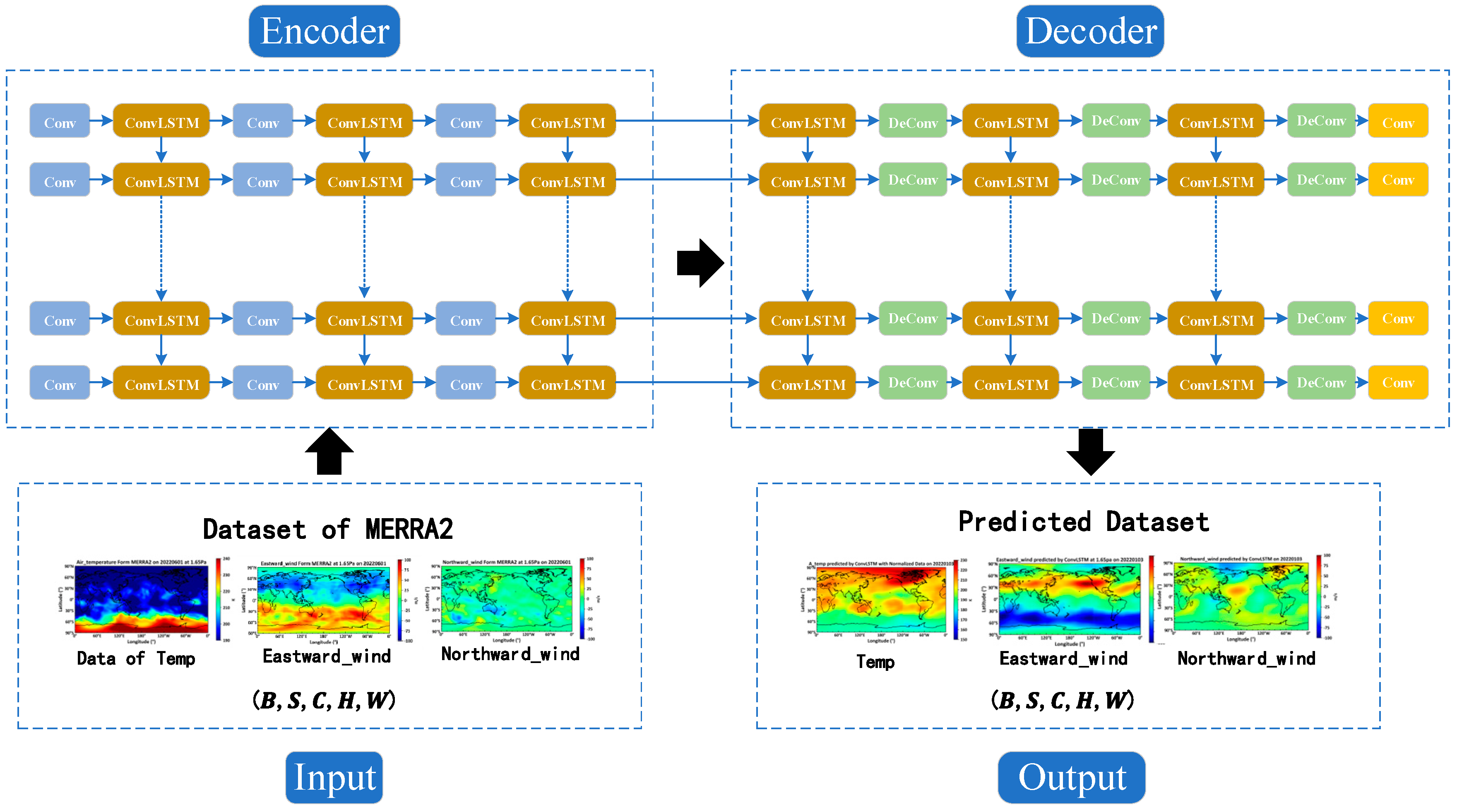
The workflow diagram for the near-space environment forecast model based on ConvLSTM is shown below in Figure 4.

Figure 4.
The workflow diagram of the ConvLSTM model.
The forecast model consists of four parts: the input layer, the encoder, the decoder, and the output layer. A detailed description of the structure of these four parts is provided below.
- The input layer: The matrix dimension of the input layer is denoted as (B, S, C, H, W), where B represents the batch size, indicating the number of samples processed concurrently in a single training iteration; S stands for sequence length, denoting the temporal length of a sample; C refers to the number of channels, indicating the number of channels in the data; H is the height, representing the vertical dimension of the data; and W is the width, denoting the horizontal extent of the data.
- The encoder is comprised of Convolutional Layers (Conv) and Convolutional LSTM (ConLSTM) units:
- (a)
- Conv is one of the commonly used layers in deep learning models, primarily utilized for extracting features from input data. Each convolutional layer is represented by an ordered dictionary, which contains the parameters required for the convolution operation. These parameters include: Input channel number, which specifies the number of channels in the input data; Output channel number, which determines the number of convolutional kernels and consequently the depth of the output feature map; Kernel size, which specifies the dimensions of the convolutional kernel; Stride, which determines the step length of the convolutional kernel as it slides over the input data, affecting the size of the output feature map; Padding, which involves adding zeros to the edges of the input data to control the size of the output feature map.
- (b)
- The ConLSTM unit, a specialized type of Recurrent Neural Network, integrates convolutional operations with the LSTM architecture. Each ConLSTM unit consists of a set of convolutional kernels and gating units (forget gate, input gate, and output gate), designed to capture spatio-temporal dependencies in sequential data. Within the encoder, the ConLSTM units receive feature representations from convolutional layers and utilize the convolutional kernels to slide along the sequence dimension, effectively capturing the spatio-temporal information of the input sequence.
- The decoder consists of Deconvolutional Layers (DeConv), Convolutional LSTM (ConLSTM), and Feature Mapping Recovery (Conv) processes: Deconvolutional layers are a primary component of the decoding layer, tasked with transforming the abstract representations from the encoded data back into the original data space.
- (a)
- The deconvolution process is the inverse of the convolution process, gradually restoring the resolution from a lower-resolution feature map to that of the original input. Each deconvolution layer contains a set of parameters, including the number of input channels, output channels, kernel size, stride, and padding.
- (b)
- Within the decoder, Convolutional LSTM units are also employed to handle spatio-temporal sequence data, progressively restoring the original data space.
- (c)
- The final phase of the decoding layer includes a feature mapping recovery step, which systematically transforms the abstract representations back to the form of the original data through convolution operations.
- The output layer: The matrix dimension of the output layer is identical to that of the input layer.
3.1.2. ConvGRU
The ConvGRU network represents a structural simplification over the ConvLSTM network. Ballas et al. [28] embedded the convolutional network into the Gated Recurrent Unit (GRU) [19] to achieve unified modeling of fine-grained spatiotemporal information. Besides retaining the capability to address long-term dependencies, the ConvGRU network features a simpler architecture, fewer parameters, and enhanced operational speed. The structure of the ConvGRU unit is illustrated in the Figure 5 below.
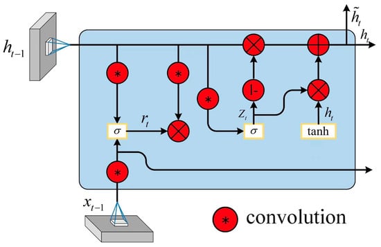
Figure 5.
The structure of the ConvGRU unit.
Unlike the three gate structures of the ConvLSTM network, the ConvGRU network comprises only two gates: the update gate and the reset gate. These mechanisms facilitate the memory and filtering of information. The update gate determines the degree to which information from the previous time step is retained, with values ranging from 0 to 1. A value closer to 0 indicates a greater disposition towards discarding information from the previous moment, causing the ConvGRU cell to diminish this information; conversely, a value closer to 1 suggests a tendency to preserve information from the previous time step. The function of the reset gate is to filter information from the previous time step. A reset gate value nearing 0 signifies that more of the previous moment’s information is discarded; on the other hand, a higher value indicates greater retention of information. Thus, the update gate enables the retention of more useful information during the model’s iterative computations, while the reset gate assists in blocking irrelevant information. Together, these gates collaborate to enhance the GRU network’s performance in sequential prediction tasks. The mathematical expression for the ConvGRU network is as follows:
In this context, represents the Hadamard operation (element-wise multiplication of matrices), and denotes the activation function. Here, is the reset gate, is the update gate, is the candidate output at time t, and is the actual output at time t.
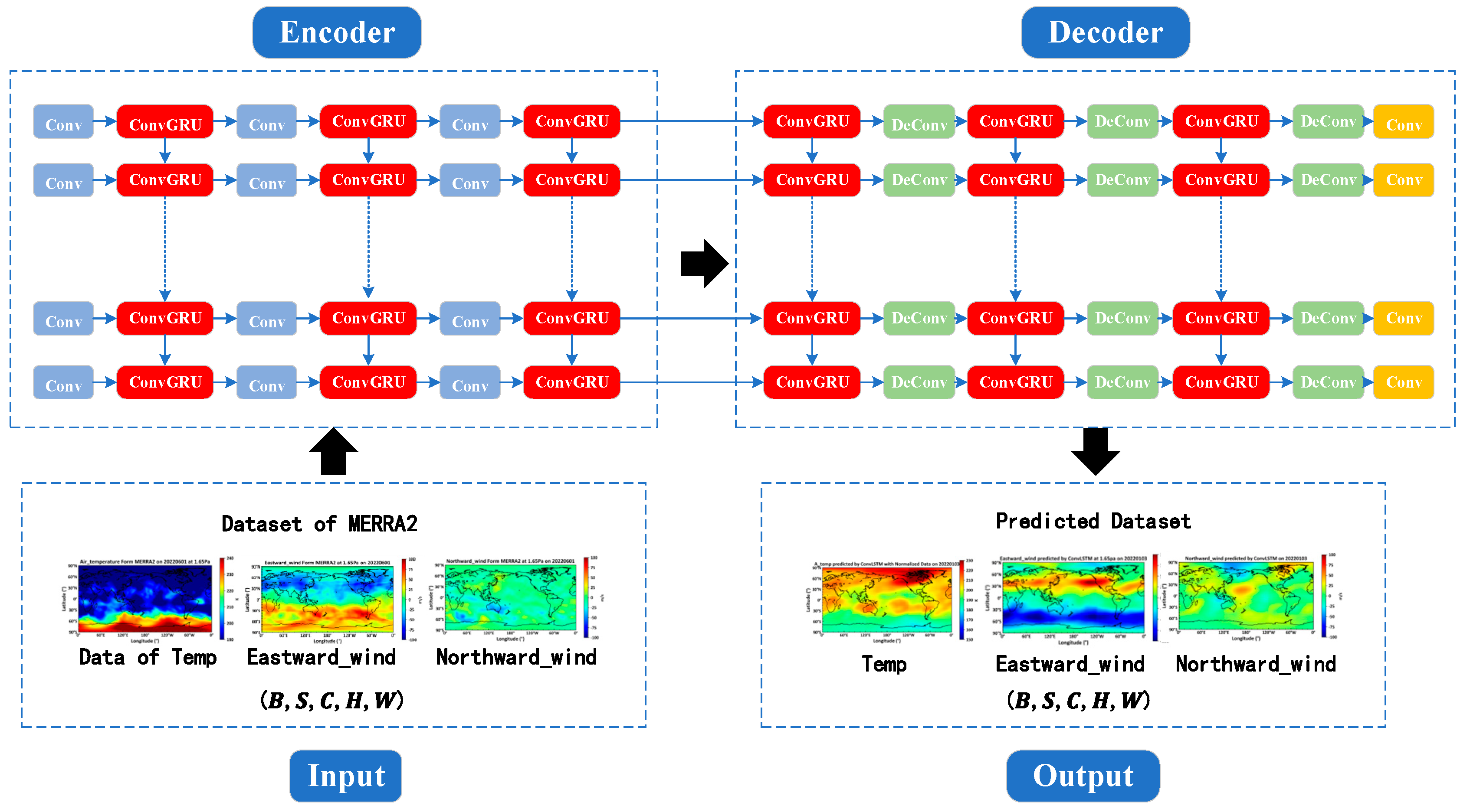
In our study, to investigate the differences in the capabilities of ConvLSTM and ConvGRU for processing spatiotemporal sequence data, the network structures and parameter settings of the proximate spatial environment forecasting models based on both are made identical. The network structure of the model based on ConvGRU also consists of four parts, with the only modification being the replacement of the ConvLSTM unit with a ConvGRU unit. The specific design is illustrated in Figure 6.
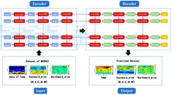
Figure 6.
The workflow diagram of the ConvGRU model.
3.2. Neural Network Parameter Configuration
This study demonstrates the feasibility of near-space atmospheric short-term forecasting on a global scale based on deep learning by training on MERRA2 data from 2011 to 2020, cross-validating with 2021 data, and testing with 2022 data, while comparing the merits of two algorithms through corresponding analyses.
The Table 1 below details the span and amount of data used in the training, validation, and test sets for forecasting the near-space atmosphere. The dataset spans 3653 days from 2011 to 2020 for training, 365 days in 2021 for validation, and 365 days in 2022 for testing, with a data ratio of approximately 10:1:1. The data include temperature, eastward wind, and northward wind at eight daily intervals.

Table 1.
Dataset details.
After preprocessing the data, it is necessary to configure the various parameters of the deep learning neural network constructed using ConvLSTM units. The parameters of the neural network built for this study are presented in the following Table 2.
Table 2.
The configuration of ConvLSTM.
As previously described, the parameter settings for the deep learning neural network built using ConvGRU units are as shown in the following Table 3.
Table 3.
The configuration of ConvGRU.
4. Discussion
This paper constructs neural networks with ConvLSTM and ConvGRU units to train on ten years of MERRA2 data for temperature, eastward wind, and northward wind, and to cross-validate with one year of data over 100 iterations. The following eight models were developed, allowing for short-term forecasts of temperature, eastward wind, and northward wind for eight time periods of the subsequent day, based on the previous day’s data from the MERRA2 dataset.
Spatially, the input consists of global-scale temperature, eastward wind, and northward wind data (for an example, see 2 June 2022) covering 72 isobaric surfaces, aiming to predict the corresponding values of temperature, eastward wind, and northward wind for the next day in the same spatial domain (for an example, see 3 June 2022). Temporally, the input includes data from eight-time intervals of the previous day (specifically at 00:00, 03:00, 06:00, 09:00, 12:00, 15:00, 18:00, and 21:00 on 2 June 2022), with the output providing forecasts for the same time intervals on the following day (at 00:00, 03:00, 06:00, 09:00, 12:00, 15:00, 18:00, and 21:00 on 3 June 2022). By analyzing the discrepancies between the forecasted environmental values and the actual measurements, the usability of the method and the strengths and weaknesses of the model are assessed.
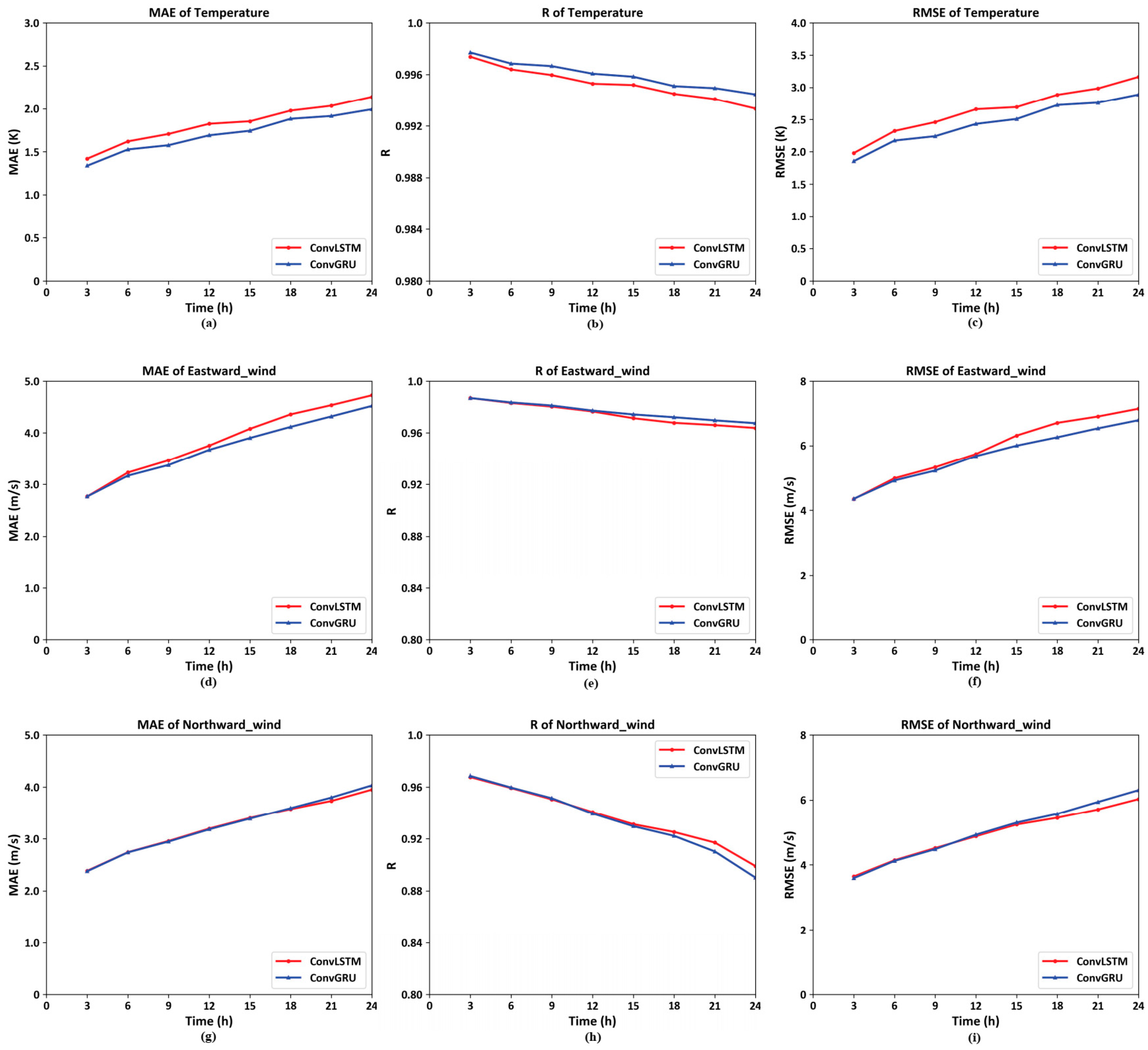
4.1. Predictive Accuracy
In terms of timing, the input data cover eight time segments per day, exemplified by the intervals at 03:00, 06:00, 09:00, 12:00, 15:00, 18:00, 21:00, and 24:00 on 2 January 2022. The output consists of predicted values for the corresponding eight-time segments on the following day, 3 January 2022, at the same time. By calculating the Mean Absolute Error (MAE), correlation coefficient (R), and Root Mean Square Error (RMSE) for these eight time points against actual data (from MERRA2), it was observed that both models demonstrated a trend of decreasing predictive accuracy with increasing time span. Moreover, the model trained using ConvGRU units performed better than that using ConvLSTM units. This finding aligns with the conclusions drawn by Shi et al. in their study, which indicated superior performance of ConvGRU [17].
The model trained to use the previous day’s temperature values predicts the root mean square error (RMSE) for temperature values at various altitudes in the first three hours of the next day to be approximately 1.8 K in Figure 7. The RMSE for the predicted eastward and northward wind values compared to the actual measurements also displays notable accuracy, with values of 4.2 m/s and 3.8 m/s in Figure 7, respectively. Moreover, as time progresses, the neural network built with ConvGRU units demonstrates superior performance over the one constructed with ConvLSTM units. Although the former has a simpler structure, it captures long-term temporal information more effectively. This not only supports the reliability of the developed model but also offers guidance for future long-term predictions of near-space atmospheric elements.
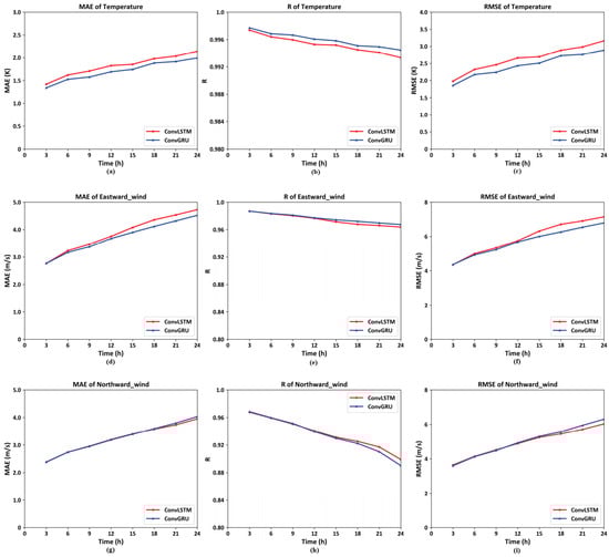
Figure 7.
The predictive accuracy of eight-time segments per day. ((a–c): The MAE, R and RMSE Curve of temperature on 72 isobaric surfaces on global scales at eight time periods on 3 January 2022. (d–f): The MAE, R and RMSE Curve of northward wind on 72 isobaric surfaces on global scales at eight time periods on 3 January 2022. (g–i): The MAE, R and RMSE Curve of eastward wind on 72 isobaric surfaces on global scales at eight time periods on 3 January 2022).
4.2. Models Comparison
To refine the study of the accuracy in short-term forecasting for temperature, eastward wind, and northward wind, as well as the differences between the two models, we employed the trained models to predict the near-space atmospheric factors on 3 June 2022.
4.2.1. Temperature
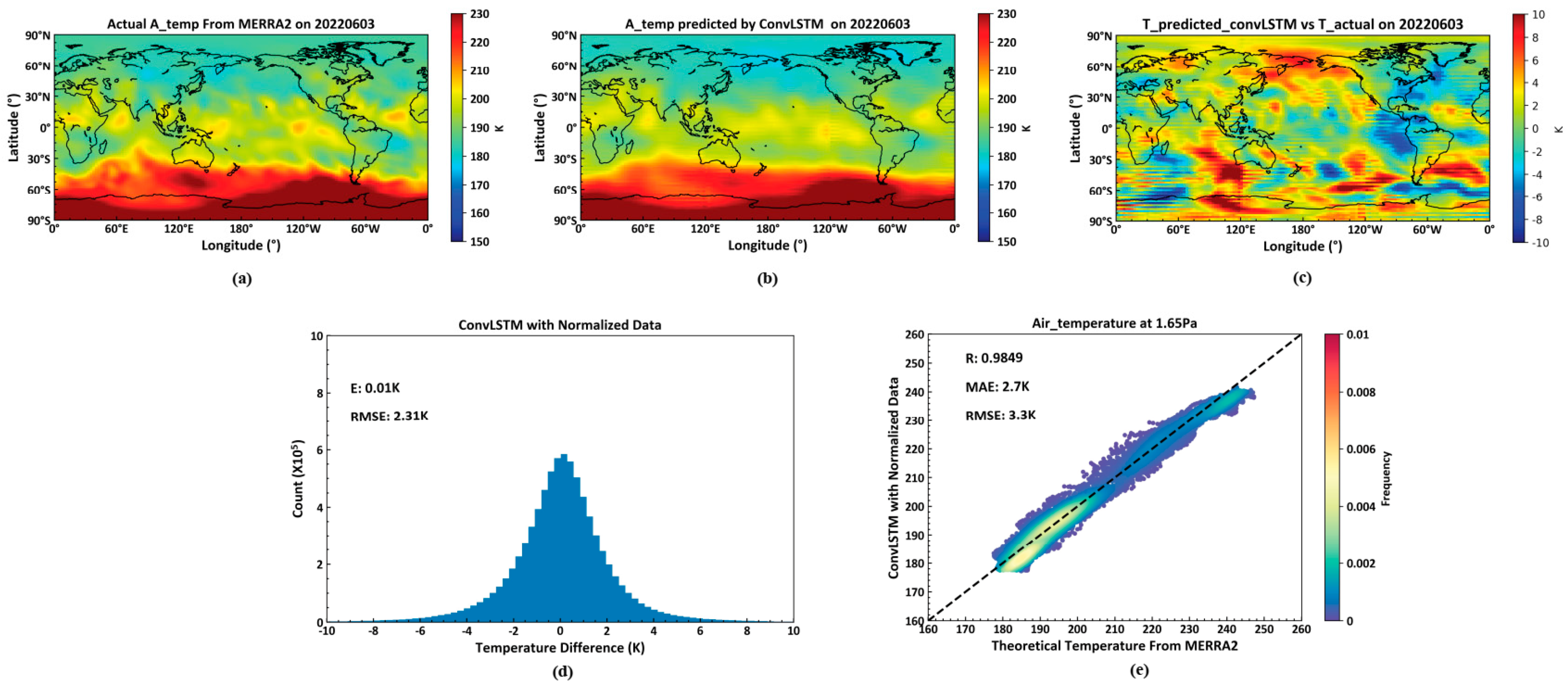
A random experiment on temperature forecasting was conducted on 3 June 2022, across 72 global isobaric surfaces, revealing a root mean square error of all temperature values at 2.31 K, indicating high precision [20] Temperature profiles demonstrate that short-term temperature forecasts not only predict major trends accurately but also yield good results for sudden temperature increases on a smaller scale. At a higher altitude (on the 1.65 Pa isobaric surface, approximately 70 km above sea level), the correlation coefficient between predicted and actual temperature values reaches 98.49%. This finding is significantly meaningful for short-term temperature forecasts in near space and for exploring the physical mechanisms related to temperature variations in this region.
As illustrated in Figure 8, (a) shows the actual temperature data on 3 June 2022, at the 1.65 Pa isobaric surface height from the MERRA2 dataset. (b) displays the temperature data for the same date and isobaric height, predicted by a model trained using a deep learning neural network based on the ConvLSTM unit, utilizing the MERRA2 data from 2 June 2022. (c) is the pseudocolor map of the difference between actual temperature and predicted temperature. (d) indicates the average and root mean square errors between the actual temperatures across all 72 isobaric surfaces globally on 3 June 2022, and those predicted by the ConvLSTM-based model. Lastly, (e) presents the correlation coefficient, average error, and root mean square error between the actual and predicted temperature values at the 1.65 Pa isobaric surface height.

Figure 8.
Predicted Temperature by ConvLSTM. (a): the actual temperature data on 3 June 2022; (b): the temperature predicted by GonvLSTM on 3 June 2022; (c): the differences between actual temperature data and predicted data on 3 June 2022; (d): the average and root mean square errors between the actual temperatures and predicted data on 3 June 2022; (e): the correlation coefficient, average error, and root mean square error between the actual data and predicted temperature data on 3 June 2022.
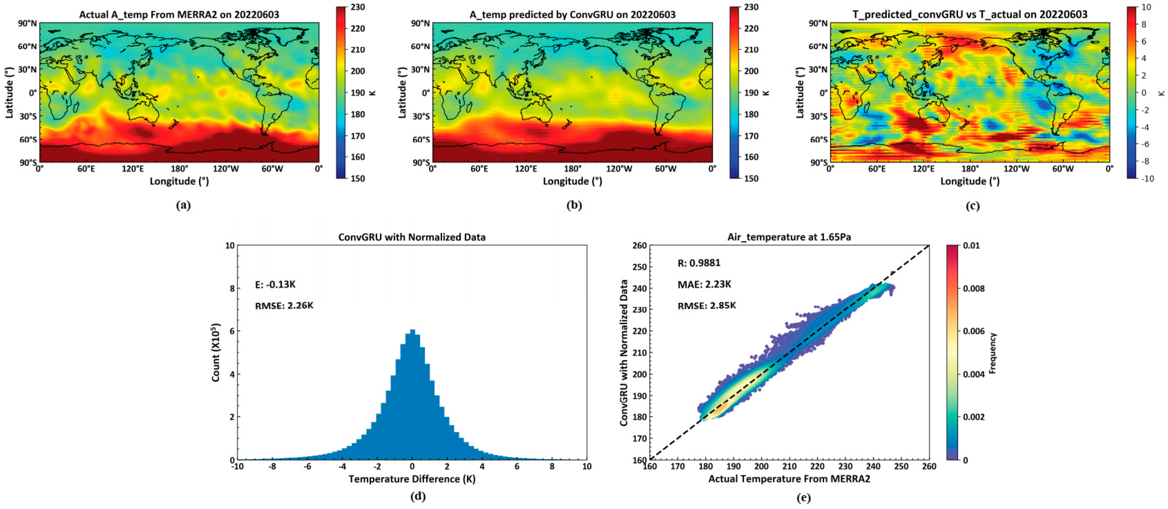
As illustrated in Figure 9, (a) shows the actual temperature data on 3 June 2022, at the 1.65 Pa isobaric surface height from the MERRA2 dataset. (b) displays the temperature data for the same date and isobaric height, predicted by a model trained using a deep learning neural network based on the ConvGRU unit, utilizing the MERRA2 data from 2 June 2022. (c) is the pseudocolor map of the difference between actual temperature and predicted temperature. (d) indicates the average and root mean square errors between the actual temperatures across all 72 isobaric surfaces globally on 3 June 2022, and those predicted by the ConvGRU-based model. Lastly, (e) presents the correlation coefficient, average error, and root mean square error between the actual and predicted temperature values at the 1.65 Pa isobaric surface height.

Figure 9.
Predicted Temperature by ConvGRU. (a): the actual temperature data on 3 June 2022; (b): the temperature predicted by GonvGRU on 3 June 2022; (c): the differences between actual temperature data and predicted data on 3 June 2022; (d): the average and root mean square errors between the actual temperatures and predicted data on 3 June 2022; (e): the correlation coefficient, average error, and root mean square error between the actual data and predicted temperature data on 3 June 2022.
A deep learning network model constructed using ConGRU units across 72 isobaric surfaces on a global scale predicted temperature data with a root mean square error (RMSE) of 2.26 K. This performance surpasses that of models built with ConvLSTM units. However, at the 1.65 Pa isobaric surface, the RMSE of the predicted temperature relative to the actual temperature was 2.85 K, which represents a 13.6% improvement over the 3.3 K RMSE observed in models constructed with ConvLSTM units.
4.2.2. Eastward Wind
The model trained using a neural network built with ConvLSTM units demonstrates favorable outcomes in predicting the eastward wind over 72 isobaric surfaces on a global scale, with a root mean square error (RMSE) of 5.03 m/s for near-space zonal wind forecasts over a 24-h period. Moreover, at the 1.65 Pa isobaric surface (approximately 70 km altitude), the RMSE for eastward wind is 6.07 m/s, which shows an improvement over ground-based meteor radar observations (which measure wind fields between altitudes of 70 km and 110 km) as documented in the literature. Additionally, upon evaluating actual numerical values of eastward winds across multiple isobaric surfaces, it was observed that near the equator, the values of eastward winds are typically around 0 m/s. This results in a degradation of performance metrics such as correlation coefficient, mean error, and RMSE for eastward wind forecasts in equatorial regions.
As illustrated in Figure 10, (a) displays actual eastward wind data from the MERRA2 dataset on 3 June 2022, at the 1.65 Pa isobaric level. (b) shows temperature data predicted by a deep learning neural network, constructed using ConvLSTM as the basic unit, based on MERRA2 dataset data from 2 June 2022. (c) is the pseudocolor map of the difference between actual temperature and predicted temperature. (d) presents the global scale average error and root mean square error (RMSE) between actual eastward winds and predicted temperatures by the ConvLSTM model across all 72 isobaric levels for 3 June 2022. (e) shows the correlation coefficient, average error, and RMSE between actual and predicted eastward wind values at the 1.65 Pa level.
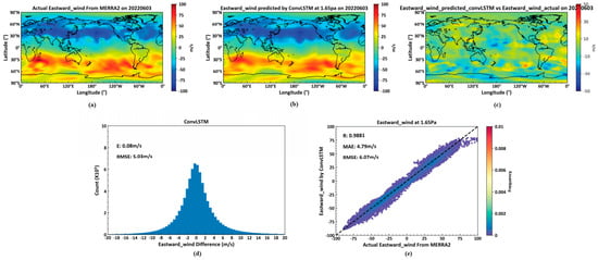
Figure 10.
Predicted Eastward Wind by ConvLSTM. (a): the actual Eastward Wind data on 3 June 2022; (b): the Eastward Wind predicted by GonvLSTM on 3 June 2022; (c): the differences between actual Eastward Wind data and predicted data on 3 June 2022; (d): the average and root mean square errors between the actual Eastward Wind and predicted data on 3 June 2022; (e): the correlation coefficient, average error, and root mean square error between the actual data and predicted Eastward Wind data on 3 June 2022.
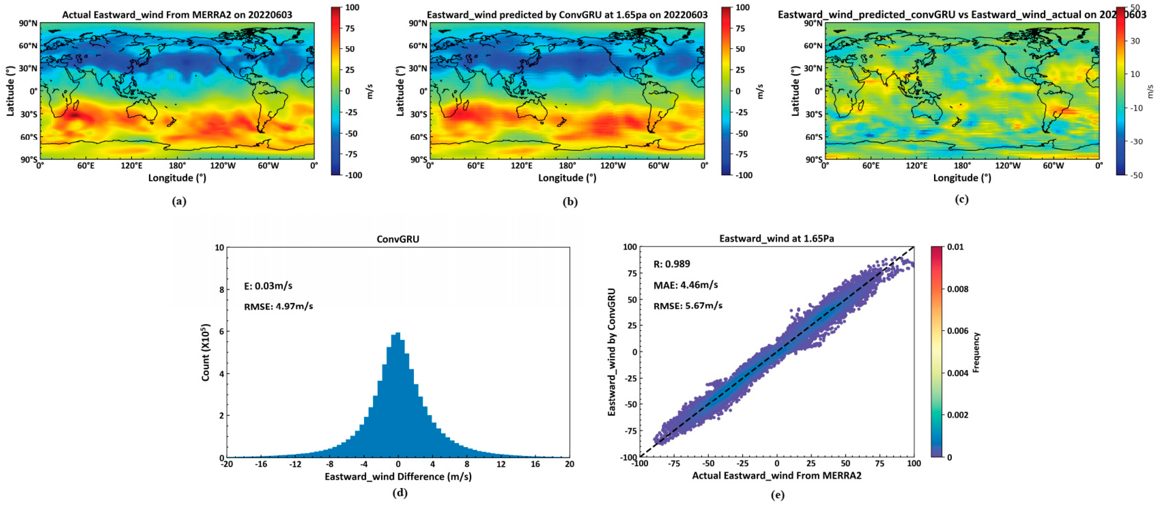
Figure 11 depicts, (a), actual eastward wind data from the MERRA2 dataset on 3 June 2022, at the 1.65 Pa isobaric height. (b) features data predicted by a deep learning neural network built with ConvGRU as the foundational element, using data from 2 June 2022, from the MERRA2 dataset. (c) is the pseudocolor map of the difference between actual temperature and predicted temperature. (d) details the average error and RMSE for actual versus predicted eastward winds across all 72 isobaric levels globally on 3 June 2022, by the ConvGRU model. (e) provides the correlation coefficient, average error, and RMSE for actual and predicted eastward winds at the 1.65 Pa level.
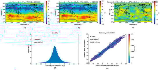
Figure 11.
Predicted Eastward by ConvGRU. (a): the actual Eastward Wind data on 3 June 2022; (b): the Eastward Wind predicted by GonvGRU on 3 June 2022; (c): the differences between actual Eastward Wind data and predicted data on 3 June 2022; (d): the average and root mean square errors between the actual Eastward Wind and predicted data on 3 June 2022; (e): the correlation coefficient, average error, and root mean square error between the actual data and predicted Eastward Wind data on 3 June 2022.
A neural network constructed using ConvGRU units and trained on data predicts eastward winds across 72 global isobaric levels more effectively than those constructed with ConvLSTM units. For global-scale predictions within a single day across 72 levels, the predicted RMSE is 4.97 m/s, while at the 1.65 Pa level, it achieves an RMSE of 5.67 m/s, representing a 6.6% improvement over the ConvLSTM model.
4.2.3. Northward Wind
The model trained using ConvLSTM neural network cells demonstrates commendable performance in predicting northward winds at 72 isobaric surfaces globally, with a root mean square error (RMSE) of 4.25 m/s for near-space zonal winds prediction over one day. The zonal wind RMSE at the 1.65 Pa isobaric level (approximately 70 km altitude) is 5.35 m/s, which is superior to ground-based meteor radar observations (70 km–110 km altitude) of northward winds, as cited in the literature.
As shown in Figure 12, (a) displays actual northward wind data on 3 June 2022, at the 1.65 Pa isobaric height from the MERRA2 dataset. (b) presents northward wind predictions at the same height for 3 June 2022, based on the previous day’s MERRA2 data, generated by a deep learning neural network constructed with ConvLSTM cells. (c) is the pseudocolor map of the difference between actual temperature and predicted temperature. (d) illustrates the average and root mean square errors between actual and predicted northward winds across all 72 isobaric surfaces globally on 3 June 2022. (e) details the correlation coefficient, mean error, and RMSE for northward winds at the 1.65 Pa height.
Figure 12.
Predicted Northward Wind by ConvLSTM. (a): the actual Northward Wind data on 3 June 2022; (b): the Northward Wind predicted by GonvLSTM on 3 June 2022; (c): the differences between actual Northward Wind data and predicted data on 3 June 2022; (d): the average and root mean square errors between the actual Northward Wind and predicted data on 3 June 2022; (e): the correlation coefficient, average error, and root mean square error between the actual data and predicted Northward Wind data on 3 June 2022.
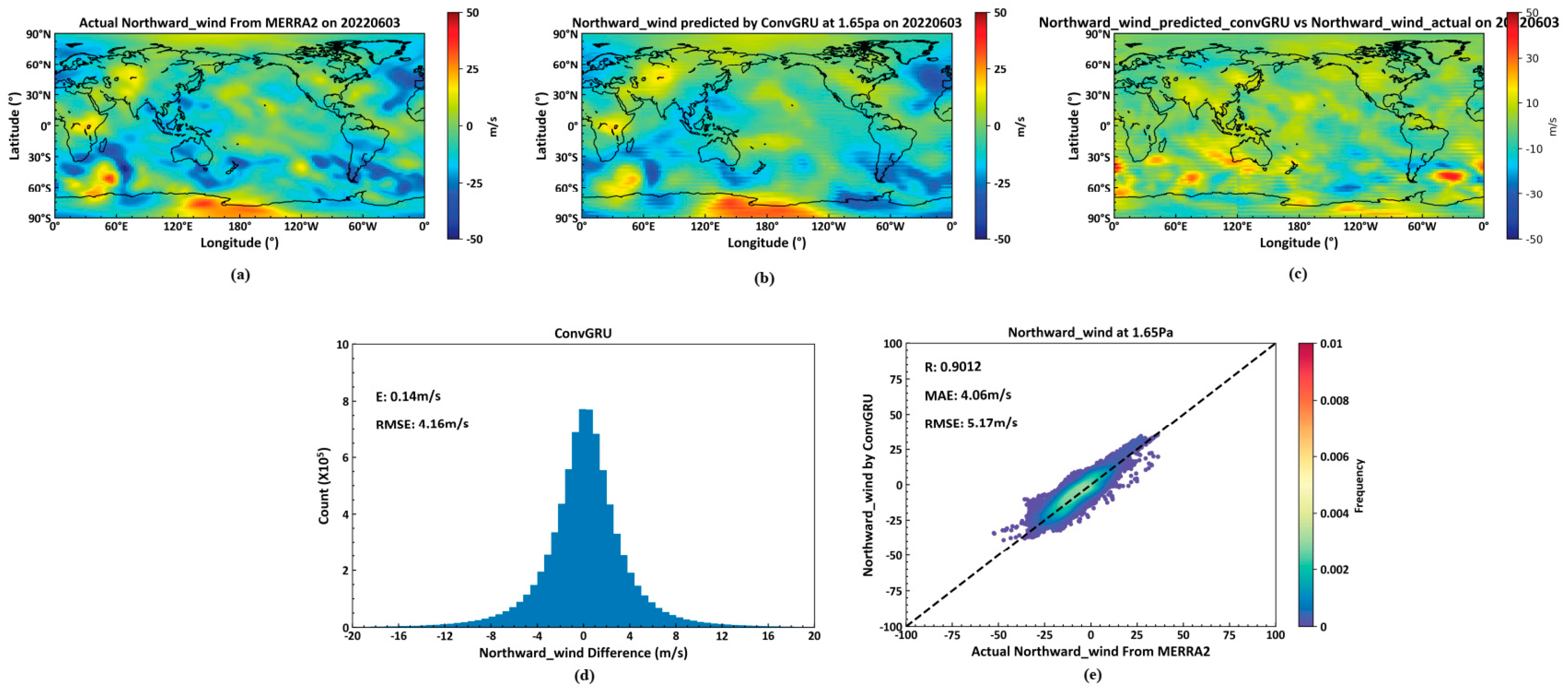
Figure 13 depicts, (a), actual northward wind data from the MERRA2 dataset on 3 June 2022, at the 1.65 Pa isobaric height. (b) shows northward wind predictions for the same day and height, generated by a deep learning neural network constructed with ConvGRU cells, based on data from 2 June 2022. (c) is the pseudocolor map of the difference between actual temperature and predicted temperature. (d) displays average and RMSE errors for the actual versus predicted northward winds at all 72 global isobaric surfaces on 3 June 2022. (e) shows the correlation coefficient, average error, and RMSE for northward winds at the 1.65 Pa height.
Figure 13.
Predicted Northward wind by ConvGRU. (a): the actual Northward Wind data on 3 June 2022; (b): the Northward Wind predicted by GonvGRU on 3 June 2022; (c): the differences between actual Northward Wind data and predicted data on 3 June 2022; (d): the average and root mean square errors between the actual Northward Wind and predicted data on 3 June 2022; (e): the correlation coefficient, average error, and root mean square error between the actual data and predicted Northward Wind data on 3 June 2022.
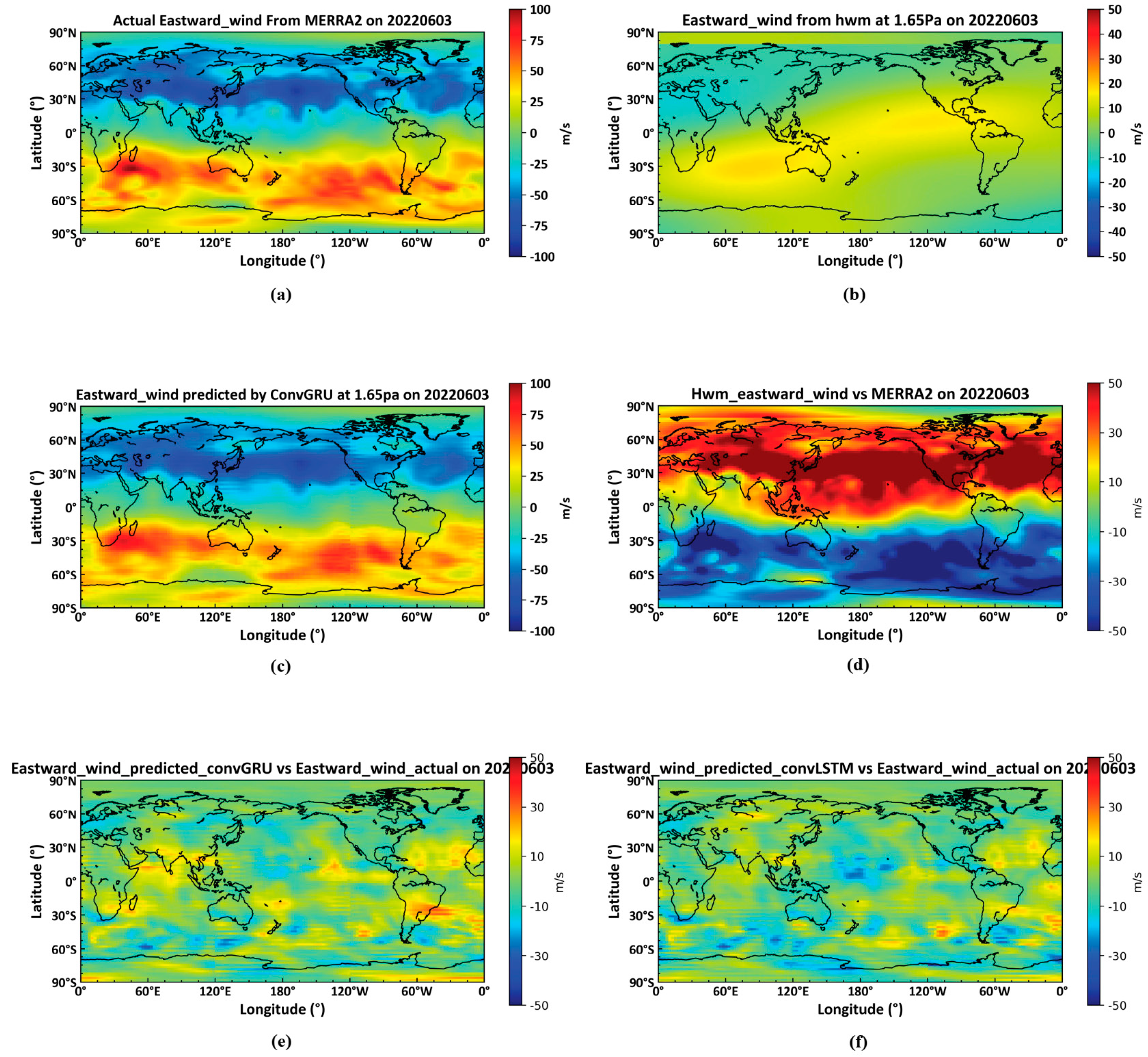
Tao Liu [10] used the time series model to predict the wind field at 88 km in the area of Langfang, China, the standard deviation of the model prediction was 12.8 m/s. In contrast, our forecasting accuracy in predicting northward winds across 72 global isobaric surfaces, with a global RMSE of 4.16 m/s and 5.17 m/s at the 1.65 Pa height in Figure 13. We also use the numerical model HWM to predict the near-space wind field at the global scale of 1.65 Pa on 3 June 2022 in Figure 14. The standard deviation between the zonal wind and the true value in the actual MERRA2 dataset is 36.46 m/s, and the standard deviation of the meridional wind is 46.04 m/s.
Figure 14.
Model performance vs. HWM model. (a): the actual Eastward Wind data on 3 June 2022; (b): the predicted Eastward Wind data by HWM model; (c): the predicted Eastward Wind data by ConvGRU model; (d): the differences between actual Eastward Wind data and data predicted by HWM model; (e): the differences between actual Eastward Wind data and data predicted by ConvGRU model; (f): the differences between actual Eastward Wind data and data predicted by ConvLSTM model.
In summary, both neural networks constructed with ConvGRU and ConvLSTM cells exhibit strong performance in short-term forecasts of environmental elements such as near-space temperature, zonal winds, and northward winds. Both are capable of effectively predicting the next day’s environmental conditions; however, the ConvGRU approach proves to be more effective than the ConvLSTM model.
4.2.4. Performance at Different Isobaric Surfaces
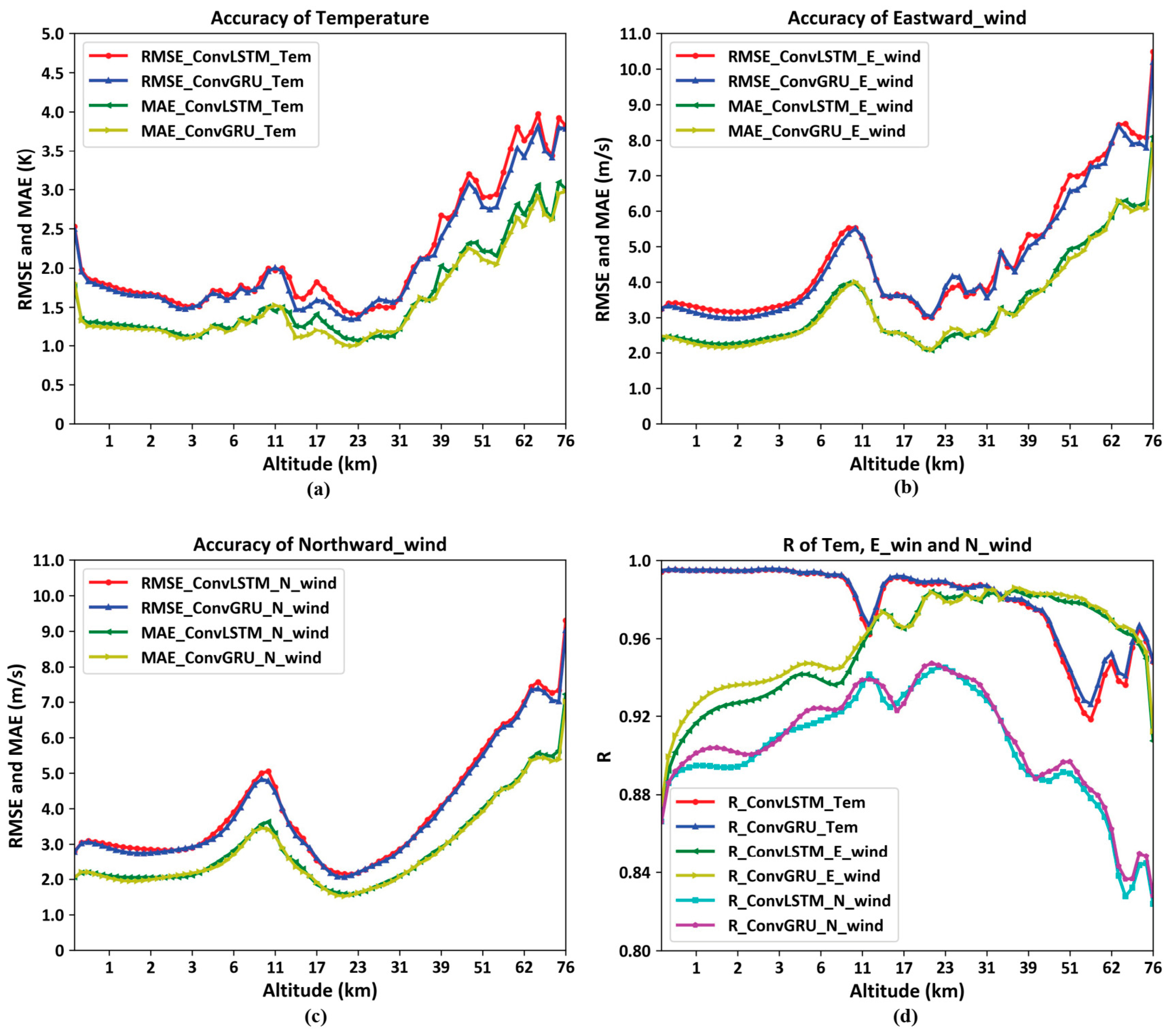
By statistically analyzing the correlation coefficients, mean errors, and root mean square errors between the predicted and actual values at different 72 isobaric surfaces for the entire year of 2022 and at various latitudes and longitudes, the following figure is obtained.
As illustrated in Figure 15d shows the correlation coefficient curves of temperature, eastward wind, and northward wind at 72 isobaric surfaces, the others depict the mean error curves and the root mean square error curves of temperature, eastward wind, and northward wind at 72 isobaric surfaces. The following conclusions can be drawn: The models trained through deep learning using ConvGRU and ConvLSTM effectively predict environmental variables at various altitudes, though the prediction accuracy generally decreases to varying degrees as the altitude increases, which is related to the higher reliability of the MERRA2 dataset at lower altitudes. Furthermore, at altitudes around 10 km and 52 km, corresponding to the interface between the troposphere and stratosphere, and the interface between the stratosphere and mesosphere, respectively, complex atmospheric changes, dynamical-thermodynamic features, and intrinsic mechanisms exist, leading to varying degrees of degradation in the prediction accuracy of temperature, eastward wind, and northward wind.
Figure 15.
Model performance at different 72 isobaric surfaces. (a): the accuracy of temperature; (b): the accuracy of Eastward Wind; (c) the accuracy of Northward Wind; (d): the correlation coefficient of temperature, Eastward Wind and Northward Wind.
4.2.5. Performance at Different Latitudes
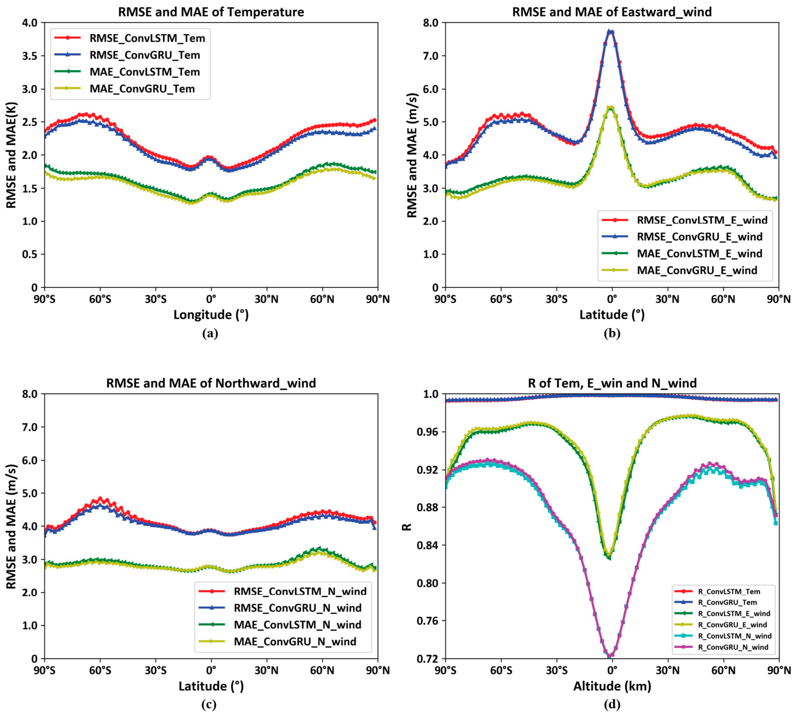
By statistically analyzing the correlation coefficients, mean errors, and root mean square errors between the predicted and actual values at different 96 latitudes for the entire year of 2022 and at various altitudes and longitudes, the following curve plots are obtained.
As depicted in Figure 16d shows the correlation coefficient curves of temperature, eastward wind, and northward wind at 96 latitudes, the others display the mean error curves and the root mean square error curves of temperature, eastward wind, and northward wind at 96 latitudes. The following conclusions can be drawn: The models trained through deep learning using ConvGRU and ConvLSTM effectively predict environmental variables at various latitudes, with ConvGRU performing slightly better. Near the polar regions, the prediction results of both models do not exhibit a significant decline, as the MERRA2 dataset utilizes the real-time atmospheric temperature values obtained from the Microwave Limb Sensor (MLS) on the MODIS Aura satellite, which provides improved calibration coefficients for better atmospheric correction in polar regions [29,30]. This corroborates the conclusion that the MERRA2 dataset has relatively high reliability in polar regions. However, when predicting eastward wind, a considerable decrease in the correlation coefficient is observed near the equatorial regions, accompanied by an increase in mean error and root mean square error, which is related to the fact that the eastward wind values are essentially zero near the equator, as mentioned earlier.
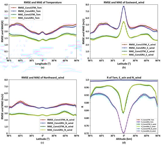
Figure 16.
Model performance at different 96 latitudes surfaces. (a): the accuracy of temperature; (b): the accuracy of Eastward Wind; (c) the accuracy of Northward Wind; (d): the correlation coefficient of temperature, Eastward Wind and Northward Wind.
5. Conclusions
In this study, we constructed neural networks based on ConvLSTM and ConvGRU units to perform deep learning on a ten-year dataset from MERRA2, obtaining a global-scale short-term forecasting model (daily forecast) for the near-space atmosphere. The model’s effectiveness was validated through testing on the 2022 dataset, demonstrating that deep learning is a promising approach for near-space atmospheric forecasting. Additionally, through model comparison and spatiotemporal analysis, the following conclusions were drawn:
- When predicting eight different times in a day, as the time span increases, the model’s prediction accuracy tends to decrease, and the ConvGRU model outperforms the ConvLSTM model in forecasting results.
- In a comparison experiment using randomly selected data from 2 June 2022, to predict the environmental parameters for 3 June 2022, the ConvGRU model performed better than the ConvLSTM model in forecasting temperature, eastward wind, and northward wind, with smaller root-mean-square errors (RMSEs). Specifically, at the 1.65 Pa pressure level, the ConvGRU model showed a significant improvement in prediction accuracy over the ConvLSTM model, with a 13.6% improvement in temperature, a 6.6% improvement in the eastward wind, and an 8.8% improvement in the northward wind.
- By evaluating the correlation coefficients, mean errors, and root-mean-square errors between the predicted and actual values across different pressure levels (72 levels in total) for the entire year of 2022 and various latitudes and longitudes, it was found that the models’ forecasting capability decreases with increasing altitude. Furthermore, both models exhibited significant decreases in forecasting accuracy for temperature, eastward wind, and northward wind at the interfaces between the Troposphere and Stratosphere, and between the Stratosphere and Mesosphere, which is related to the complex atmospheric changes at these interfaces.
- By evaluating the correlation coefficients, mean errors, and root-mean-square errors between the predicted and actual values across different latitudes (96 latitudes in total) for the entire year of 2022 and various altitudes and longitudes, it was found that the model’s prediction accuracy in the polar regions was not significantly lower than other latitudes, indicating that the MERRA2 dataset has relatively high reliability in the polar regions.
The reliability of the MERRA2 dataset is not sufficiently high at higher altitudes, and environmental data for the near-space region above 70 km is missing. Therefore, it is worth considering using the output results of the trained model as the initial field for the WACCM numerical model and utilizing the WACCM numerical model to forecast environmental parameters above 70 km in altitude. Chen B. [17] designed a neural operator method to predict regional wind fields in the middle and upper atmosphere. The accuracy of regional wind behaves better than ConvLSTM. Chen B.’s research points out the next direction of work for this article to improve the method used in this article. K.A. Alex [22] improves the accuracy of predicting wind power by filtering out the noise effectively. In the next work, we will try to discuss the noise of temperature and wind field data in the MERRA-2 dataset. We will use certain data processing methods to remove some kinds of noise in the data so that we can improve the prediction accuracy of temperature and wind fields.
Author Contributions
Conceptualization, X.S., C.Z., J.F. and Y.L.; methodology, X.S., Y.Z. and C.Z.; investigation, J.F., T.X., Z.D. and Z.C.; validation, Z.C.; formal analysis, X.S. and Y.L.; resources, T.L. and Z.Z.; visualization, H.Y. and T.L.; funding acquisition, Y.L. and T.X. All authors have read and agreed to the published version of the manuscript.
Funding
This research was funded by the National Natural Science Foundation of China (NSFC grant No. 42204161), the Hubei Natural Science Foundation (grant No. 2023AFB200, 2022CFB651).
Institutional Review Board Statement
Not applicable.
Informed Consent Statement
Not applicable.
Data Availability Statement
The use of MERRA-2 data was provided by NASA (NASA’s latest generation of high spatial and temporal resolution global atmospheric reanalysis data, https://rda.ucar.edu/datasets/ds313.3/dataaccess/#, accessed on 20 December 2023).
Conflicts of Interest
The authors declare that they have no conflict of interest.
References
- Chen, H. An overview of the space-based observations for upper atmospheric research. Adv. Earth Sci. 2009, 24, 229. [Google Scholar]
- Tomme, E.B.; Phil, D. The Paradigm Shift to Effects-Based Space: Near-Space as a Combat Space Effects Enabler; Airpower Research Institute, College of Aerospace Doctrine, Research and Education, Air University: Islamabad, Pakistan, 2005. [Google Scholar]
- Goncharenko, L.P.; Chau, J.L.; Liu, H.L.; Coster, A.J. Unexpected connections between the stratosphere and ionosphere. Geophys. Res. Lett. 2010, 37. [Google Scholar] [CrossRef]
- Drob, D.P.; Emmert, J.T.; Meriwether, J.W.; Makela, J.J.; Doornbos, E.; Conde, M.; Hernandez, G.; Noto, J.; Zawdie, K.A.; McDonald, S.E.; et al. An update to the Horizontal Wind Model (HWM): The quiet time thermosphere. Earth Space Sci. 2015, 2, 301–319. [Google Scholar] [CrossRef]
- Picone, J.M.; Hedin, A.E.; Drob, D.P.; Aikin, A.C. NRLMSISE-00 empirical model of the atmosphere: Statistical comparisons and scientific issues. J. Geophys. Res. Space Phys. 2002, 107, SIA 15-1–SIA 15-16. [Google Scholar] [CrossRef]
- Liu, H.L.; Bardeen, C.G.; Foster, B.T.; Lauritzen, P.; Liu, J.; Lu, G.; Marsh, D.R.; Maute, A.; McInerney, J.M.; Pedatella, N.M.; et al. Development and validation of the whole atmosphere community climate model with thermosphere and ionosphere extension (WACCM-X 2.0). J. Adv. Model. Earth Syst. 2018, 10, 381–402. [Google Scholar] [CrossRef]
- Allen, D.R.; Eckermann, S.D.; Coy, L.; McCormack, J.P.; Hogan, T.F.; Kim, Y.J. P2. 4 Stratospheric Forecasting with Nogaps-Alpha. Available online: https://www.researchgate.net/profile/Young-Joon-Kim-7/publication/235120361_Stratospheric_Forecasting_with_NOGAPS-ALPHA/links/00b49530e63dd0e3b3000000/Stratospheric-Forecasting-with-NOGAPS-ALPHA.pdf (accessed on 11 August 2024).
- Greenberg, D.A.; Dupont, F.; Lyard, F.H.; Lynch, D.R.; Werner, F.E. Resolution issues in numerical models of oceanic and coastal circulation. Cont. Shelf Res. 2007, 27, 1317–1343. [Google Scholar] [CrossRef]
- Roney, J.A. Statistical wind analysis for near-space applications. J. Atmos. Sol.-Terr. Phys. 2007, 69, 1485–1501. [Google Scholar] [CrossRef]
- Liu, T. Research on Statistical Forecasting Method of Atmospheric Wind Field in Adjacent Space; National Space Science Center of Chinese Academy of Sciences: Beijing, China, 2017. [Google Scholar]
- Chen, B.; Sheng, Z.; He, Y. High-Precision and Fast Prediction of Regional Wind Fields in Near Space Using Neural-Network Approximation of Operators. Geophys. Res. Lett. 2023, 50, e2023GL106115. [Google Scholar] [CrossRef]
- Bi, K.; Xie, L.; Zhang, H.; Chen, X.; Gu, X.; Tian, Q. Accurate medium-range global weather forecasting with 3D neural networks. Nature 2023, 619, 533–538. [Google Scholar] [CrossRef]
- Kaparakis, C.; Mehrkanoon, S. Wf-unet: Weather fusion unet for precipitation nowcasting. arXiv 2023, arXiv:2302.04102. [Google Scholar]
- Nguyen, T.; Brandstetter, J.; Kapoor, A.; Gupta, J.K.; Grover, A. Climax: A foundation model for weather and climate. arXiv 2023, arXiv:2301.10343. [Google Scholar]
- Lam, R.; Sanchez-Gonzalez, A.; Willson, M.; Wirnsberger, P.; Fortunato, M.; Alet, F.; Ravuri, S.; Ewalds, T.; Eaton-Rosen, Z.; Hu, W.; et al. GraphCast: Learning skillful medium-range global weather forecasting. arXiv 2022, arXiv:2212.12794. [Google Scholar]
- Bi, K.; Xie, L.; Zhang, H.; Chen, X.; Gu, X.; Tian, Q. Pangu-weather: A 3d high-resolution model for fast and accurate global weather forecast. arXiv 2022, arXiv:2211.02556. [Google Scholar]
- Chen, B.; Sheng, Z.; Cui, F. Refined short-term forecasting atmospheric temperature profiles in the stratosphere based on operators learning of neural networks. Earth Space Sci. 2024, 11, e2024EA003509. [Google Scholar] [CrossRef]
- Shi, X.; Chen, Z.; Wang, H.; Yeung, D.Y.; Wong, W.K.; Woo, W.C. Convolutional LSTM network: A machine learning approach for precipitation nowcasting. Adv. Neural Inf. Process. Syst. 2015, 28; Part of Advances in Neural Information Processing Systems 28 (NIPS 2015).
- Cho, K. Learning phrase representations using RNN encoder-decoder for statistical machine translation. arXiv 2014, arXiv:1406.1078. [Google Scholar]
- Bosilovich, M.G.; Robertson, F.R.; Takacs, L.; Molod, A.; Mocko, D. Atmospheric water balance and variability in the MERRA-2 reanalysis. J. Clim. 2017, 30, 1177–1196. [Google Scholar] [CrossRef]
- Koster, R.D.; McCarty, W.; Coy, L.; Gelaro, R.; Huang, A.; Merkova, D.; Smith, E.B.; Sienkiewicz, M.; Wargan, K. MERRA-2 Input Observations: Summary and Assessment; NASA: Washington, DC, USA, 2016.
- Luke, K.A.A.; David, P.E.; Anandhakumar, P. Short-term wind power prediction using deep learning approaches. Adv. Comput. 2024, 132, 111–139. [Google Scholar]
- Duo, C.; Yong, Y.; Jiancan, L.; Ciren, B. Applicability analysis of MERRA surface air temperature over the Qinghai-Xizang Plateau. Plateau Meteorol. 2016, 35, 337–350. [Google Scholar]
- Cheridito, P.; Jentzen, A.; Rossmannek, F. Non-convergence of stochastic gradient descent in the training of deep neural networks. J. Complex. 2021, 64, 101540. [Google Scholar] [CrossRef]
- Kim, S.; Hong, S.; Joh, M.; Song, S.K. Deeprain: Convlstm network for precipitation prediction using multichannel radar data. arXiv 2017, arXiv:1711.02316. [Google Scholar]
- Sutskever, I.; Vinyals, O.; Le, Q.V. Sequence to sequence learning with neural networks. Adv. Neural Inf. Process. Syst. 2014, 27, 3104–3112. [Google Scholar]
- Srivastava, N.; Mansimov, E.; Salakhudinov, R. Unsupervised learning of video representations using lstms. In Proceedings of the International Conference on Machine Learning, PMLR, Lille, France, 7–9 July 2015; pp. 843–852. [Google Scholar]
- Ballas, N.; Yao, L.; Pal, C.; Courville, A. Delving deeper into convolutional networks for learning video representations. arXiv 2015, arXiv:1511.06432. [Google Scholar]
- Palmer, T.N.; Shutts, G.J.; Hagedorn, R.; Doblas-Reyes, F.J.; Jung, T.; Leutbecher, M. Representing model uncertainty in weather and climate prediction. Annu. Rev. Earth Planet. Sci. 2005, 33, 163–193. [Google Scholar] [CrossRef]
- Gelaro, R.; McCarty, W.; Suárez, M.J.; Todling, R.; Molod, A.; Takacs, L.; Randles, C.A.; Darmenov, A.; Bosilovich, M.G.; Reichle, R.; et al. The modern-era retrospective analysis for research and applications, version 2 (MERRA-2). J. Clim. 2017, 30, 5419–5454. [Google Scholar] [CrossRef] [PubMed]


Disclaimer/Publisher’s Note: The statements, opinions and data contained in all publications are solely those of the individual author(s) and contributor(s) and not of MDPI and/or the editor(s). MDPI and/or the editor(s) disclaim responsibility for any injury to people or property resulting from any ideas, methods, instructions or products referred to in the content. |
© 2024 by the authors. Licensee MDPI, Basel, Switzerland. This article is an open access article distributed under the terms and conditions of the Creative Commons Attribution (CC BY) license (https://creativecommons.org/licenses/by/4.0/).