Article

Let It Snow: Intercomparison of Various Total and Snow Precipitation Data over the Tibetan Plateau

Laboratory for Climatology and Remote Sensing, Department of Geography, Philipps-University Marburg, 35032 Marburg, Germany
*
Author to whom correspondence should be addressed.
Atmosphere 2024, 15(9), 1076; https://doi.org/10.3390/atmos15091076
Submission received: 6 August 2024 / Revised: 28 August 2024 / Accepted: 2 September 2024 / Published: 5 September 2024
(This article belongs to the Section Meteorology)

Abstract

:
The Global Precipitation Measurement Mission (GPM) improved spaceborne precipitation data. The GPM dual-frequency precipitation radar (DPR) provides information on total precipitation (TP), snowfall precipitation (SF) and snowfall flags (surface snowfall flag (SSF) and phase near surface (PNS)), among other variables. Especially snowfall data were hardly validated. This study compares GPM DPR TP, SF and snowfall flags on the Tibetan Plateau (TiP) against TP and SF from six well-known model-based data sets used as ground truth: ERA 5, ERA 5 land, ERA Interim, MERRA 2, JRA 55 and HAR V2. The reanalysis data were checked for consistency. The results show overall high agreement in the cross-correlation with each other. The reanalysis data were compared to the GPM DPR snowfall flags, TP and SF. The intercomparison performs poorly for the GPM DPR snowfall flags (HSS = 0.06 for TP, HSS = 0.23 for SF), TP (HSS = 0.13) and SF (HSS = 0.31). Some studies proved temporal or spatial mismatches between spaceborne measurements and other data. We tested whether increasing the time lag of the reanalysis data (+/−three hours) or including the GPM DPR neighbor pixels (3 × 3 pixel window) improves the results. The intercomparison with the GPM DPR snowfall flags using the temporal adjustment improved the results significantly (HSS = 0.21 for TP, HSS = 0.41 for SF), whereas the spatial adjustment resulted only in small improvements (HSS = 0.12 for TP, HSS = 0.29 for SF). The intercomparison of the GPM DPR TP and SF was improved by temporal (HSS = 0.3 for TP, HSS = 0.48 for SF) and spatial adjustment (HSS = 0.35 for TP, HSS = 0.59 for SF).

1. Introduction

Snow stores water, increases the surface albedo and impacts the radiative budget of the earth [1,2]. The delineation of precipitation into its different phases is crucial for the prediction of snow water equivalent, snow depth and snow cover fraction. These are important variables for regions such as the Tibetan Plateau (TiP), which is the largest snow-covered region in the mid-latitude Northern Hemisphere [3,4]. Snowfall is highly important on the TiP to accurately measure the snowpack and to monitor natural disasters such as snow storms, which cause damage to the livelihoods and livestock, especially in the late summer [5,6].
Satellite-based retrievals can provide information about precipitation on a large spatial scale. However, on the TiP precipitation, retrievals are strongly associated with uncertainties due to the occurrence of snow precipitation and the presence of ice and glaciers on the surface. The estimation of surface snowfall rates with spaceborne microwave data over snow- or ice-covered regions still remains a challenge due to uncertainties in the delineation of snow and rain precipitation [6,7,8]. The accuracy of the measured signal of the high-frequency radiometer is influenced by environmental factors such as temperature, humidity, ground coverage or supercooled droplets. The low emissivity of snow- or ice-covered surfaces blocks the scattering signatures of snowflakes. In addition, the microphysics of snow is complex due to phase transitions or atmospheric conditions and snow clouds often form by snow particles with lots of different radiation properties, shapes, densities and particle size distributions [2,6,9].
The GPM DPR core observatory consists of an advanced radar/radiometer system. One ambitious main goal of the mission is the retrieval of snowfall precipitation by adding a Ka band to the GPM radar. The DPR of GPM has been used and evaluated regarding its ability to delineate precipitation phases [10]. Liao and Meneghini [10] simulated radar signatures of snow and rain. Their simulations show the clear separation of solid and liquid precipitation and highlight GPM’s ability to differ between solid and mixed-phase precipitation. Additionally, the delineation of liquid precipitation and mixed-phase precipitation is found to be challenging in some cases [11]. The GPM DPR product provides two flags for the delineation of precipitation phases. The flag “precipitation near surface” (PNS) which delineates snow and rain precipitation on the ground has already been used in a few studies [12,13]. Le et al. [14] introduced a precipitation phase flag within GPM DPR (“flagSurfaceSnowfall”, SSF), which is based on the vertical characteristics of snow observed by GPM DPR. Its validation with ground-based radar shows promising results [3,14]. However, these snowfall flags have not been validated against any data such as reanalysis data so far.
The next section gives an overview of the data and the methods, which includes the processing scheme for the intercomparison of the GPM DPR data and the reanalysis data. Afterward, the results are presented. In the end, conclusions are drawn.

2. Data and Methods

2.1. Data

This section gives an overview of the data and the processing scheme. The study area is set to the region of the TiP (65° E–105° E, 25° N–45° N), and we restrict the data to the shape of the TiP within these boundaries and only use data with an elevation higher than 2500 m.
We use the precipitation phase information provided by the dual-frequency precipitation radar (DPR) of the Global Precipitation Measurement Mission (GPM DPR, Level 2A). The GPM DPR consists of two bands (Ku band, 13.6 GHz and Ka band, 35.5 GHz) and we use all data from the matched scan (MS). With the Ka band GPM aims to improve the phase-transition height in precipitation and to detect snow [11].
We use the flagSurfaceSnowfall (SSF) from the experimental module and the precipitation phase near surface (PNS) from the solver module for precipitation phase delineation. The (1) surface snowfall flag (SSF) is newly implemented in the classification module of the GPM DPR level 2A product V8 [3,11,14]. It is based on a radar-only algorithm, which uses the vertical profiles of reflectivity from the Ku band and Ka band for the detection of surface snowfall. The formula combines (a) the difference in the measured radar reflectivity between the two frequencies of the DPR (dual-frequency ratio), (b) the maximum reflectivity at Ku band along the profile and (c) the altitude of storm top [14]. The SSF was validated over the USA (flatland, coastline, lake, mountain) using a ground-based radar network called Next-Generation Radar (NEXRAD) and shows promising results, namely 85–98% matches between ground radar and DPR [3,11,14]. The SSF can be interpreted as the following according to the GPM DPR Algorithm Theoretical Basis Document: 1 means surface snowfall is possible and 0 means surface snowfall is not detected [11]. Le and Chandrasekar [3] interpret 1 as surface snowfall and 0 as rain, wet snow, graupel, or hail. Since SSF is still being validated, it is recommended to compare it to the flag phase near surface (PNS) which was implemented earlier than SSF (personal communication with Joe Munchak, NASA). The (2) PNS is a feature provided by the GPM DPR Level 2A data set and divides precipitation phases into three classes (solid, liquid, mixed) [11]. The PNS originates from the lowest clutter-free bin location of the radar ray. The value, which is assigned to PNS, is based on the drop size distribution (DSD). Ancillary atmospheric environmental parameters from the Japan Meteorological Agency are used to interpolate the DSD values in the radar range bin [15]. For more information about PNS refer to [16] and first validation approaches have been carried out by [16,17]. As a third GPM DPR snow flag (3), we have introduced the lowest common denominator of SSF and PNS (SSFPNS), as we assume that the combination of both snow flags provides the most reliable results. Further, we use the TP data from GPM DPR. In addition to to the GPM DPR level 2 data, we also use data from GPM (Integrated Multi-satellitE Retrievals for GPM) IMERG. GPM IMERG is a level 3 data set, which provides among other data a probability of liquid precipitation phase (PLPP). The calculation of PLPP is based on the Liu scheme [18] and we used PLPP to calculate snowfall precipitation from GPM DPR TP. The data were downloaded from the GPM homepage (https://gpm.nasa.gov/data/sources/pps-research, Accessed on 15 November 2022) and have been available since the GPM launch in March 2014. The spatial and temporal resolution of the data is 5 km and 1.5 h for each overflight.
To identify the potential of GPM DPR Level 2 data, well-known reanalysis data are used as ground truth for comparison. We adjusted the spatial resolution of the reanalysis data to the 5 km resolution of the GPM DPR data using nearest neighbor interpolation. We matched the temporal resolution of the reanalysis data to GPM DPR, which is on average every six hours depending on the location of the TiP. The spatial and temporal adjustments were applied to create a consistent data set for comparison. The spatial adjustment is not a gain of information for data with a coarse resolution, such as ERA Interim; however, it allows for direct comparison. If not provided in mm/h, the units of the reanalysis data are transformed into mm/h. For more information about the data, please refer to the sources in Table 1. Table 1 provides an overview of the sources, spatial and temporal resolution of the GPM DPR and reanalysis data used in this study.
The temporal and spatial adjusted reanalysis data was matched with the GPM DPR swaths. Figure 1 displays the availability of the data according to the SSF and PNS pixels for the period 2014–2016. SSF contains fewer snowfall pixels compared to PNS. The combination of both snowfall flags reduces the amount of data, which is also used for the intercomparison.

2.2. Methods

The intercomparison of the GPM DPR data with the modeled data is carried out for the first three years of the GPM operation time 2014–2016. In order to compare the reanalysis data with the GPM DPR data we performed a cross-correlation of the reanalysis data. The cross-correlation is based on the non-parametric Spearman’s rank correlation coefficient R. It indicates how well the spatial pattern of the data matches. Since the data have different spatial and temporal resolutions, they were compared for the GPM DPR’s spatial resolution for all available common time steps, which also builds the data base for the following analyses. Please see Equation (1) for the Spearman’s rank correlation coefficient R s .
R s = 1 6 d 2 n ( n 2 1 )
where:
  • R s is Spearman’s coefficient of rank correlation.
  • d is the difference between the ranks for each pair.
  • n is the number of paired observations.
We classified TP and SF of GPM DPR and the reanalysis data into precipitating and non-precipitating pixels and created a confusion matrix on this basis on which the validation measures were calculated. We proceeded in this way because we also included the GPM DPR snowfall flags in the comparison, which only provide the information on whether snow occurs or whether snow is possible. In order to ensure uniform analyses, we proceeded in exactly the same way with TP and SF.
The intercomparison was performed in three different steps: First, the GPM DPR data were matched with the closest pixel and the closest time step of the reanalysis data for the intercomparison. The results are presented in Section 3.2 and Section 3.3. Second, the GPM DPR data were matched with all reanalysis data, which is +/−three hours away from the GPM DPR scan time (Figure 2, bottom left) and the closest pixel. These results are displayed in Section 3.4. Third, a 3 × 3 pixel window around the GPM DPR data with the closest time step is used to match the reanalysis data (Figure 2, bottom right). These results are summarized in Section 3.5. In the two latter cases, a true positive (TP) value is counted if one of the GPM DPR pixels with the temporal lag or the spatial adjustment matches the reanalysis data. Please refer to Figure 2 for the visualization of the two latter cases. Temporal and spatial mismatches between satellite data and other data are known; therefore, the analysis is carried out in these three steps to show the impact of the increasing time lag or increasing spatial fit on the results of the comparison. Reasons for the observed differences in satellite data and other data are variable. It might be due to the different spatial and temporal resolutions, inaccuracy of the sensors onboard the satellites, and differences in atmospheric conditions as seen from space and near ground level [24,25].
The intercomparison was carried out with the snowfall flags (SSF, PNS, SSFPNS), TP and SF. Validation metrics such as probability of detection (POD), probability of false detection (POFD), false alarm ratio (FAR), Heidke skill score (HSS) and percentage correct (PC) are calculated to assess the performance of the GPM DPR data. Please refer to [26] for the calculation of these metrics. They are based on a confusion matrix that consists of the categorical scores true negatives (TN), true positives (TP), false negatives (FN) and false positives (FP). True positive means that (snow/total) precipitation was correctly recognized in both the reanalysis data and GPM DPR. True negative means that both data sets do not contain (snow/total) precipitation. False positive means that (snow/total) precipitation was detected in the GPM DPR, but not in the reanalysis data. False negative means that (snow/total) precipitation occurs in the reanalysis data, but not in the GPM DPR.

3. Results

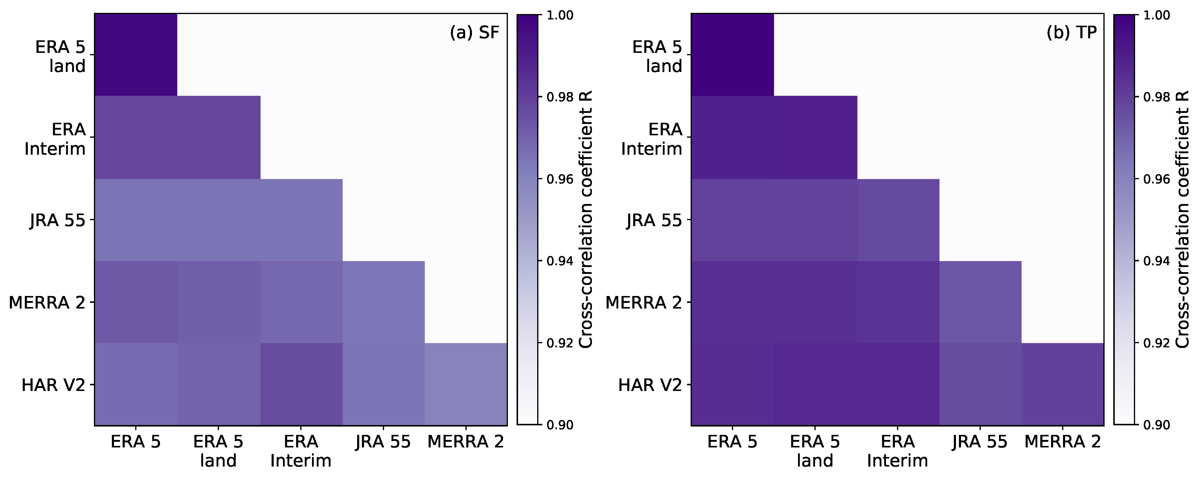
3.1. Cross-Correlation of the Reanalysis Data

The cross-correlation results of the TP and SF are shown in Figure 3. Overall, both analyses for TP and SF lead to acceptable results. The highest correlation regarding SF was found between ERA 5 and ERA 5 land with R = 0.99. All correlation coefficients vary between 0.96 and 0.99. The highest correlation coefficient regarding TP is met by several data pairs: ERA 5 and ERA 5 land, ERA 5 and ERA Interim, ERA 5 and HAR V2, ERA 5 land and ERA Interim, ERA land 5 and HAR V2. The lowest correlation coefficient with R = 0.96 was found between MERRA 2 and JRA 55.

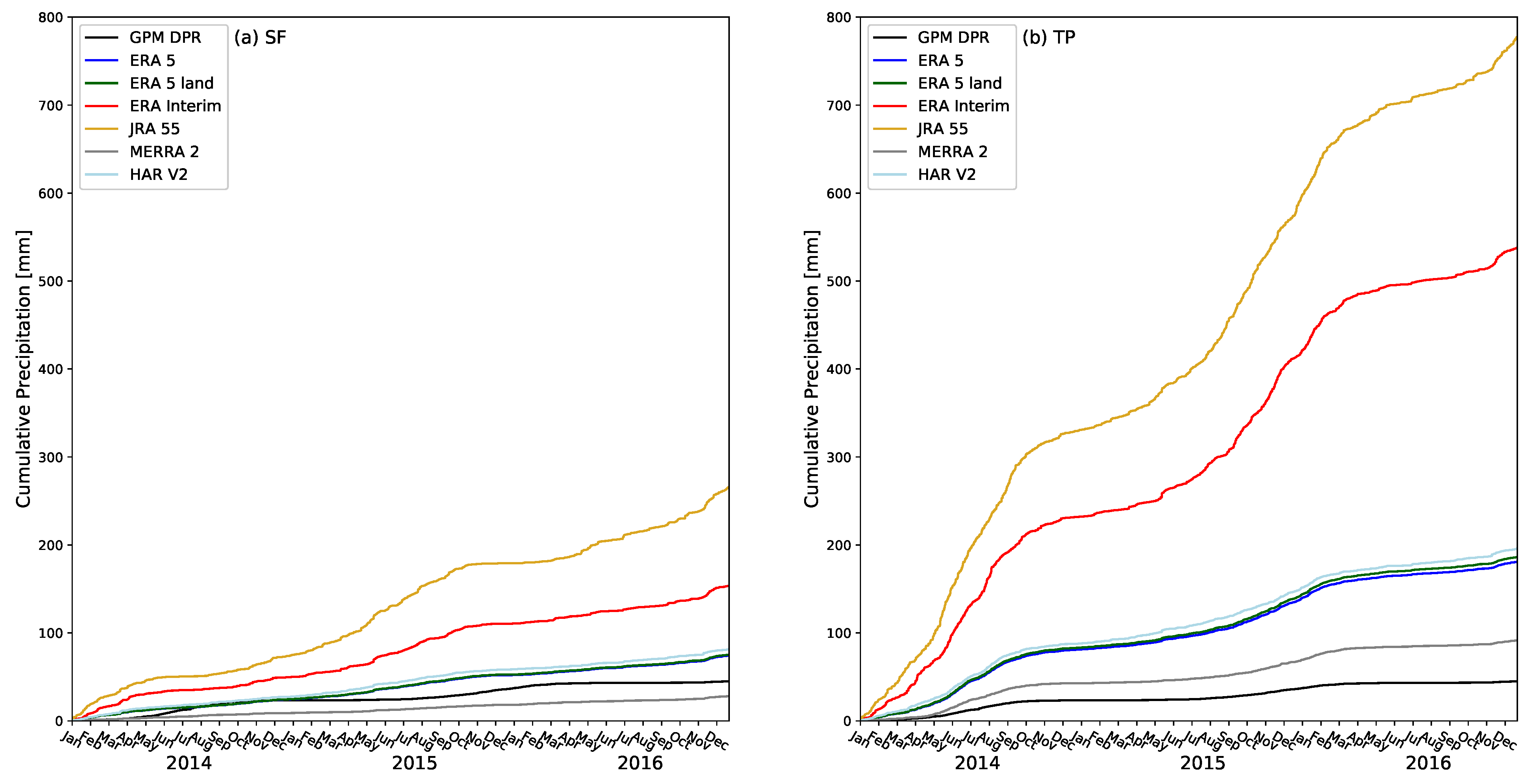
3.2. Comparison of the GPM DPR Data with Reanalysis Data

We compared the GPM DPR data with the reanalysis data to evaluate the quality of the GPM DPR data over the TiP. Figure 4 displays the spatial cumulative sum of (a) SF and (b) TP throughout the study period 2014–2016. We performed a Mann–Whitney U test to examine for the large differences in the cumulative sums of GPM DPR and the analysis data. The Mann–Whitney U test works on non-parametric data [27]. The null hypothesis is that the distribution of the data is the same as the distribution of the data to which it is compared. We tested all model-based data against GPM DPR and all model-based data against each other. We set the confidence level of 95% to reject the null hypothesis in favor of the alternative that the distributions are different. Based on the p-values, we reject the null hypothesis for all but one data pair and conclude that in all these cases, the distributions are significantly different. The exception builds ERA 5 SF with ERA 5 land SF. A p-value higher than 0.05 supports the null hypothesis, so ERA 5 SF and ERA 5 land SF have significantly the same distribution. Figure 4a also shows that there are no differences between ERA 5 and ERA 5 land in SF. We find that most of the precipitation occurs in the summer months (June, July, August) which can be seen in all TP data sets (Figure 4b). Hardly any differences can be seen in ERA 5 and ERA 5 land. Also, the accumulation line of HAR V2 is very close to ERA 5 and ERA 5 land. Wang et al. [23] found that snow depth in ERA 5 is overestimated in the region of the TiP, especially in winter and used JRA 55 data to correct snow depth in their data set HAR V2. MERRA 2 shows a very similar pattern compared to HAR V2, however the amount of precipitation is the lowest compared to all other data regarding SF. GPM DPR contains the lowest values for TP and is also comparable low regarding SF. We observe more TP in ERA Interim and JRA 55 compared to the other data. The differences become evident in the winter months when most of the data indicate lower TP. The overall patterns are also displayed in the SF data: we observe more SF in ERA Interim and JRA 55 compared to the other data. We monitor less SF in GPM DPR and MERRA 2.
Further, we analyzed the spatial patterns of TP and SF (Figure 5). We calculated the spatial per-grid-cell mean averaged over 2014–2016 for each of the precipitation products to better compare the data with each other. ERA 5, ERA 5 land and HAR V2 show the same pattern of TP. Compared to these data sets, GPM DPR and MERRA 2 show less TP, whereas ERA Interim and JRA 55 strongly observe more TP, especially in the northwestern parts of the study area, Pakistan and Tajikistan. ERA 5, ERA 5 land and GPM DPR SF show the same pattern of SF. MERRA 2 exhibits lower SF. ERA Interim, HAR V2 and especially JRA 55 illustrate a higher amount of SF, which is most prominent in the northwestern parts of the study area, Pakistan and Tajikistan.
In order to quantify the differences between the data sets, they are visualized in Figure 6 as bar plots. ERA 5, ERA 5 land and HAR V2 strongly agree regarding the precipitation amount relative to the amount of pixels for both SF and TP. MERRA 2 and GPM DPR illustrate the same proportion between TP and SF but with lower values. ERA Interim and JRA 55 both contain higher SF. This becomes more evident in the TP data.
Figure 7 displays the snowfall precipitation of the reanalysis data, GPM DPR SF, TP and the snowfall flags SSF, PNS and SSFPNS for the different regions (northwest, northeast, southwest, southeast) along various elevation levels (2500–3500 m until 5500–6500 m) in percent. Small color variations along the elevation levels or data sets indicate a high degree of agreement between the data sets. The differences are strongest between JRA 55 and MERRA 2 in the northwestern and southwestern TiP between JRA 55/HAR V2 and MERRA 2 in the range of 2500–3500 m and 4500–5500 m.

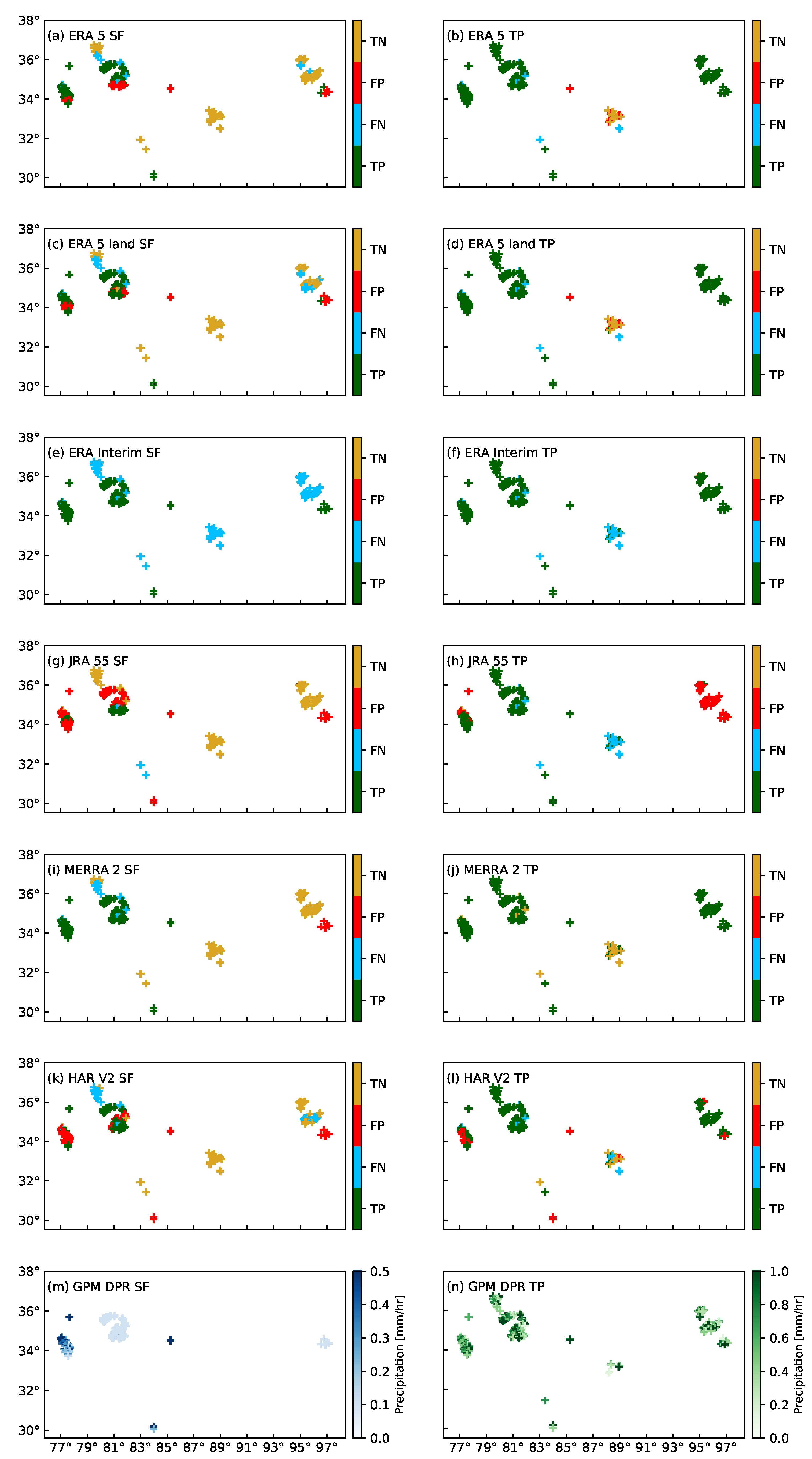
3.3. Intercomparison of GPM DPR and Reanalysis Data

First, the GPM DPR data were matched with the closest pixel and the closest time step of the reanalysis data to create a consistent data set for the intercomparison. It is well known that temporal or spatial mismatches between satellite and reanalysis data exist. To adress this issue, the intercomparison was performed for three different versions. We test whether a temporal or spatial adjustment contribute to a better intercomparison between the data. Therefore, the sections are: 3.3 closest pixel and time step, 3.4 closest pixel and temporal adjustment and 3.5 closest time step and spatial adjustment. This analysis was carried out in two steps: first, the snowfall flags (SSF, PNS and SSFPNS) were compared to the reanalysis data. Second, the GPM DPR TP and SF were compared to the reanalysis data. Since SF is of more relevance than TP in this study, the results of this intercomparison together with the results of the snowfall flags are shown in the following tables. In the following paragraphs, we mark the respective data sets in bold to highlight directly which data is being compared with each other.
First, the GPM DPR snowfall flags were compared to the total precipitation of the reanalysis data. This results in a homogeneous picture regarding the reanalyses data sets. There are hardly any differences in the results when the GPM DPR snowfall flags are compared to the TP reanalysis data. Overall, the POD and the PC are very high with a range from 0.63 to 0.94 (average around 0.8). However, the POFD is very high (around 0.8 on average) which indicates a strong bias in the GPM data. The FAR is very low with maximum values up to 0.16. The overall performance is represented by the HSS, which ranges between 0 for ERA Interim up to 0.16 for HAR V2. The results indicate that the GPM DPR snowfall flags are not well represented by the TP of the reanalysis data.
The intercomparison of the snowfall precipitation reanalysis with the GPM DPR snowfall flags displays similar results (Table A1) compared to the results of total precipitation against GPM DPR snowfall flags. The POD and PC range between 0.63 and 0.99 and the FAR is also very similar to the results of the intercomparison with the TP reanalyses with values between 0.01 and 0.19. The POFD shows similar high values compared to the intercomparison against the TP data. ERA Interim is the exception with a POFD of 0, which also results in an HSS of 0. The overall performance of the intercomparison of SF is better compared to the TP with an HSS of up to 0.48.
In addition, the results of the intercomparison of GPM DPR total precipitation against the total precipitation reanalysis data are described. The results are comparable to the intercomparison of the TP reanalysis data against the GPM DPR snowfall flags. POD and PC perform strong with values between 0.78 and 1 and FAR is low with values below 0.15. The POFD is remarkably high (0.39–1) and the HSS is 0.23 on average. The exception is ERA Interim with a POFD of 1 and an HSS of 0.
Table A2 displays the results of the intercomparison of the GPM DPR snow precipitation and the snow precipitation data of the reanalyses, and also for the temporal and spatial adjustment. As can be seen, POD and PC result in high values between 0.74 and 1 and the FAR is low (0.21 on average). The POFD is between 0.24 and 0.47. The HSS which ranges between 0.3 and 0.42. ERA Interim builds the exception with a POFD of 1 and the HSS of 0.
Figure 8 shows an example of the categorical scores for snowfall precipitation (Figure 8a,c,e,g,i,k) and total precipitation (Figure 8b,d,f,h,j,l) for all reanalyses data sets in comparison to the GPM DPR snowfall precipitation (Figure 8m) and total precipitation (Figure 8n) for 1–3 July 2014. SF values below 0.1 and above 0 were set to 0.1 for better visualization. Regarding SF the intercomparison of GPM DPR with the modeled data ERA 5, ERA 5 land, MERRA 2 and HAR V2 shows similar results: the occurrence of SF and no SF works well for lots of pixels; however, there are also lots of wrongs hits and misses. The results are different for ERA Interim and JRA 55. Whereas the detection of SF works for ERA Interim, lots of misses are detected as well. Regarding the comparison with JRA 55, the no SF detection works; however, lots of pixels result in wrong hits. The overall picture is very similar when regarding TP. However, the detection of SF works better compared to the detection of TP. ERA 5, ERA 5 land, JRA 55, MERRA 2 and HAR V2 draw also here a similar pattern. ERA Interim shows for TP also the same pattern compared to SF: GPM DPR is not well captured by ERA Interim regarding the true negatives.

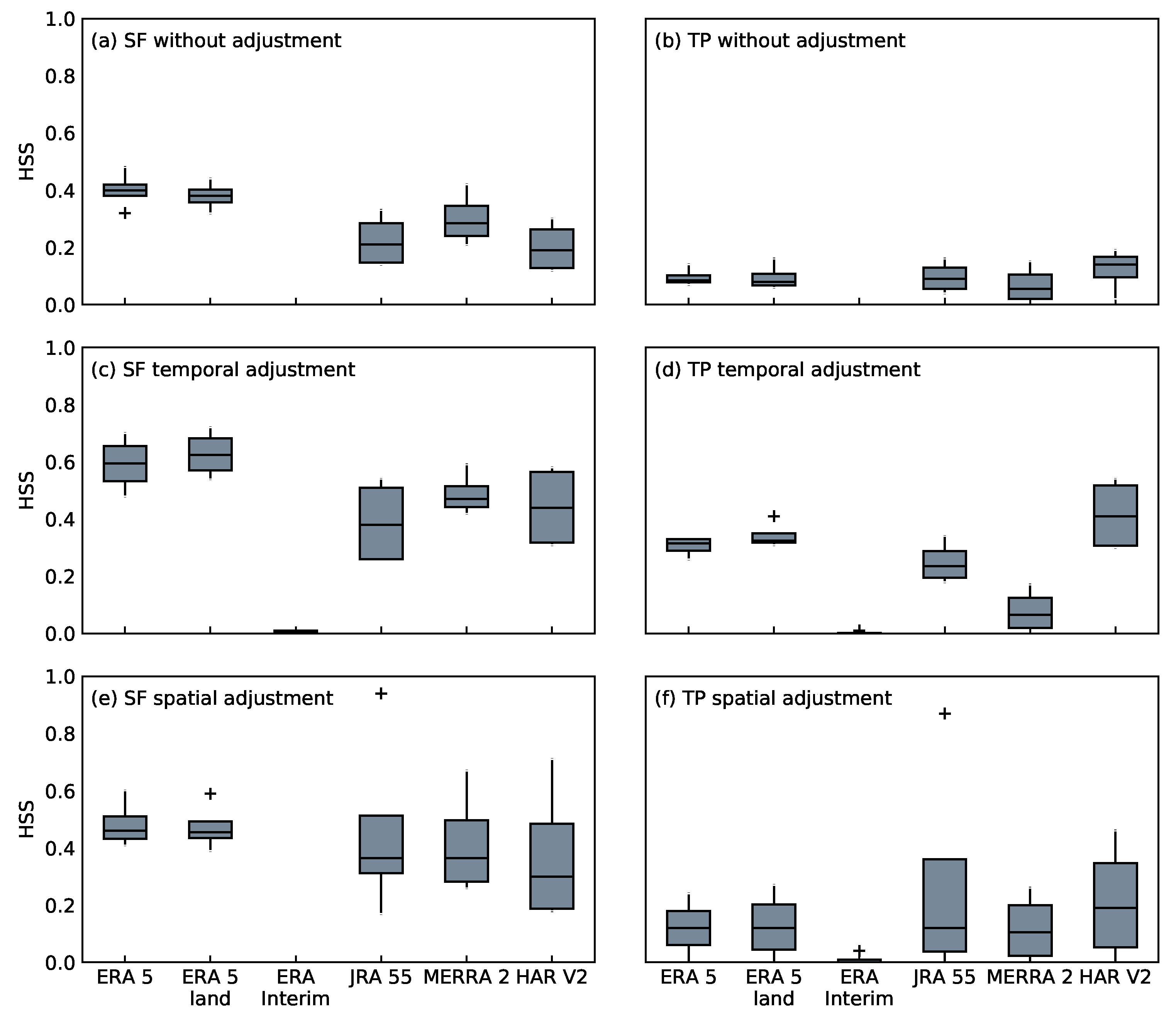
3.4. Comparing GPM DPR to Reanalysis Data with Temporal Adjustment

The GPM DPR data were matched with all reanalysis data which is +/−three hours away from the GPM DPR scan time and the closest pixel (Figure 2, bottom left). First, the results for the intercomparison of the GPM DPR snowfall flags with the total precipitation of the reanalysis data are analyzed. This approach highly impacts the POFD with lower values compared to the results without temporal adjustment. POD, FAR and PC are comparable to the results of the intercomparison of TP without temporal adjustment (range of POD and PC = 0.61–0.96, range of FAR = 0–0.09). Due to the strong improvement of the POFD, we also observe an improved HSS around 0.21 on average (mean HSS = 0.06 for the comparison without temporal adjustment). This approach highlights the differences between the GPM DPR snowfall flags: SSF performs better than PNS and the combination of both and is therefore better represented by the reanalysis data.
We also compared the GPM DPR snowfall flags to the snow precipitation of the reanalyses data. The results are shown in Table 2. The temporal adjustment of the data lead to a strong improvement of the intercomparison. The POFD was reduced remarkably, and the FAR slightly. POD and PC remain similar to the results without temporal adjustment (please compare Table A1 without the temporal adjustment to Table 2 with the temporal adjustment). The improvement of the POFD and FAR lead to stronger HSS between 0.26 and 0.72. The only exception is ERA Interim with an HSS of 0.01. This analysis also shows that the SSF snowfall flag matches the reanalyses data better compared to the PNS snowfall flag and the combination of both.
GPM DPR total precipitation was then compared to the reanalyses total precipitation data with the temporal adjustment of +/−three hours. In this analysis, the results of the intercomparison are improved due to a stronger POFD and similar results of POD, FAR and PC compared to the results without temporal adjustment. The improvement of the POFD is also reflected in stronger HSS values up to 0.54. As in the previous analyses, ERA Interim is the exception with an HSS of close to 0.
Further, we compared the GPM DPR snowfall precipitation to the snow precipitation of the reanalysis data. The results are shown in Table A2 in direct comparison to the results without temporal adjustment. The temporal adjustment improves the POFD. There are slight improvements in the results of POD, FAR and PC. The improvement due to the temporal adjustment is reflected in the HSS up to 0.59.

3.5. Intercomparison of GPM DPR and Reanalysis Data with Spatial Adjustment

A 3 × 3 pixel window around the GPM DPR data is used to match the reanalysis data (Figure 2, bottom right). Regarding the intercomparison of the GPM DPR snowfall flags against the total precipitation of the reanalysis data, the POD and the PC are very high between 0.71 and 1; however, the POFD is rather low for SSF (0.28 on average) and is very high regarding PNS and the combination of both at around 0.78 on average. The overall performance displayed in the HSS ranges between 0 and 0.31. The GPM snowfall flag SSF performs better compared to PNS and the combination of both.
The intercomparison of GPM DPR snowfall flags and the snowfall precipitation of the reanalyses is shown in Table A3. Please compare to Table A1 without spatial adjustment. It shows a high POD for all data sets (0.71–0.99). The POFD shows differences in the snowfall flags. The lowest POFD values can be observed for SSF and are higher for PNS and the combination of both flags. The FAR is low and the mean PC is 0.78. The HSS displays some differences in the GPM snowfall flags. Whereas ERA Interim shows no performance with an HSS of 0, SSF reaches up to 0.48 regarding ERA 5.
In a further analysis, GPM DPR total precipitation was compared to the reanalyses total precipitation data with the spatial adjustment of a 3 × 3 pixel window. POD is around 0.8 on average, FAR reaches a maximum 0.1 and PC ranges between 0.81 and 1. POFD is quite low with a maximum of 0.17. Exceptions are ERA Interim with a POFD of 1. JRA 55 is the only data set with an acceptable HSS of 0.87, whereas all other data sets result in values below 0.46.
In addition, GPM DPR snow precipitation was compared to the snowfall precipitation of the reanalyses data. The results are displayed in Table A2. POD ranges between 0.79 and 1, FAR reaches values between 0.01 and 0.19, PC is close to the optimal values (0.86–0.97), and POFD has a maximum of 0.07. It is notable that JRA 55 shows very good results with an HSS of 0.94 whereas ERA Interim in contrast does not align with the other reanalyses data. In contrast to the comparison of the reanalysis data against the GPM DPR snowfall flags, the comparison of the snowfall precipitation with the spatial adjustment also results in an improvement with a mean HSS of 0.59.
Figure 9 shows the distribution of the HSS which resulted from the intercomparison of SF and TP with the modeled data. It summarizes the overall performance: the temporal adjustment improves the HSS best and the spatial adjustment results in slight improvements.

4. Discussion

We did not use precipitation observation data for the intercomparison. The terrain of the TiP is very complex and orographic effects hinder the representativity of single observations. Comparing precipitation data over the TiP with a high spatio-temporal resolution is a challenge due to the sparse and unevenly distributed network of precipitation observation stations. Ali et al. [28] state that observation stations cover rather valleys. Even if available, precipitation observation data provide information on a daily basis. GPM DPR provides information on four overflights per day; however, this is insufficient for a valid comparison to daily observation data. In addition, depending on the swaths of GPM DPR it hits different areas of the TiP with its four overflights per day. This further limits the selection of precipitation observation data.
Snow from space can be observed using radar from the Cloud-Profiling Radar (CPR) onboard Cloudsat and the Global Precipitation Measurement Mission (GPM) dual-frequency precipitation radar (DPR). Cloudsat performs excellently in detecting and quantifying snowfall at high latitudes [29,30,31,32]. Due to the narrow swath of the CPR and the orbital frequency of Cloudsat, the frequent spatial and temporal monitoring of snowfall is limited. In addition, battery issues in 2011 made the satellite only operate at daytime only [33]. Further, Cloudsat provides snow precipitation over ocean and land, but rain precipitation is only available over ocean and not over land due to large uncertainties related to the heterogeneous surfaces, which complicate the retrieval of rain precipitation [34]. Several studies use Cloudsat CPR or the coincidence of Cloudsat and GPM for snow detection. In comparison to Cloudsat CPR, GPM DPR only detects 5–7% SF [29]. However, the authors point out that the differences in the radar sensitivity of Cloudsat and GPM must lead to large differences in the detection of SF. Furthermore, the coincidence data set of Cloudsat and GPM is only available at high latitudes, and thus, a comparison or combination of these data in this study over the TiP is therefore not possible [29,34]. In addition to its previously mentioned limitations, Cloudsat’s ability to capture precipitation on the surface attenuates during high-intensity precipitation events and thick clouds due to the W band radar [35,36]. It is not sensitive to light precipitation and underestimates light snow [36,37]. Uncertainties also occur in any near-surface precipitation, where ground interference impacts the quality of Cloudsat data especially in regions with high elevation and complex terrain [36,38]. In mid-latitude regions such as the TiP sample size of Cloudsat is reduced which also impacts its accuracy [38]. Validation studies are performed using Cloudsat at latitudes above 60° N. Studies that validate Cloudsat over regions such as the TiP do not exist which questions its performance in mid-latitudes.
Evaluation of data is critical when the ground truth has its own limitations. This is the case for observation stations, model-based data and satellite data. Therefore, conclusions that state that specific data sets outperform the ground truth data set need to be treated with caution. It is also important to note that differences in the evaluation occur when different temporal and spatial scales are evaluated [39]. Some studies compared various model-based and satellite-based snowfall precipitation products over the TiP. Tang et al. [40] conclude that reanalysis products tend to perform worse than satellite-based precipitation products that contain gauge adjustment in China, including the TiP. Bai et al. [41] compare multi-source blended data, reanalysis data and satellite data and sum up that the best quality data set for the TiP is a product that combines several sources of data. The comparison of ERA 5, ERA 5 land, ERA Interim and HAR over the TiP shows that ERA 5, ERA 5 land and HAR capture precipitation well, whereas the resolution of ERA Interim is too coarse to reproduce precipitation correctly [42]. This is especially evident in areas with high elevation and complex terrain compared to low elevated areas. A study conducted by [43] evaluates various gridded snowfall data sets using station observations over the TiP and they conclude that HAR performs better than ERA 5 and that a Chinese gridded near-surface meteorological data set consisting of remote sensing data, reanalysis data and observations performs best among the compared data sets. An intercomparison of model-based and satellite-based precipitation data sets over a sub-region of the central Himalaya and the southwestern TiP conducted by [44] concludes that extreme precipitation is better captured by high resolution data and that the use of precipitation data set should be selected according to its research question.

5. Conclusions

We have examined the performance of GPM DPR (snowfall flags, snowfall precipitation and total precipitation) with well-known reanalysis data used as ground truth. The promising results of the cross-correlation among the reanalysis data proofs its strong performance on the TiP. The intercomparison of the GPM DPR snowfall flags performs poorly when compared directly to the reanalysis data, and the spatial adjustment does not improve the intercomparison results significantly. However, we showed the temporal adjustment of three hours between the GPM DPR snowfall flags and reanalysis data leads to promising results. The intercomparison of the GPM DPR total precipitation and snowfall precipitation against reanalysis data lead to promising results and we examined an improvement of the results by the use of the temporal and spatial adjustment. In summary, we show that GPM DPR Level 2A does not match the reanalysis data well and that temporal and spatial adjustments might help to improve the results. In general, this is in agreement with studies from [45,46,47] which state that mismatches between satellite and reanalysis data exist. We recommend that when using data from different sources such as model data and satellite data, a check should first be made to determine whether there is a spatial and/or temporal offset before the data are combined and blended. Satellite remote sensing offers great potential to map precipitation on a large temporal and spatial scale. The analysis of GPM DPR data generally shows that mapping SF is also possible from space. However, satellite missions such as GPM need to improve the quality of SF data to match or exceed the quality of model-based SF data.

Author Contributions

Conceptualization, C.K., B.T. and J.B.; methodology, C.K., B.T. and J.B.; software, C.K.; validation, C.K.; formal analysis, C.K.; investigation, C.K., B.T. and J.B.; resources, J.B.; data curation, C.K.; writing—original draft preparation, C.K.; writing—review and editing, C.K., B.T. and J.B.; visualization, C.K.; supervision, B.T. and J.B.; project administration, B.T. and J.B.; funding acquisition, B.T. and J.B. All authors have read and agreed to the published version of the manuscript.

Funding

This study was conducted within the project “Precipitation patterns, snow and glacier response in High Asia and their variability on sub-decadal time scales—Remote Sensing of precipitation” (prime-RS), which is funded by the German Research Foundation (DFG projects: BE1780/46-1 and TH1531/6-1). The first author also received funding from the MArburg University Research Academy (MARA) final scholarship.

Data Availability Statement

No new data were created or analyzed in this study. Data sharing is not applicable to this article.

Acknowledgments

We kindly thank the three anonymous reviewers for their helpful suggestions on a previous version of this manuscript.

Conflicts of Interest

The authors declare no conflicts of interest. The funders had no role in the design of the study; in the collection, analyses, or interpretation of data; in the writing of the manuscript; or in the decision to publish the results.

Abbreviations

The following abbreviations are used in this manuscript:
DPRDual-frequency precipitation radar
ERA 5ECMWF Reanalysis v5
ERA 5 landECMWF Reanalysis v5 land
ERA InterimECMWF Reanalysis - Interim
FARFalse alarm rate
FNFalse negative
FPFalse positive
GPMGlobal Precipitation Measurement Mission
HAR V2High Asia Refined analysis version 2
HSSHeidke skill score
IMERGIntegrated Multi-satellitE Retrievals for GPM
JRA 55Japanese 55-year Reanalysis
MERRA 2Modern-Era Retrospective analysis for Research and Applications, Version 2
MSMatched scan
NEXRADNext Generation Radar
PCPercentage correct
PLPPProbability of liquid precipitation phase
PODProbability of detection
POFDProbability of false detection
PNSPhase near surface
SFSnowfall precipitation
SSFSurface snowfall flag
SSFPNSLowest common denominator of SSF and PNS
TiPTibetan Plateau
TNTrue negative
TPTrue positive
TPTotal precipitation

Appendix A

Table A1. Validation metrics calculated between GPM DPR SSF/PNS/SSFPNS and snow precipitation of reanalysis data sets.
Snow Precipitation
ERA 5ERA 5 LandERA InterimJRA 55MERRA 2HAR V2Optimal Value
GPMPOD0.72/0.98/0.990.72/0.98/0.980.63/0.93/0.930.77/0.99/0.990.74/0.97/0.980.74/0.97/0.971
DPRPOFD0.31/0.68/0.610.31/0.70/0.640.0/0.0/0.00.50/0.86/0.850.41/0.82/0.790.49/0.87/0.860
SSFFAR0.10/0.11/0.090.1/0.12/0.100.0/0.0/0.00.41/0.41/0.40.21/0.22/0.200.33/0.33/0.330
PNSHSS0.32/0.40/0.480.32/0.37/0.440.0/0.0/0.00.27/0.14/0.150.32/0.21/0.250.25/0.12/0.131
SSFPNSPC0.71/0.88/0.900.71/0.87/0.890.63/0.93/0.930.63/0.61/0.620.69/0.78/0.790.64/0.67/0.681
Table A2. Validation metrics calculated between GPM DPR snow precipitation and snow precipitation of reanalysis data sets without adjustment, temporal adjustment and spatial adjustment.
Snow Precipitation
ERA 5ERA 5 LandERA InterimJRA 55MERRA 2HAR V2Optimal Value
GPMPOD0.750.741.00.810.780.761
DPRPOFD0.240.261.00.480.340.470
SFFAR0.080.090.190.380.180.310
withoutHSS0.400.390.00.330.420.301
adjustmentPC0.750.740.810.660.740.661
GPMPOD0.770.780.610.890.820.861
DPRPOFD0.110.100.00.350.200.290
SFFAR0.040.040.00.290.110.210
temporalHSS0.550.580.010.540.590.581
adjustmentPC0.800.810.610.770.810.791
GPMPOD0.80.791.01.00.820.841
DPRPOFD0.040.041.00.070.050.050
SFFAR0.010.010.190.040.020.020
spatialHSS0.600.590.00.940.670.711
adjustmentPC0.830.830.810.970.860.871
Table A3. Validation metrics calculated between GPM DPR SSF/PNS/SSFPNS and snow precipitation of reanalysis data sets with the spatial adjustment of the 3 × 3 pixel window.
Snow Precipitation
ERA 5ERA 5 LandERA InterimJRA 55MERRA 2HAR V2Optimal Value
GPMPOD0.78/0.98/0.990.78/0.98/0.980.71/0.92/0.930.80/0.99/0.810.79/0.97/0.970.79/0.97/0.971
DPRPOFD0.27/0.66/0.610.26/0.67/0.620.0/0.0/0.00.45/0.84/0.450.32/0.77/0.750.39/0.82/0.820
SSFFAR0.09/0.14/0.110.09/0.14/0.110.0/0.0/0.00.34/0.39/0.330.15/0.20/0.180.25/0.30/0.300
PNSHSS0.44/0.41/0.480.45/0.39/0.460.0/0.0/0.00.36/0.17/0.370.44/0.26/0.290.41/0.18/0.191
SSFPNSPC0.77/0.86/0.890.77/0.86/0.880.71/0.92/0.930.68/0.64/0.690.76/0.79/0.810.72/0.70/0.701

References

  1. Luo, J.; Chen, H.; Zhou, B. Comparison of Snowfall Variations over China Identified from Different Snowfall/Rainfall Discrimination Methods. J. Meteorol. Res. 2020, 34, 1114–1128. [Google Scholar] [CrossRef]
  2. Rysman, J.F.; Panegrossi, G.; Sanò, P.; Marra, A.; Dietrich, S.; Milani, L.; Kulie, M. SLALOM: An All-Surface Snow Water Path Retrieval Algorithm for the GPM Microwave Imager. Remote Sens. 2018, 10, 1278. [Google Scholar] [CrossRef]
  3. Le, M.; Chandrasekar, V. Ground Validation of Surface Snowfall Algorithm in GPM Dual-Frequency Precipitation Radar. J. Atmos. Ocean. Technol. 2019, 36, 607–619. [Google Scholar] [CrossRef]
  4. Wang, Y.; Broxton, P.; Fang, Y.; Behrangi, A.; Barlage, M.; Zeng, X.; Niu, G. A Wet-Bulb Temperature-Based Rain-Snow Partitioning Scheme Improves Snowpack Prediction over the Drier Western United States. Geophys. Res. Lett. 2019, 46, 13825–13835. [Google Scholar] [CrossRef]
  5. Dong, W.; Lin, Y.; Wright, J.S.; Xie, Y.; Xu, F.; Yang, K.; Li, X.; Tian, L.; Zhao, X.; Cao, D. Connections Between a Late Summer Snowstorm Over the Southwestern Tibetan Plateau and a Concurrent Indian Monsoon Low-Pressure System. J. Geophys. Res. Atmos. 2018, 123, 13676–13691. [Google Scholar] [CrossRef]
  6. Foufoula-Georgiou, E.; Guilloteau, C.; Nguyen, P.; Aghakouchak, A.; Hsu, K.L.; Busalacchi, A.; Turk, F.J.; Peters-Lidard, C.; Oki, T.; Duan, Q.; et al. Advancing Precipitation Estimation, Prediction, and Impact Studies. Bull. Am. Meteorol. Soc. 2020, 101, E1584–E1592. [Google Scholar] [CrossRef]
  7. Takbiri, Z.; Ebtehaj, A.; Foufoula-Georgiou, E.; Kirstetter, P.E.; Turk, F.J. A Prognostic Nested k-Nearest Approach for Microwave Precipitation Phase Detection over Snow Cover. J. Hydrometeorol. 2019, 20, 251–274. [Google Scholar] [CrossRef] [PubMed]
  8. Kolbe, C.; Thies, B.; Turini, N.; Liu, Z.; Bendix, J. Precipitation Retrieval over the Tibetan Plateau from the Geostationary Orbit—Part 2: Precipitation Rates with Elektro-L2 and Insat-3D. Remote Sensing 2020, 12, 2114. [Google Scholar] [CrossRef]
  9. Skofronick-Jackson, G.; Petersen, W.; Hudak, D.; Schwaller, M. GPM Cold-Season Precipitation Experiment (GCPEx). 2012; p. 34. Available online: https://gpm.nasa.gov/sites/default/files/document_files/GCPEx_science_plan_CURRENT.pdf (accessed on 15 November 2022).
  10. Liao, L.; Meneghini, R. A Study on the Feasibility of Dual-Wavelength Radar for Identification of Hydrometeor Phases. J. Appl. Meteorol. Climatol. 2011, 50, 449–456. [Google Scholar] [CrossRef]
  11. Iguchi, T.; Seto, S.; Meneghini, R.; Yoshida, N.; Awaka, J.; Le, M.; Chandrasekar, V.; Brodzik, S.; Kubota, T. GPM/DPR Level-2 Algorithm Theoretical Basis Document. 2018; p. 127. Available online: https://gpm.nasa.gov/sites/default/files/2022-06/ATBD_DPR_V07A.pdf (accessed on 15 November 2022).
  12. Petracca, M.; D’Adderio, L.P.; Porcù, F.; Vulpiani, G.; Sebastianelli, S.; Puca, S. Validation of GPM Dual-Frequency Precipitation Radar (DPR) Rainfall Products over Italy. J. Hydrometeorol. 2018, 19, 907–925. [Google Scholar] [CrossRef]
  13. Speirs, P.; Gabella, M.; Berne, A. A Comparison between the GPM Dual-Frequency Precipitation Radar and Ground-Based Radar Precipitation Rate Estimates in the Swiss Alps and Plateau. J. Hydrometeorol. 2017, 18, 1247–1269. [Google Scholar] [CrossRef]
  14. Le, M.; Chandrasekar, V.; Biswas, S. An Algorithm to Identify Surface Snowfall from GPM DPR Observations. IEEE Trans. Geosci. Remote Sens. 2017, 55, 4059–4071. [Google Scholar] [CrossRef]
  15. Kubota, T.; Seto, S.; Satoh, M.; Nasuno, T.; Iguchi, T.; Masaki, T.; Kwiatkowski, J.M.; Oki, R. Cloud Assumption of Precipitation Retrieval Algorithms for the Dual-Frequency Precipitation Radar. J. Atmos. Ocean. Technol. 2020, 37, 2015–2031. [Google Scholar] [CrossRef]
  16. Seto, S.; Iguchi, T.; Meneghini, R.; Awaka, J.; Kubota, T.; Masaki, T.; Takahashi, N. The Precipitation Rate Retrieval Algorithms for the GPM Dual-frequency Precipitation Radar. J. Meteorol. Soc. Jpn. Ser. II 2021, 99, 205–237. [Google Scholar] [CrossRef]
  17. Skofronick-Jackson, G.; Kulie, M.; Milani, L.; Munchak, S.J.; Wood, N.B.; Levizzani, V. Satellite Estimation of Falling Snow: A Global Precipitation Measurement (GPM) Core Observatory Perspective. J. Appl. Meteorol. Climatol. 2019, 58, 1429–1448. [Google Scholar] [CrossRef]
  18. Sims, E.M.; Liu, G. A Parameterization of the Probability of Snow–Rain Transition. J. Hydrometeorol. 2015, 16, 1466–1477. [Google Scholar] [CrossRef]
  19. Dee, D.P.; Uppala, S.M.; Simmons, A.J.; Berrisford, P.; Poli, P.; Kobayashi, S.; Andrae, U.; Balmaseda, M.A.; Balsamo, G.; Bauer, P.; et al. The ERA-Interim reanalysis: Configuration and performance of the data assimilation system. Q. J. R. Meteorol. Soc. 2011, 137, 553–597. [Google Scholar] [CrossRef]
  20. Hersbach, H.; Bell, B.; Berrisford, P.; Hirahara, S.; Horányi, A.; Muñoz-Sabater, J.; Nicolas, J.; Peubey, C.; Radu, R.; Schepers, D.; et al. The ERA5 global reanalysis. Q. J. R. Meteorol. Soc. 2020, 146, 1999–2049. [Google Scholar] [CrossRef]
  21. Kobayashi, S.; Ota, Y.; Harada, Y.; Ebita, A.; Moriya, M.; Onoda, H.; Onogi, K.; Kamahori, H.; Kobayashi, C.; Endo, H.; et al. The JRA-55 Reanalysis: General Specifications and Basic Characteristics. J. Meteorol. Soc. Jpn. Ser. II 2015, 93, 5–48. [Google Scholar] [CrossRef]
  22. Gelaro, R.; McCarty, W.; Suárez, M.J.; Todling, R.; Molod, A.; Takacs, L.; Randles, C.A.; Darmenov, A.; Bosilovich, M.G.; Reichle, R.; et al. The Modern-Era Retrospective Analysis for Research and Applications, Version 2 (MERRA-2). J. Clim. 2017, 30, 5419–5454. [Google Scholar] [CrossRef]
  23. Wang, X.; Tolksdorf, V.; Otto, M.; Scherer, D. WRF-based dynamical downscaling of ERA5 reanalysis data for High Mountain Asia: Towards a new version of the High Asia Refined analysis. Int. J. Climatol. 2021, 41, 743–762. [Google Scholar] [CrossRef]
  24. Mekonnen, K.; Melesse, A.M.; Woldesenbet, T.A. Effect of temporal sampling mismatches between satellite rainfall estimates and rain gauge observations on modelling extreme rainfall in the Upper Awash Basin, Ethiopia. J. Hydrol. 2021, 598, 126467. [Google Scholar] [CrossRef]
  25. Urraca, R.; Lanconelli, C.; Gobron, N. Impact of the Spatio-Temporal Mismatch Between Satellite and In Situ Measurements on Validations of Surface Solar Radiation. J. Geophys. Res. Atmos. 2024, 129, e2024JD041007. [Google Scholar] [CrossRef]
  26. World Weather Research Program/Working Group on Numerical Experimentation Joint Working Group on Verification. Forecast Verification—Issues, Methods and FAQ. Available online: https://www.cawcr.gov.au/projects/verification/ (accessed on 30 September 2022).
  27. Mann, H.B.; Whitney, D.R. On a Test of Whether one of Two Random Variables is Stochastically Larger than the Other. Ann. Math. Stat. 1947, 18, 50–60. [Google Scholar] [CrossRef]
  28. Ali, S.; Chen, Y.; Azmat, M.; Kayumba, P.M.; Ahmed, Z.; Mind’je, R.; Ghaffar, A.; Qin, J.; Tariq, A. Long-Term Performance Evaluation of the Latest Multi-Source Weighted-Ensemble Precipitation (MSWEP) over the Highlands of Indo-Pak (1981–2009). Remote Sens. 2022, 14, 4773. [Google Scholar] [CrossRef]
  29. Casella, D.; Panegrossi, G.; Sanò, P.; Marra, A.C.; Dietrich, S.; Johnson, B.T.; Kulie, M.S. Evaluation of the GPM-DPR snowfall detection capability: Comparison with CloudSat-CPR. Atmos. Res. 2017, 197, 64–75. [Google Scholar] [CrossRef]
  30. Haynes, J.M.; L’Ecuyer, T.S.; Stephens, G.L.; Miller, S.D.; Mitrescu, C.; Wood, N.B.; Tanelli, S. Rainfall retrieval over the ocean with spaceborne W-band radar. J. Geophys. Res. Atmos. 2009, 114, 2008JD009973. [Google Scholar] [CrossRef]
  31. Liu, G. Deriving snow cloud characteristics from CloudSat observations. J. Geophys. Res. Atmos. 2008, 113, 2007JD009766. [Google Scholar] [CrossRef]
  32. Wood, N.B.; L’Ecuyer, T.S.; Heymsfield, A.J.; Stephens, G.L.; Hudak, D.R.; Rodriguez, P. Estimating snow microphysical properties using collocated multisensor observations. J. Geophys. Res. Atmos. 2014, 119, 8941–8961. [Google Scholar] [CrossRef]
  33. Edel, L.; Rysman, J.F.; Claud, C.; Palerme, C.; Genthon, C. Potential of Passive Microwave around 183 GHz for Snowfall Detection in the Arctic. Remote Sens. 2019, 11, 2200. [Google Scholar] [CrossRef]
  34. Tang, G.; Long, D.; Behrangi, A.; Wang, C.; Hong, Y. Exploring Deep Neural Networks to Retrieve Rain and Snow in High Latitudes Using Multisensor and Reanalysis Data. Water Resour. Res. 2018, 54, 8253–8278. [Google Scholar] [CrossRef]
  35. Hudak, D.; Rodriguez, P.; Donaldson, N. Validation of the CloudSat precipitation occurrence algorithm using the Canadian C band radar network. J. Geophys. Res. Atmos. 2008, 113, 2008JD009992. [Google Scholar] [CrossRef]
  36. King, F.; Fletcher, C.G. Using CloudSat-Derived Snow Accumulation Estimates to Constrain Gridded Snow Water Equivalent Products. Earth Space Sci. 2021, 8, e2021EA001835. [Google Scholar] [CrossRef]
  37. Stephens, G.L.; Vane, D.G.; Boain, R.J.; Mace, G.G.; Sassen, K.; Wang, Z.; Illingworth, A.J.; O’connor, E.J.; Rossow, W.B.; Durden, S.L.; et al. The Cloudsat Mission and the A-Train: A New Dimension of Space-Based Observations of Clouds and Precipitation. Bull. Am. Meteorol. Soc. 2002, 83, 1771–1790. [Google Scholar] [CrossRef]
  38. King, F.; Fletcher, C.G. Using CloudSat-CPR Retrievals to Estimate Snow Accumulation in the Canadian Arctic. Earth Space Sci. 2020, 7, e2019EA000776. [Google Scholar] [CrossRef]
  39. Sun, S.; Shi, W.; Zhou, S.; Chai, R.; Chen, H.; Wang, G.; Zhou, Y.; Shen, H. Capacity of Satellite-Based and Reanalysis Precipitation Products in Detecting Long-Term Trends across Mainland China. Remote Sens. 2020, 12, 2902. [Google Scholar] [CrossRef]
  40. Tang, G.; Clark, M.P.; Papalexiou, S.M.; Ma, Z.; Hong, Y. Have satellite precipitation products improved over last two decades? A comprehensive comparison of GPM IMERG with nine satellite and reanalysis datasets. Remote Sens. Environ. 2020, 240, 111697. [Google Scholar] [CrossRef]
  41. Bai, L.; Wen, Y.; Shi, C.; Yang, Y.; Zhang, F.; Wu, J.; Gu, J.; Pan, Y.; Sun, S.; Meng, J. Which Precipitation Product Works Best in the Qinghai-Tibet Plateau, Multi-Source Blended Data, Global/Regional Reanalysis Data, or Satellite Retrieved Precipitation Data? Remote Sens. 2020, 12, 683. [Google Scholar] [CrossRef]
  42. Chen, Y.; Sharma, S.; Zhou, X.; Yang, K.; Li, X.; Niu, X.; Hu, X.; Khadka, N. Spatial performance of multiple reanalysis precipitation datasets on the southern slope of central Himalaya. Atmos. Res. 2021, 250, 105365. [Google Scholar] [CrossRef]
  43. Sun, F.; Chen, Y.; Li, Y.; Duan, W.; Li, B.; Fang, G.; Li, Z. Evaluation of multiple gridded snowfall datasets using gauge observations over high mountain Asia. J. Hydrol. 2023, 626, 130346. [Google Scholar] [CrossRef]
  44. Hamm, A.; Arndt, A.; Kolbe, C.; Wang, X.; Thies, B.; Boyko, O.; Reggiani, P.; Scherer, D.; Bendix, J.; Schneider, C. Intercomparison of Gridded Precipitation Datasets over a Sub-Region of the Central Himalaya and the Southwestern Tibetan Plateau. Water 2020, 12, 3271. [Google Scholar] [CrossRef]
  45. Feng, F.; Wang, K. Merging Satellite Retrievals and Reanalyses to Produce Global Long-Term and Consistent Surface Incident Solar Radiation Datasets. Remote Sens. 2018, 10, 115. [Google Scholar] [CrossRef]
  46. Yang, D. Quantifying the spatial scale mismatch between satellite-derived solar irradiance and Situ Meas. A Case Study Using CERES Synop. Surf. Shortwave Flux Oklahoma Mesonet. J. Renew. Sustain. Energy 2020, 12, 056104. [Google Scholar] [CrossRef]
  47. Qin, Y.; McVicar, T.R.; Huang, J.; West, S.; Steven, A.D. On the validity of using ground-based observations to validate geostationary-satellite-derived direct and diffuse surface solar irradiance: Quantifying the spatial mismatch and temporal averaging issues. Remote Sens. Environ. 2022, 280, 113179. [Google Scholar] [CrossRef]
Figure 1. Overview of (a) the number of pixels for surface snowfall flag (SSF), phase near surface (PNS) and the combination of both (SSFPNS) delineated in snow precipitation and no snow precipitation and (b) the spatial distribution of GPM overflights over the TiP relative to the number of available scenes (2014–2016).
Atmosphere 15 01076 g001
Figure 2. Overview of the processing scheme for the intercomparison of the GPM DPR data. TP = total precipitation, SF = snowfall precipitation, SSF = surface snowfall flag, PNS = phase near surface, PLPP = probability of liquid precipitation phase.
Atmosphere 15 01076 g002
Figure 3. Results of the cross-correlation coefficient R (Spearman correlation) between (a) the snowfall precipitation and (b) total precipitation reanalysis data sets for all scenes. All correlations are statistically significant at the 99% confidence interval.
Atmosphere 15 01076 g003
Figure 4. Spatial cumulative sum of GPM DPR and reanalysis data adjusted to GPM’s 5 km resolution of (a) snow precipitation and (b) total precipitation from each available common time step throughout the study period 2014–2016.
Atmosphere 15 01076 g004
Figure 5. Spatial per-grid-cell frequency averaged over 2014–2016 for each of the precipitation products on the TiP.
Atmosphere 15 01076 g005
Figure 6. Average total precipitation and snowfall precipitation of reanalysis and GPM DPR data per time step throughout the period 2014–2016. The bars indicate the mean total precipitation and mean snowfall precipitation over the TiP, calculated by dividing the sum of total precipitation and snowfall precipitation by the number of time steps and the number of pixels of the precipitating area. The different colours represent each data set.
Atmosphere 15 01076 g006
Figure 7. Percentage distribution of the GPM DPR snowfall flags (SSF, PNS, SSF & PNS) and reanalysis pixels along elevation levels based on different regions of the TiP. The colour intensity indicates the similarity to other data and elevation levels. Our study is restricted to High Mountain Asia (65° E–105° E, 25° N–45° N) with the shape of the TiP and an elevation > 2500 m.
Atmosphere 15 01076 g007
Figure 8. Example of the categorical scores for the intercomparison of GPM DPR SF and TP with all reanalyses data sets (SF, TP) for 1–3 July 2014.
Atmosphere 15 01076 g008
Figure 9. Boxplots of the HSS as the result of the intercomparison between the GPM DPR snowfall flags, snowfall precipitation and total precipitation with snowfall precipitation (a,c,e) and total precipitation (b,d,f) of the reanalysis data. Crosses mark outliers.
Atmosphere 15 01076 g009
Table 1. Overview of the GPM and reanalysis data.
Data SetSub Data SetSpatial ResolutionTemporal ResolutionSource
GPM DPR (Level 2A) (Global Precipitation Measurement Mission Dual-Frequency Precipitation Radar)total precipitation, snowfall precipitation, snowfall flags (SSF, PNS, SSFPNS)5 km (swath width 245 km)1.5 h (March 2014–near real time)PPS NASA (2022) https://gpm.nasa.gov/data/directory accessed on 15 November 2022.
GPM IMERG (Level 3, Final Run) (GPM Integrated Multi-satellitE Retrievals for GPM)probability of liquid precipitation phase11 km (global)30 min (March 2014–near real time)PPS NASA (2019) https://gpm.nasa.gov/data/directory accessed on 15 November 2022.
ERA 5 (ECMWF Reanalysis v5)total precipitation, snowfall precipitation30 km (global)1 h (1979–near real time)Service, C.C.C. (2019) European Centre for Medium-Range Weather Forecasts https://cds.climate.copernicus.eu/ accessed on 15 November 2022.
ERA 5 land (ECMWF Reanalysis v5 land)total precipitation, snowfall precipitation9 km (global)1 h (1981–near real time)[19] European Centre for Medium-Range Weather Forecasts https://cds.climate.copernicus.eu/ accessed on 15 November 2022.
ERA Interim (ECMWF Reanalysis—Interim)total precipitation, snowfall precipitation80 km (global)3 h (1979–August 2019)[20] European Centre for Medium-Range Weather Forecasts https://www.wdc-climate.de/ui/project?acronym=ERA_INTERIM accessed on 15 November 2022.
JRA 55 (Japanese 55-year Reanalysis)total precipitation, snowfall precipitation55 km (global)6 h (1958–near real time)[21] Japan Meteorological Agency https://rda.ucar.edu/datasets/ds628-0/ accessed on 15 November 2022.
MERRA 2 (Modern-Era Retrospective analysis for Research and Applications, Version 2)total precipitation, snowfall precipitation55 × 69 km (global)1 h (1980–near real time)[22] NASA’s Global Modeling and Assimilation Office https://disc.gsfc.nasa.gov/ accessed on 15 November 2022.
HAR V2 (High Asia Refined analysis version 2)total precipitation, snowfall precipitation10 km (High Mountain Asia)1 h (2004–2018)[23] https://data.klima.tu-berlin.de/HAR/v2/d10km/d/2d/ accessed on 15 November 2022
Table 2. Validation metrics calculated between GPM DPR SSF/PNS/SSFPNS and snow precipitation of reanalysis data sets with the temporal adjustment of +/−3 h.
Snow Precipitation
ERA 5ERA 5 LandERA InterimJRA 55MERRA 2HAR V2Optimal Value
GPMPOD0.75/0.98/0.980.77/0.98/0.990.61/0.93/0.930.86/0.99/1.00.78/0.98/0.980.86/0.99/0.991
DPRPOFD0.12/0.41/0.350.10/0.38/0.330.0/0.0/1.00.37/0.79/0.780.24/0.66/0.630.30/0.75/0.750
SSFFAR0.04/0.04/0.040.04/0.39/0.030.0/0.0/0.00.29/0.28/0.280.11/0.12/0.110.21/0.20/0.200
PNSHSS0.48/0.64/0.700.54/0.67/0.720.01/0.01/0.00.5/0.26/0.260.49/0.42/0.450.56/0.31/0.321
SSFPNSPC0.78/0.94/0.950.80/0.95/0.960.61/0.93/0.930.75/0.74/0.740.77/0.87/0.880.79/0.80/0.801
Disclaimer/Publisher’s Note: The statements, opinions and data contained in all publications are solely those of the individual author(s) and contributor(s) and not of MDPI and/or the editor(s). MDPI and/or the editor(s) disclaim responsibility for any injury to people or property resulting from any ideas, methods, instructions or products referred to in the content.

