


Assessment of Numerical Forecasts for Hub-Height Wind Resource Parameters during an Episode of Significant Wind Speed Fluctuations

 ,
,
Abstract
:1. Introduction
2. Models and Methods
2.1. M-O Similarity Theory (ST) Method
2.2. Wind Farm Parameterization (WFP) Method
2.3. NWP Models and Scenarios Setup
2.4. Wind Farm Observation Data
3. Results and Discussions
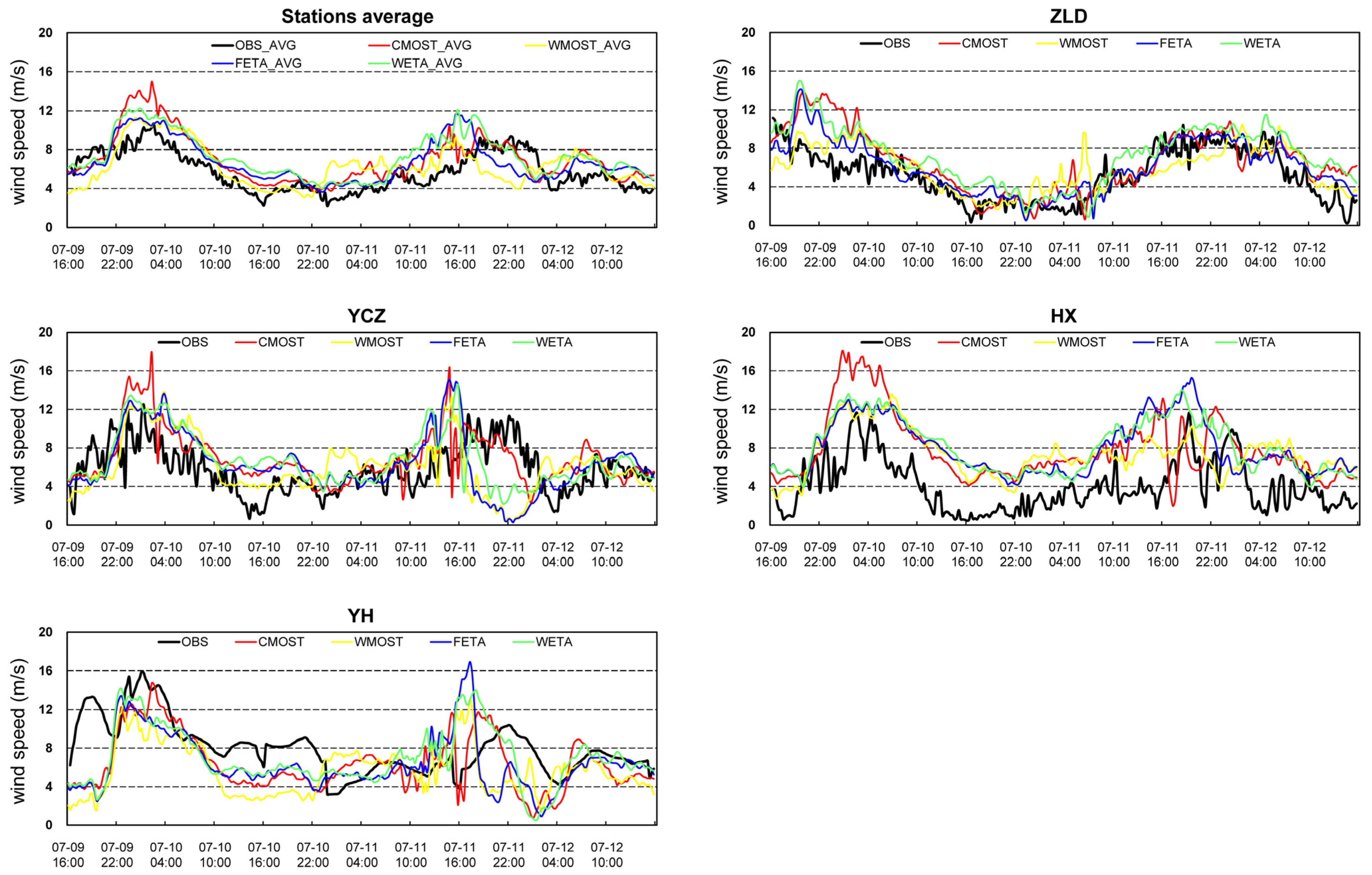
3.1. Comparative Forecast Evaluation of Different Scenario
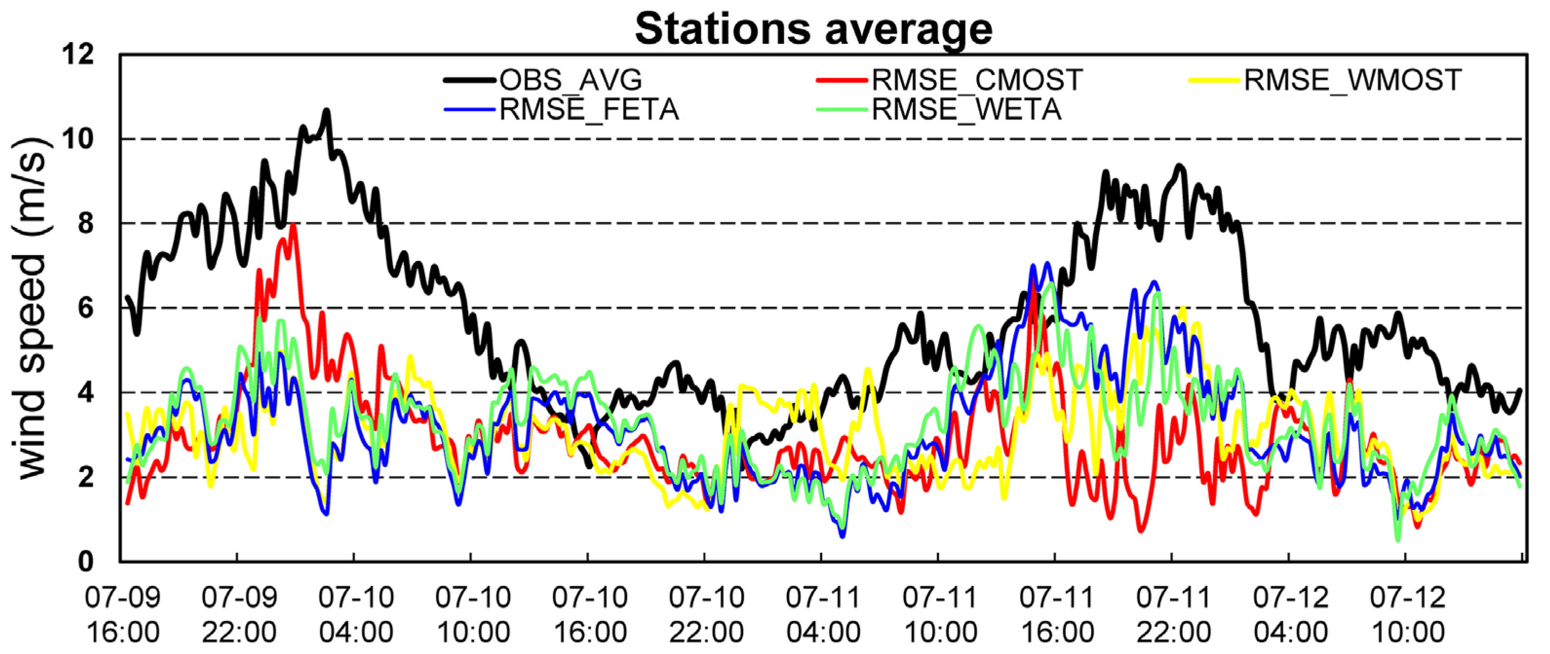
3.2. Differential Forecasting Performance on Wind Speed Fluctuation Characteristics
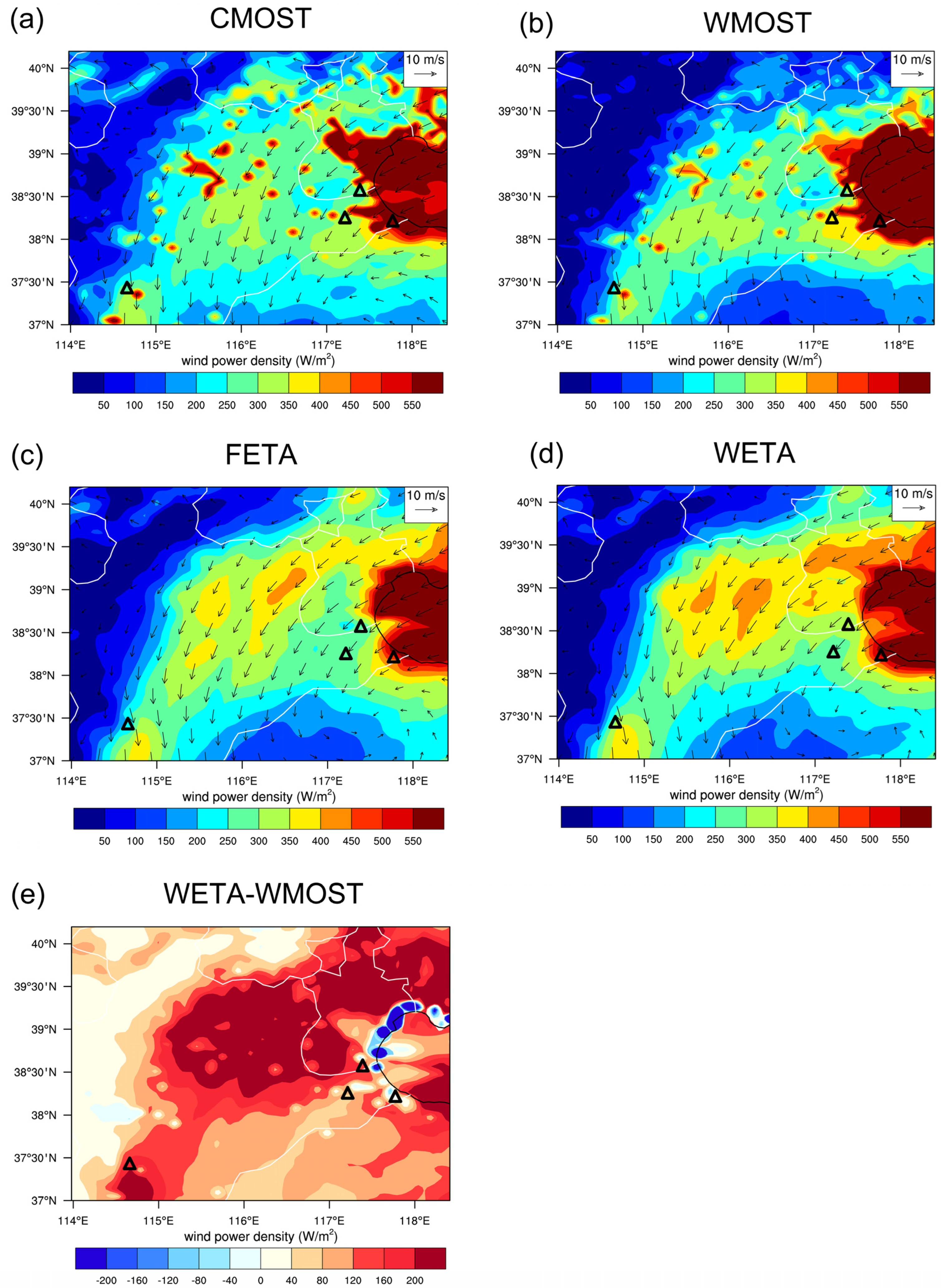
3.3. Spatial Variability in Wind Power Density Distribution
3.4. Analysis of the Influence of the PBL on Hub-Height Wind Speed Forecasts
4. Conclusions
Author Contributions
Funding
Institutional Review Board Statement
Informed Consent Statement
Data Availability Statement
Conflicts of Interest
References
- GWEC. G.W.E.C. Global Wind Report 2022; GWEC: Singapore, 2022. [Google Scholar]
- Porté-Agel, F.; Bastankhah, M.; Shamsoddin, S. Wind-turbine and wind-farm flows: A review. Bound. Layer Meteorol. 2020, 174, 1–59. [Google Scholar] [CrossRef]
- Baidya Roy, S.; Pacala, S.W.; Walko, R. Can large wind farms affect local meteorology? J. Geophys. Res. Atmos. 2004, 109, D19101. [Google Scholar] [CrossRef]
- Mo, J.; Huang, T.; Zhang, X.; Zhao, Y.; Liu, X.; Li, J.; Gao, H.; Ma, J. Spatiotemporal distribution of nitrogen dioxide within and around a large-scale wind farm—A numerical case study. Atmos. Chem. Phys. 2017, 17, 14239–14252. [Google Scholar] [CrossRef]
- Veers, P.; Dykes, K.; Lantz, E.; Barth, S.; Bottasso, C.L.; Carlson, O.; Clifton, A.; Green, J.; Green, P.; Holttinen, H. Grand challenges in the science of wind energy. Science 2019, 366, eaau2027. [Google Scholar] [CrossRef]
- Lundquist, J.K.; DuVivier, K.K.; Kaffine, D.; Tomaszewski, J.M. Costs and consequences of wind turbine wake effects arising from uncoordinated wind energy development. Nat. Energy 2019, 4, 26–34. [Google Scholar] [CrossRef]
- Al-Yahyai, S.; Charabi, Y.; Gastli, A. Review of the use of Numerical Weather Prediction (NWP) Models for wind energy assessment. Renew. Sustain. Energy Rev. 2010, 14, 3192–3198. [Google Scholar] [CrossRef]
- Olson, J.B.; Kenyon, J.S.; Djalalova, I.; Bianco, L.; Turner, D.D.; Pichugina, Y.; Choukulkar, A.; Toy, M.D.; Brown, J.M.; Angevine, W.M.; et al. Improving Wind Energy Forecasting through Numerical Weather Prediction Model Development. Bull. Am. Meteorol. Soc. 2019, 100, 2201–2220. [Google Scholar] [CrossRef]
- Chen, N.; Qian, Z.; Nabney, I.T.; Meng, X. Wind Power Forecasts Using Gaussian Processes and Numerical Weather Prediction. IEEE Trans. Power Syst. 2014, 29, 656–665. [Google Scholar] [CrossRef]
- Crippa, P.; Alifa, M.; Bolster, D.; Genton, M.G.; Castruccio, S. A temporal model for vertical extrapolation of wind speed and wind energy assessment. Appl. Energy 2021, 301, 117378. [Google Scholar] [CrossRef]
- Liu, B.; Ma, X.; Guo, J.; Li, H.; Jin, S.; Ma, Y.; Gong, W. Estimating hub-height wind speed based on a machine learning algorithm: Implications for wind energy assessment. Atmos. Chem. Phys. 2023, 23, 3181–3193. [Google Scholar] [CrossRef]
- García-Santiago, O.; Hahmann, A.N.; Badger, J.; Peña, A. Evaluation of wind farm parameterizations in the WRF model under different atmospheric stability conditions with high-resolution wake simulations. Wind Energ. Sci. 2024, 9, 963–979. [Google Scholar] [CrossRef]
- Liu, F.; Sun, F.; Liu, W.; Wang, T.; Wang, H.; Wang, X.; Lim, W.H. On wind speed pattern and energy potential in China. Appl. Energy 2019, 236, 867–876. [Google Scholar] [CrossRef]
- Li, M.; Shen, Y.; Yao, J.; Ye, D.; Fan, J.; Simmonds, I. An assessment of observed wind speed and wind power density over China for 1980–2021. Wind Energy 2022, 25, 2052–2070. [Google Scholar] [CrossRef]
- Bossavy, A.; Girard, R.; Kariniotakis, G. Forecasting ramps of wind power production with numerical weather prediction ensembles. Wind Energy 2013, 16, 51–63. [Google Scholar] [CrossRef]
- Zhou, B.; Duan, H.; Wu, Q.; Wang, H.; Or, S.W.; Chan, K.W.; Meng, Y. Short-term prediction of wind power and its ramp events based on semi-supervised generative adversarial network. Int. J. Electr. Power Energy Syst. 2021, 125, 106411. [Google Scholar] [CrossRef]
- Dyer, A.J.; Hicks, B.B. Flux-gradient relationships in the constant flux layer. Q. J. R. Meteorol. Soc. 1970, 96, 715–721. [Google Scholar] [CrossRef]
- Stull, R.B. An Introduction to Boundary Layer Meteorology; Springer Science & Business Media: Berlin/Heidelberg, Germany, 1988; Volume 13. [Google Scholar]
- Bahamonde, M.I.; Litrán, S.P. Study of the energy production of a wind turbine in the open sea considering the continuous variations of the atmospheric stability and the sea surface roughness. Renew. Energy 2019, 135, 163–175. [Google Scholar] [CrossRef]
- Barthelmie, R.J. Evaluating the impact of wind induced roughness change and tidal range on extrapolation of offshore vertical wind speed profiles. Wind Energy 2001, 4, 99–105. [Google Scholar] [CrossRef]
- Barthelmie, R.J.; Palutikof, J.P.; Davies, T.D. Estimation of sector roughness lengths and the effect on prediction of the vertical wind speed profile. Bound. Layer Meteorol. 1993, 66, 19–47. [Google Scholar] [CrossRef]
- Fischereit, J.; Brown, R.; Larsén, X.G.; Badger, J.; Hawkes, G. Review of Mesoscale Wind-Farm Parametrizations and Their Applications. Bound. Layer Meteorol. 2022, 182, 175–224. [Google Scholar] [CrossRef]
- Fitch, A.C.; Olson, J.B.; Lundquist, J.K.; Dudhia, J.; Gupta, A.K.; Michalakes, J.; Barstad, I. Local and Mesoscale Impacts of Wind Farms as Parameterized in a Mesoscale NWP Model. Mon. Weather Rev. 2012, 140, 3017–3038. [Google Scholar] [CrossRef]
- Wu, C.; Luo, K.; Wang, Q.; Fan, J. A refined wind farm parameterization for the weather research and forecasting model. Appl. Energy 2022, 306, 118082. [Google Scholar] [CrossRef]
- Archer, C.L.; Wu, S.; Ma, Y.; Jiménez, P.A. Two corrections for turbulent kinetic energy generated by wind farms in the WRF model. Mon. Weather Rev. 2020, 148, 4823–4835. [Google Scholar] [CrossRef]
- Peña, A.; Mirocha, J.D.; van der Laan, M.P. Evaluation of the Fitch Wind-Farm Wake Parameterization with Large-Eddy Simulations of Wakes Using the Weather Research and Forecasting Model. Mon. Weather Rev. 2022, 150, 3051–3064. [Google Scholar] [CrossRef]
- Lee, J.C.Y.; Lundquist, J.K. Evaluation of the wind farm parameterization in the Weather Research and Forecasting model (version 3.8.1) with meteorological and turbine power data. Geosci. Model Dev. 2017, 10, 4229–4244. [Google Scholar] [CrossRef]
- Mirocha, J.D.; Kosovic, B.; Aitken, M.L.; Lundquist, J.K. Implementation of a generalized actuator disk wind turbine model into the weather research and forecasting model for large-eddy simulation applications. J. Renew. Sustain. Energy 2014, 6, 013104. [Google Scholar] [CrossRef]
- Larsén, X.G.; Fischereit, J. A case study of wind farm effects using two wake parameterizations in the Weather Research and Forecasting (WRF) model (V3.7.1) in the presence of low-level jets. Geosci. Model Dev. 2021, 14, 3141–3158. [Google Scholar] [CrossRef]
- Jacobson, M.Z. Review of solutions to global warming, air pollution, and energy security. Energy Environ. Sci. 2009, 2, 148–173. [Google Scholar] [CrossRef]
- Waite, M.; Cohen, E.; Torbey, H.; Piccirilli, M.; Tian, Y.; Modi, V. Global trends in urban electricity demands for cooling and heating. Energy 2017, 127, 786–802. [Google Scholar] [CrossRef]
- Monin, A.S.; Obukhov, A.M. Basic laws of turbulent mixing in the surface layer of the atmosphere. Contrib. Geophys. Inst. Acad. Sci. USSR 1954, 151, e187. [Google Scholar]
- Jiménez, P.A.; Dudhia, J.; González-Rouco, J.F.; Navarro, J.; Montávez, J.P.; García-Bustamante, E. A Revised Scheme for the WRF Surface Layer Formulation. Mon. Weather Rev. 2012, 140, 898–918. [Google Scholar] [CrossRef]
- Businger, J.A.; Wyngaard, J.C.; Izumi, Y.; Bradley, E.F. Flux-profile relationships in the atmospheric surface layer. J. Atmos. Sci. 1971, 28, 181–189. [Google Scholar] [CrossRef]
- Fitch, A.C. Climate impacts of large-scale wind farms as parameterized in a global climate model. J. Clim. 2015, 28, 6160–6180. [Google Scholar] [CrossRef]
- Fitch, A.C.; Lundquist, J.K.; Olson, J.B. Mesoscale influences of wind farms throughout a diurnal cycle. Mon. Weather Rev. 2013, 141, 2173–2198. [Google Scholar] [CrossRef]
- Nakanishi, M.; Niino, H. An Improved Mellor–Yamada Level-3 Model: Its Numerical Stability and Application to a Regional Prediction of Advection Fog. Bound. Layer Meteorol. 2006, 119, 397–407. [Google Scholar] [CrossRef]
- Roberts, C.D.; Senan, R.; Molteni, F.; Boussetta, S.; Mayer, M.; Keeley, S.P.E. Climate model configurations of the ECMWF Integrated Forecasting System (ECMWF-IFS cycle 43r1) for HighResMIP. Geosci. Model Dev. 2018, 11, 3681–3712. [Google Scholar] [CrossRef]
- Thompson, G.; Field, P.R.; Rasmussen, R.M.; Hall, W.D. Explicit forecasts of winter precipitation using an improved bulk microphysics scheme. Part II: Implementation of a new snow parameterization. Mon. Weather Rev. 2008, 136, 5095–5115. [Google Scholar] [CrossRef]
- Zhang, C.; Wang, Y.; Hamilton, K. Improved representation of boundary layer clouds over the southeast Pacific in ARW-WRF using a modified Tiedtke cumulus parameterization scheme. Mon. Weather Rev. 2011, 139, 3489–3513. [Google Scholar] [CrossRef]
- Iacono, M.J.; Delamere, J.S.; Mlawer, E.J.; Shephard, M.W.; Clough, S.A.; Collins, W.D. Radiative forcing by long-lived greenhouse gases: Calculations with the AER radiative transfer models. J. Geophys. Res. Atmos. 2008, 113, D13103. [Google Scholar] [CrossRef]
- Tewari, M.; Wang, W.; Dudhia, J.; LeMone, M.A.; Mitchell, K.; Ek, M.; Gayno, G.; Wegiel, J.; Cuenca, R. Implementation and Verification of the United NOAH Land Surface Model in the WRF Model. 2016, pp. 11–15. Available online: https://www.researchgate.net/publication/286272692_Implementation_and_verification_of_the_united_NOAH_land_surface_model_in_the_WRF_model (accessed on 1 September 2024).
- North China Energy Regulatory Bureau of National Energy Administration. Detailed Implementation Rules for Auxiliary Service Management and Detailed Implementation Rules for Grid-connected Operation Management of Grid-Connected Power Plants in North China (in Chinese). Available online: https://hbj.nea.gov.cn/xxgk/fdzdgknr/hbjgfl/gfxwj/202311/t20231105_194947.html (accessed on 1 September 2024).
- South China Energy Regulatory Bureau of National Energy Administration. Detailed Implementation Rules for Auxiliary Service Management and Detailed Implementation Rules for Grid-Connected Operation Management of Grid-connected Power Plants in South China (in Chinese). Available online: https://nfj.nea.gov.cn/hdhy/zlxz/202402/t20240208_244591.html (accessed on 1 September 2024).
- Skamarock, W.C.; Klemp, J.B.; Dudhia, J.; Gill, D.O.; Liu, Z.; Berner, J.; Wang, W.; Powers, J.G.; Duda, M.G.; Barker, D.M. A description of the advanced research WRF version 4. NCAR Tech. Note Ncar/Tn-556+ Str 2019, 145. [Google Scholar]
- Smith, M.W. Roughness in the Earth Sciences. Earth Sci. Rev. 2014, 136, 202–225. [Google Scholar] [CrossRef]
- Garratt, J.R. The atmospheric boundary layer. Earth Sci. Rev. 1994, 37, 89–134. [Google Scholar] [CrossRef]
- Mihailović, D.T.; Lalić, B.; Rajković, B.; Arsenić, I. A Roughness Sublayer Wind Profile Above A Non-Uniform Surface. Bound. Layer Meteorol. 1999, 93, 425–451. [Google Scholar] [CrossRef]
- Emeis, S. A simple analytical wind park model considering atmospheric stability. Wind Energy 2010, 13, 459–469. [Google Scholar] [CrossRef]


| Parameterization Scheme | Option |
|---|---|
| Microphysics Parameterization | Thompson [39] |
| Convection Parameterization | New Tiedtke [40] |
| Long/Shortwave Radiation | RRTMG [41] |
| Near-Surface | Revised MM5 [33] |
| Land Surface | Noah [42] |
| Scenario | Model | WFP | Hub-Heights Wind |
|---|---|---|---|
| CMOST | CMA_WSP | / | ST based on 10 m |
| WMOST | WRF | OFF | ST based on 10 m |
| FETA | WRF_FITCH | ON | Interpolation from eta levels |
| WETA | WRF | OFF | Interpolation from eta levels |
| INDEX | STATION | CMOST | WMOST | FETA | WETA |
|---|---|---|---|---|---|
| RMSE | ZLD | 2.56 | 2.03 | 1.89 | 2.64 |
| YCZ | 2.75 | 3.56 | 3.68 | 3.26 | |
| HX | 4.65 | 4.16 | 4.66 | 4.68 | |
| YH | 3.31 | 4.19 | 3.71 | 3.43 | |
| R | ZLD | 0.75 | 0.71 | 0.81 | 0.82 |
| YCZ | 0.54 | 0.11 | 0.15 | 0.27 | |
| HX | 0.65 | 0.53 | 0.60 | 0.66 | |
| YH | 0.46 | 0.12 | 0.28 | 0.33 | |
| AR | ZLD | 74% | 80% | 81% | 74% |
| YCZ | 73% | 69% | 67% | 70% | |
| HX | 53% | 58% | 54% | 53% | |
| YH | 73% | 67% | 70% | 72% | |
| QR | ZLD | 80% | 69% | 90% | 73% |
| YCZ | 74% | 54% | 65% | 66% | |
| HX | 31% | 36% | 30% | 30% | |
| YH | 73% | 60% | 72% | 77% |
| INDEX | STATION | OBS | CMOST | WMOST | FETA | WETA |
|---|---|---|---|---|---|---|
| MIN | AVG | 2.24 | 3.66 | 3.13 | 3.64 | 4.02 |
| ZLD | 0.25 | 0.67 | 0.67 | 0.51 | 0.90 | |
| YCZ | 0.69 | 2.33 | 0.30 | 0.29 | 2.19 | |
| HX | 0.47 | 1.96 | 2.72 | 3.94 | 3.95 | |
| YH | 3.22 | 0.76 | 1.40 | 0.90 | 0.50 | |
| MIN BIAS RATIO | AVG | / | 64% | 40% | 63% | 80% |
| ZLD | / | 168% | 169% | 104% | 260% | |
| YCZ | / | 238% | −57% | −58% | 217% | |
| HX | / | 317% | 479% | 738% | 740% | |
| YH | / | −76% | −57% | −72% | −84% | |
| MAX | AVG | 10.65 | 14.97 | 11.29 | 11.65 | 12.26 |
| ZLD | 11.14 | 13.87 | 10.43 | 14.07 | 15.00 | |
| YCZ | 12.52 | 17.92 | 13.82 | 15.07 | 14.56 | |
| HX | 11.65 | 18.09 | 13.56 | 15.28 | 13.98 | |
| YH | 15.88 | 14.74 | 13.02 | 16.92 | 14.17 | |
| MAX BIAS RATIO | AVG | / | 41% | 6% | 9% | 15% |
| ZLD | / | 25% | −6% | 26% | 35% | |
| YCZ | / | 43% | 10% | 20% | 16% | |
| HX | / | 55% | 16% | 31% | 20% | |
| YH | / | −7% | −18% | 7% | −11% |
Disclaimer/Publisher’s Note: The statements, opinions and data contained in all publications are solely those of the individual author(s) and contributor(s) and not of MDPI and/or the editor(s). MDPI and/or the editor(s) disclaim responsibility for any injury to people or property resulting from any ideas, methods, instructions or products referred to in the content. |
© 2024 by the authors. Licensee MDPI, Basel, Switzerland. This article is an open access article distributed under the terms and conditions of the Creative Commons Attribution (CC BY) license (https://creativecommons.org/licenses/by/4.0/).
Share and Cite
Mo, J.; Shen, Y.; Yuan, B.; Li, M.; Ding, C.; Jia, B.; Ye, D.; Wang, D. Assessment of Numerical Forecasts for Hub-Height Wind Resource Parameters during an Episode of Significant Wind Speed Fluctuations. Atmosphere 2024, 15, 1112. https://doi.org/10.3390/atmos15091112
Mo J, Shen Y, Yuan B, Li M, Ding C, Jia B, Ye D, Wang D. Assessment of Numerical Forecasts for Hub-Height Wind Resource Parameters during an Episode of Significant Wind Speed Fluctuations. Atmosphere. 2024; 15(9):1112. https://doi.org/10.3390/atmos15091112
Chicago/Turabian StyleMo, Jingyue, Yanbo Shen, Bin Yuan, Muyuan Li, Chenchen Ding, Beixi Jia, Dong Ye, and Dan Wang. 2024. "Assessment of Numerical Forecasts for Hub-Height Wind Resource Parameters during an Episode of Significant Wind Speed Fluctuations" Atmosphere 15, no. 9: 1112. https://doi.org/10.3390/atmos15091112
APA StyleMo, J., Shen, Y., Yuan, B., Li, M., Ding, C., Jia, B., Ye, D., & Wang, D. (2024). Assessment of Numerical Forecasts for Hub-Height Wind Resource Parameters during an Episode of Significant Wind Speed Fluctuations. Atmosphere, 15(9), 1112. https://doi.org/10.3390/atmos15091112