Monthly Characteristics and Source–Receptor Relationships of Anthropogenic Total Nitrate in Northeast Asia

Abstract

The complex nonlinear characteristics of atmospheric chemistry necessitate the development of new methods for calculating source–receptor (S–R) relationships for secondary air pollutants. In this study, the monthly characteristics and S–R relationships of anthropogenic total nitrate (i.e., the sum of N from nitric acid, inorganic nitrate, and peroxyacetyl nitrate) in Northeast Asia were simulated and analyzed. The Community Multiscale Air Quality (CMAQ), Fifth-Generation NCAR/Penn State Mesoscale (MM5), and Sparse Matrix Operator Kernel Emissions (SMOKE) models were employed for air quality modeling, meteorological fields, and emissions processing, respectively. The study area encompassed Republic of Korea, Japan, and most of China. Five source/receptor regions were defined to derive the S–R relationships: three in China, one in Republic of Korea, and one in Japan. To produce data for the calculation of the S–R relationship, several experiments were conducted with a 20% reduction in NO_x emission sources. As a result of the S–R relationships, China was rarely impacted by the other two countries. The total depositions in other countries were significantly dominated by China (i.e., 43.5% and 40.7% in Republic of Korea and Japan, respectively, and up to 82.3% in December for Republic of Korea).

1. Introduction

The significance of long-range transboundary air pollutants (LTPs) in addressing air pollution has been increasingly emphasized in recent years. Air pollutants can travel long distances, ranging from hundreds to thousands of kilometers. Consequently, the source region can affect the air quality in the receptor region. Pollutants emitted from the source region can be transported over long distances by wind, meteorological conditions, and atmospheric chemical reactions, impacting regions far beyond their origin [1]. For example, industrial emissions from China often travel through air currents to Republic of Korea and Japan, exacerbating air pollution in those regions [2]. This issue is particularly prevalent in Northeast Asia, where the proximity of industrialized nations necessitates international cooperation to effectively manage air quality. Therefore, identifying source–receptor relationships is crucial for effectively addressing air pollution issues and plays an essential role in establishing effective air pollution mitigation policies. Especially, policymakers can leverage these relationships to coordinate with neighboring countries, ensuring that air pollution control measures are not confined to national borders but are implemented across the region. It can also improve international cooperation to address transboundary pollution problems. The persistent and rapid economic growth, high population density, and high energy consumption in Northeast Asia, encompassing Republic of Korea, China, and Japan, have resulted in various environmental issues. In regions characterized by close interconnections among multiple countries, a clear understanding of the relationships between the sources and receptors in each country is essential. The international dynamics in Northeast Asia underscore the need to address regional air pollution issues on a transnational scale, highlighting the importance of sharing scientific data and aligning national interests.

The long-range transport of air pollutants in Northeast Asia is a highly pertinent contemporary concern. China is responsible for large-scale emissions of sulfur dioxide (SO₂) and nitrogen oxides (NO_x) in Northeast Asia [3,4]. The impacts of the long-range transport of pollutant emissions from the industrial centers of eastern China and uplifted dust particles from the relatively dry regions further inland are severe [5,6]. Nitrogen dioxide (NO₂) concentrations in industrial areas of China have increased substantially in recent years, with an annual growth rate reaching at approximately 50% between 1996 and 2004 [7]. China’s rapid industrialization and urbanization have led to increased concentrations of secondary air pollutants, which can travel to Republic of Korea and Japan, significantly affecting air quality in those countries. This suggests that emissions from China can undermine air quality improvement efforts in neighboring countries, necessitating collaborative responses. This study was conducted as a part of the LTP project, which is a joint research project on LTPs in Northeast Asia. The National Institute of Environmental Research (NIER) of Korea initiated this collaborative project to study and analyze LTPs in Northeast Asia, specifically in China, Japan, and Republic of Korea. The source–receptor relationship between the three countries in terms of total nitrate is an important aspect of the LTP project [8]. Nitrate, which forms as a secondary pollutant through complex atmospheric reactions, can accumulate across multiple countries due to long-range transport [9]. These substances often precipitate with rain, leading to soil and water pollution, significantly impacting ecosystems. Therefore, accurately determining the source–receptor relationships for total nitrate is crucial for improving air quality and developing environmental protection policies. Furthermore, calculating the source–receptor relationships for certain pollutants, particularly secondary air pollutants, necessitates establishing more diverse methodologies because of the complex nonlinear characteristics of atmospheric chemistry. Secondary pollutants such as nitrate are heavily influenced by precursor substances like ammonia (NH₃) and peroxyacetyl nitrate (PAN). NH₃ primarily originates from agricultural activities, fossil fuel combustion, and vehicular emissions, while PAN is formed from the reaction of volatile organic compounds (VOCs) and nitrogen oxides (NOx) under photochemical conditions [10]. Understanding the sources and transformations of these precursors is essential for accurately determining the source–receptor relationships for nitrate, as these interactions are crucial in the formation of secondary pollutants. To achieve this, three-dimensional atmospheric chemical models should be utilized. These models can simulate how pollutants move and transform in the atmosphere, providing a more accurate analysis of source–receptor relationships.

In this study, we aimed to gain insights into the monthly characteristics and source–receptor relationships of anthropogenic total nitrate in Northeast Asia. To achieve this, we performed numerical simulations using the Community Multiscale Air Quality (CMAQ) modeling system. The US Environmental Protection Agency (EPA) Models-3/CMAQ model was utilized to calculate the source–receptor relationships for total nitrate in Northeast Asia. The meteorological model used was the Fifth-Generation NCAR/Penn State Mesoscale Model (MM5), while the emission data were processed using the Sparse Matrix Operator Kernel Emissions (SMOKE) modeling system. Moreover, this study utilized the emission data from the Intercontinental Chemical Transport Experiment Phase B (INTEX-B) and Transport and Chemical Evolution over the Pacific (TRACE-P) for the East Asia region.

2. Materials and Methods

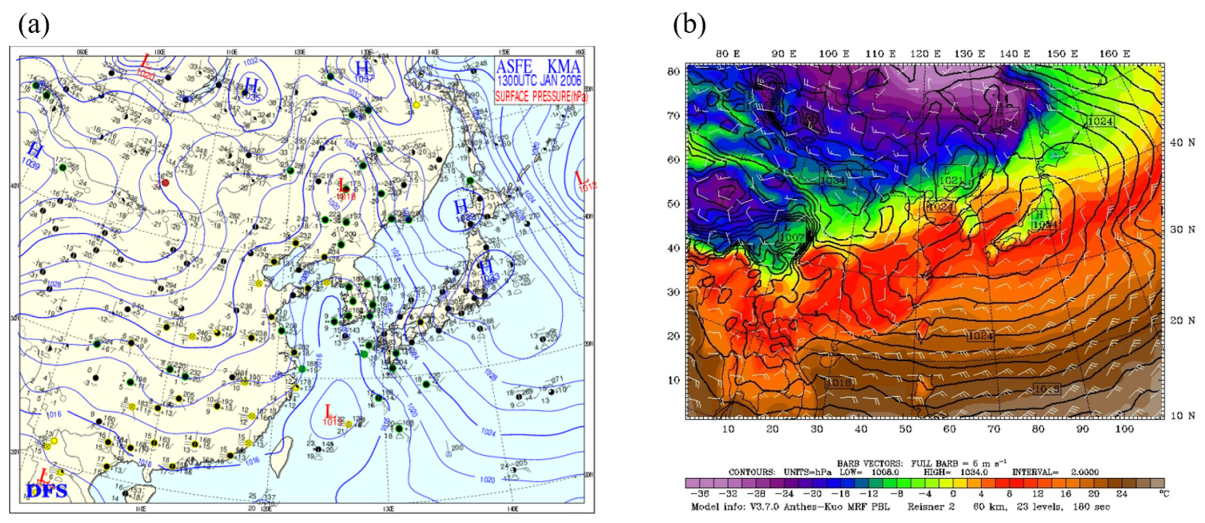
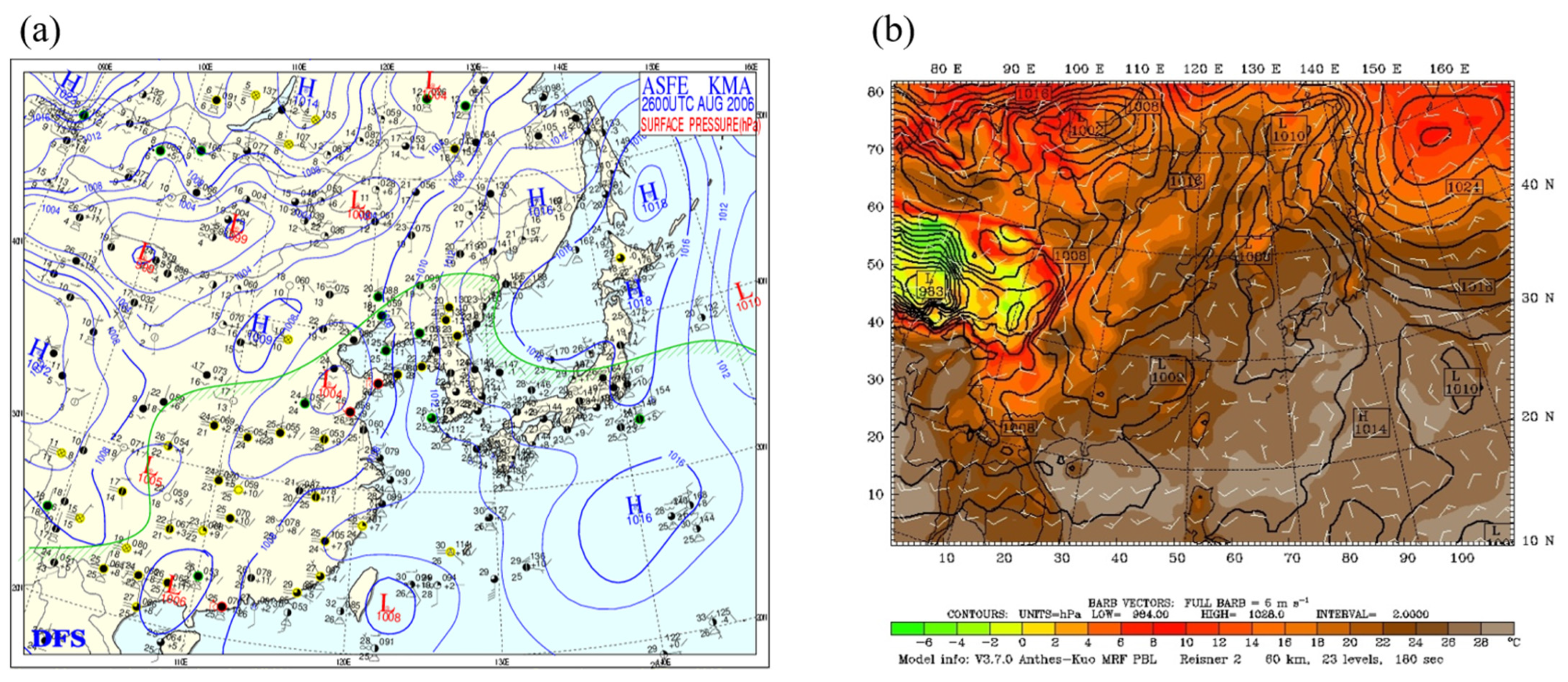
2.1. Meteorological Model

MM5v.3.7 [11] was used to produce and provide the meteorological fields for CMAQ (wind, temperature, water mixing ratio, precipitation, and surface variables). The National Center for Environmental Prediction (NCEP) FNL reanalysis data, with 1.0 × 1.0° resolution and 6-h time intervals, were used to establish initial and boundary conditions for meteorological fields. Four-dimensional data assimilation (FDDA) was employed to improve the model results. Domain 1 for the nesting process consisted of a 51 × 47 grid in the plane with a 180 km grid resolution. Domain 2 of the MM5 was larger than that of the CMAQ, with its center positioned at 37° N and 123° E. There were 109 × 82 grids in the plane with a 60 km grid resolution and 24 vertical sigma layers with varying thicknesses. The top height was set at 100 hPa. The sigma levels were 1.00, 0.99, 0.98, 0.96, 0.93, 0.89, 0.85, 0.80, 0.75, 0.70, 0.65, 0.60, 0.55, 0.50, 0.45, 0.40, 0.35, 0.30, 0.25, 0.20, 0.15, 0.10, 0.05, and 0.00.

Among the advantages, the MM5v3.7 model offers flexible domain configuration, allowing researchers to adjust the model to the specific geographic and meteorological characteristics of the region being studied [12]. This flexibility is a significant strength when dealing with diverse regional conditions. Additionally, the use of FDDA (Four-Dimensional Data Assimilation) provides an opportunity to enhance the accuracy of the modeling results by assimilating observational data. However, the model also has limitations. For instance, it may struggle to capture fine-scale meteorological patterns such as urban heat island effects or small-scale convective phenomena. The 60 km resolution may not be sufficient to fully represent these detailed phenomena [13]. Nevertheless, since this study focuses on Northeast Asia, including China, Republic of Korea, and Japan, the limitations related to capturing fine-scale meteorological patterns are relatively less critical. Furthermore, as with all meteorological models, there is inherent uncertainty in the model outputs, which can be influenced by the input data and the parameterized physical processes within the model. So, this study evaluated the meteorological model results as part of the results.

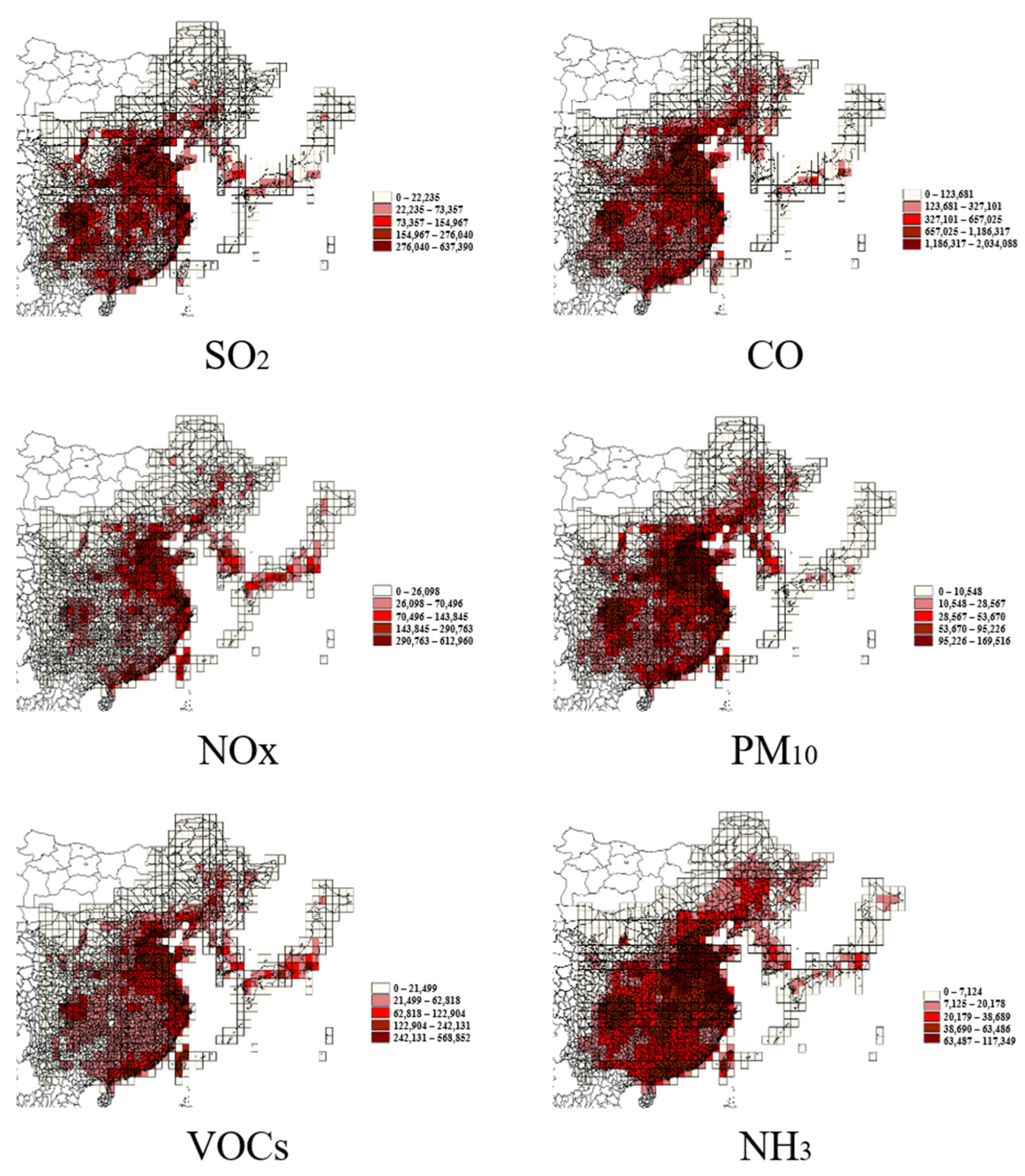
2.2. Emission Framework

Emission datasets for anthropogenic SO₂, CO, NO_x, PM₁₀, volatile organic compounds (VOCs), and NH₃ were prepared and supplied, as depicted in Figure 1. Emission datasets covered 20–50° N in latitude and 100–150° E in longitude, except for certain regions such as Mongolia and Southeast Asia. The SO₂, CO, NO_x, PM₁₀, and VOC emissions were based on the INTEX-B emission inventory [14], which was derived from the Center for Global and Regional Environmental Research (CGRER), University of Iowa. Gridded data from the 0.5 × 0.5° INTEX-B were converted into 1 × 1° gridded emission data. INTEX-B is an emission inventory developed as part of a project aimed at quantifying air pollution emissions and long-range transport in Asia. It is a highly comprehensive and geographically extensive inventory that includes emission data from various pollution sources across Northeast Asian countries such as Republic of Korea, China, and Japan.

NH₃ emissions were not included in INTEX-B. Therefore, we estimated the regional NH₃ emissions in our domain by projecting the TRACE-P emission inventory [15] using projection factors derived from the Regional Emission Inventory in Asia (REAS) [16]. PM_2.5 emissions were obtained from the INTEX-B emissions inventory, which was derived from the CGRER. Volcanic emissions derived by the LTP secretariat [8] were included with a release height of approximately 1500 m [17]. Natural emissions, such as biogenic VOCs, NO_x from the soil, and lightning, were not considered. The source sectors in INTEX-B and TRACE-P (for NH₃) were reorganized based on the Emission Database for Global Atmospheric Research (EDGAR) [18] and mapped with the US EPA’s source classification codes (SCCs). The emissions sources and source activities of INTEX-B and TRACE-P are shown in

Table 1. Emission source’s activities.

INTEX-B	Source Description
Power	Power generation
	Small power generation
Industry	Industry
	Charcoal production
	Industrial sector
	OTS(ALL)-Other transformation sector
	Oil production
	Gas production
	IRO: Iron & steel
	NFE: Non-ferro
	CHE: Chemicals
	Building materials
	PAP: Pulp & paper
	FOOD: Food (Beer & Wine)
	SOL: Solvent use/MISC.
	MIS: ind. MISCELLANEOUS
	MISC: Waste handling
Residential	RCO: Residential
	RCO sector (RES + COM + OTH)
	Waste incliner (non-energy)
Transportation	Road transport (ETH.)
	Road transport (INCL. EVA)
	TRANS. LAND NON-ROAD
TRACE-P	Source Description
Cattle, pigs	Domestic animal
O_animal	Wild Animals
PERTI	Synthetic Fertilizer (Fertilizer use)
BIOF	Industry and other trans & residential
Other	Crop
	Fossil fuel use (include other trans and road transport
	Human population
	Industrial process(chemicals)

.

Moreover, geographic information system (GIS) techniques were utilized to convert gridded emissions into admin-based emissions for preparing USEPA’s IDA format, which was the input format of emissions for SMOKE [19]. The modeling emissions inventory was generated using SMOKEv.3.5, incorporating the Statewide Air Pollution Research Center (SAPRC99) chemical mechanism. The gridded emissions of SO₂, CO, NO_x, PM₁₀, VOCs, and NH₃ are shown in Figure 1.

Monthly variations were taken into account when creating the emission dataset for the CMAQ model. The gridding profile, which was the input for SMOKE, was developed using the Multimedia Integrated Modeling System (MIMS) Spatial Allocator with GIS data, such as high-resolution administration boundary data, land cover, road networks, population (rural, urban, and total), forest, and cropland.

2.3. Air Quality Model

Three-dimensional Eulerian modeling over Northeast Asia was performed using the US EPA Models-3/CMAQ model [20]. CMAQ v.5.0.2 was employed in this study. In this modeling study, the SAPRC99, ISORROPIA, and Regional Acid Deposition Model (RADM) modules were selected for the gas-phase chemistry, aerosol module, and dry/wet deposition for gaseous and particulate species, respectively. The CMAQ model is particularly well-suited for the study of secondary pollutants such as nitrates and ozone because it can simulate a wide range of physical processes and photochemical reactions [21]. However, the model also has limitations. Like meteorological models, the performance of the CMAQ model is influenced by the quality of the input data [21]. This means that inaccuracies in the input data can lead to uncertainties in the model’s predictions, affecting the reliability of the results.

Hourly meteorological fields were prepared using MM5 v.3.7 with FDDA and subsequently provided to the CMAQ, as described above. The initial concentrations were assumed to be zero for all substances, except for O₃, where a concentration of 40 ppb was assumed at the initial time and inflow boundaries. However, the MM5 and CMAQ modeling periods commenced 5 d before the first day of each month to align the chemical species with their actual state in the atmosphere.

The study area encompassed the region of 100–150° E longitude and 20–50° N latitude. This area included the entirety of Republic of Korea, Japan, most of China, and parts of Mongolia, Russia, and Southeast Asia. The Lambert-Conformal projection was applied. The horizontal grid spacing was 60 × 60 km (the number of grids in the x- and y-directions were 90 and 60, respectively). The vertical conditions were the same as the meteorological conditions.

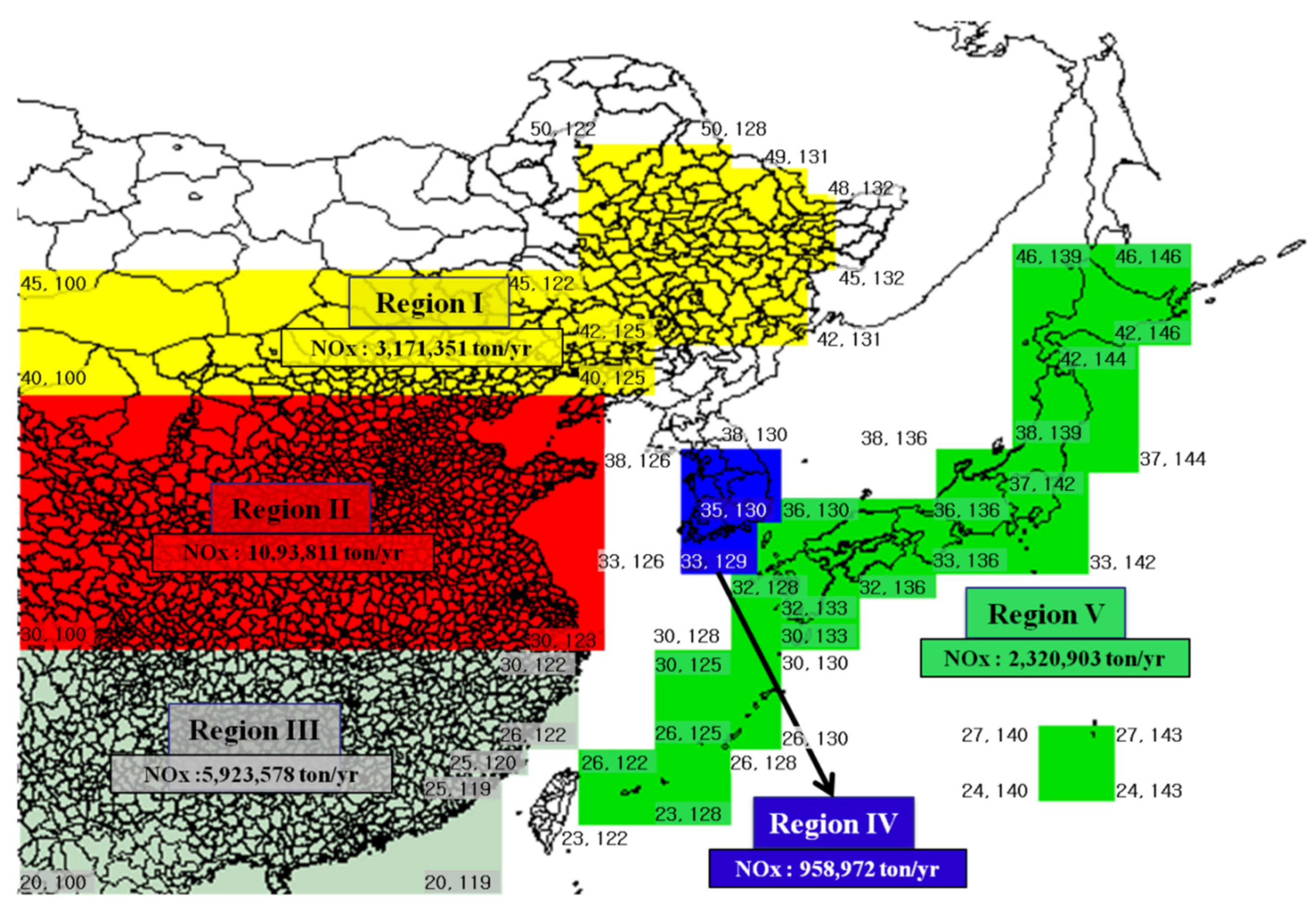
2.4. Source–Receptor Methodology

The source–receptor regions were identical to those in the Annual Report of the Working Group of the LTP project 2005 [22], except for Region 4. Five source/receptor regions were defined to derive the source–receptor (S–R) relationship: three in China (Region 1, northern China; Region 2, central China; and Region 3, southern China), one in Republic of Korea (Region 4), and one in Japan (Region 5). In this study, the northern boundary of Region 4 was expanded from 37° N to 38° N to include the Seoul Metropolitan Area and a portion of Gangwon Province in Republic of Korea, as depicted in Figure 2. The Brute-Force method was applied in this study for analyzing the source–receptor relationships. This method was similar to the EMEP Method 3 [23]. According to this method, the deposition resulting from emissions in a specific area is computed by taking the difference (multiplied by 10) between the model run with all emissions and the model run with a 10% emission reduction from that specific area. However, the 20% NO_x reduction case yielded the best results. Therefore, the reduction was adjusted to a 20% decrease.

The S–R relationship can be calculated using the following formulas:

$${\mathit{C}}_{\mathit{i}\mathit{j}}={\displaystyle \frac{{\mathit{D}}_{\mathit{i}\mathit{j}}}{{{\displaystyle \mathit{\sum }}}_{\mathit{i}=\mathbf{1}}^{\mathit{n}}{\mathit{D}}_{\mathit{i}\mathit{j}}}}\mathit{\times }\mathbf{100} \left(\mathbf{\%}\right),$$

(1)

$${\mathit{D}}_{\mathit{i}\mathit{j}}=\left(\mathit{D}\mathit{b}\mathit{a}\mathit{s}\mathit{e}-\mathit{D}\mathit{i}\right)÷\mathit{R}\mathit{D},$$

(2)

where C_ij is the contribution of the i-th emission source to the j-th receptor, while D_ij is the deposition amount at the j-th receptor caused by the i-th source. D_ij is obtained as the difference between the results of the base-case simulation (uncontrolled, all emission sources, D_base) and controlled-emission simulation (20% NO_x emission reduction from the ith source, D_i). RD is the percentage reduction (i.e., 20% in this study). n = 5 because the domain is divided into five source–receptor regions. The S–R relationships of ‘total nitrate’ were analyzed. We defined ‘total nitrate’ as the sum of nitrogen from nitric acid (HNO₃), inorganic nitrate (NO₃⁻), and peroxyacetyl nitrate (PAN). The CMAQ simulation findings define NO₃⁻ as the combined total of ANO3I and ANO3J.

To explain Equation (2) in more detail, the deposition, D_ij, represents the total nitrate deposition at the j-th receptor caused by the NOx emissions from the i-th source. This is calculated by comparing the deposition results from two simulations: the base case simulation, D_base, where all emissions are fully accounted for, and a controlled emission simulation, D_i, where NOx emissions from the i-th source are reduced by 20%. The difference between these two simulations provides the deposition due to 20% of the NOx emissions from the i-th source. Dividing this difference by 0.2 (the percentage reduction) allows us to estimate the total deposition at the j-th receptor caused by 100% of the NOx emissions from the i-th source.

3. Results and Discussion

3.1. Comparison of Predicted Meteorological Fields with Observations

The simulated sea-level pressure systems were compared with those from the observational data to verify their performance in four specific cases (00 UTC on 13 January, 19 April, 26 August, and 9 September 2006). Figure 3 displays the observational data of 00 UTC on 13 January, revealing a low-pressure system in the Manchuria region and a high-pressure system in Japan. The simulation results indicated a similar pattern. However, the pressure patterns in the south-central region of China exhibited certain differences between the observational data and simulation results.

In the observational data of 00 UTC on 19 April (Figure 4), a low-pressure system formed in the Manchuria region; however, these data were also slightly different from the simulation results. Observational data showing a low-pressure system in the western region of China corresponded with the results of the model.

At 00 UTC on 26 August, a low-pressure system developed over the Korean Peninsula and most regions of China, whereas a high-pressure system formed over Tokyo and Hokkaido in Japan in the observations, as depicted in Figure 5. The simulation results exhibited the same pattern. However, on the Korean Peninsula, a slight difference was observed between the observational data and simulation results. The simulated sea-level pressure systems were compared with those of the observational data at 00 UTC on 9 September, as shown in Figure 6. In the observational data, high-pressure systems formed in the Tokyo region and the northern region of China, while a low-pressure system formed in Osaka. The model simulation results mostly exhibited the same pattern.

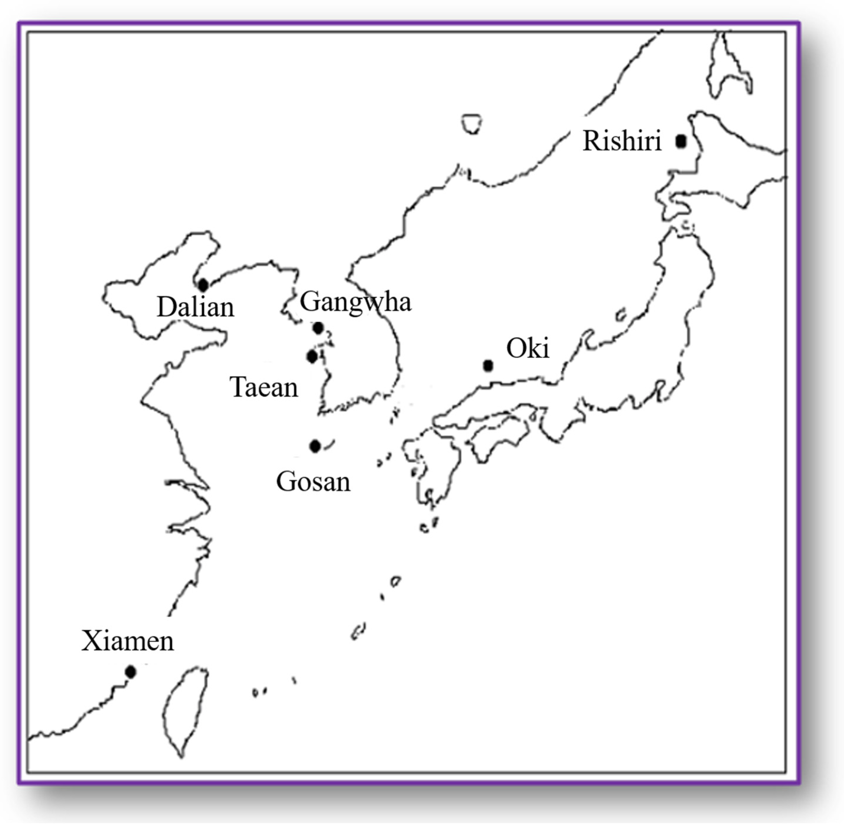
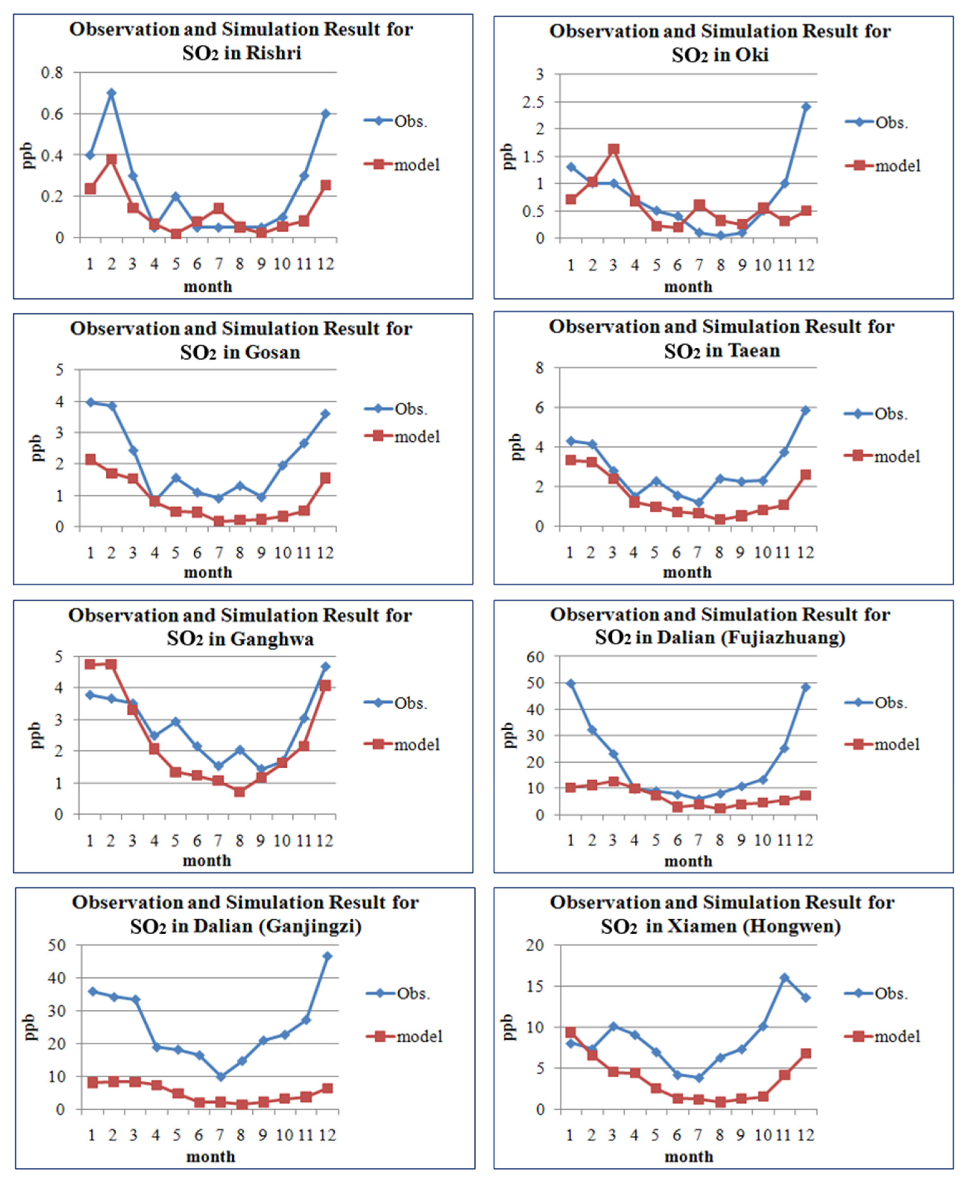
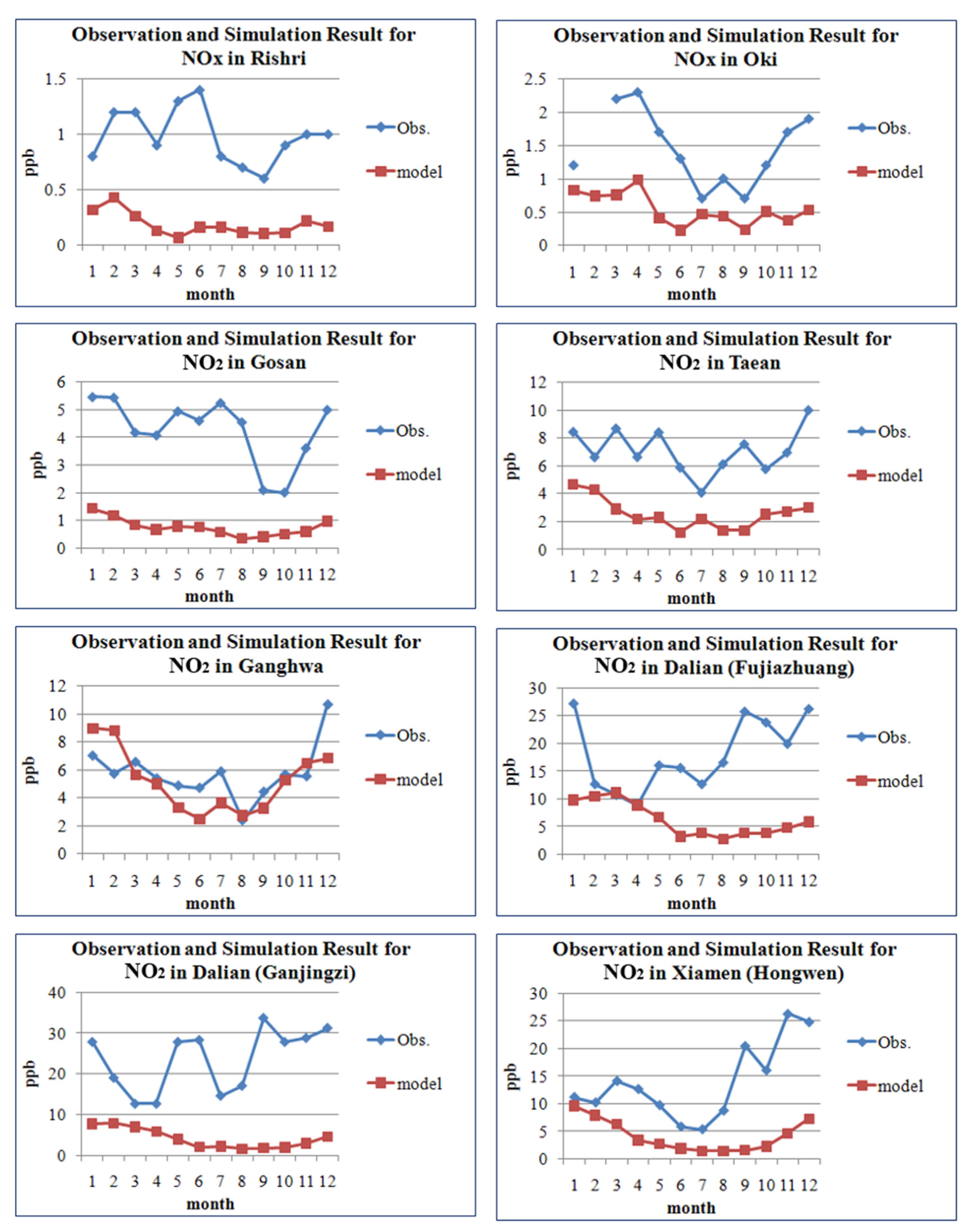
3.2. Comparison of Air Quality Modeling Results with Observations

Figure 7 shows the air pollution monitoring stations in the Northeast Asia region. In this study, monthly average data from 2006 were used to compare and analyze the air quality modeling results with the measured values for SO₂ and NO₂.

The modeling results for SO₂ were relatively consistent with the measured values at background monitoring stations in Japan, such as Rishiri and Oki, and at background monitoring stations in Republic of Korea, including Gosan, Taean, and Ganghwa. However, in China, particularly in the Dalian region at Fujiazhuang and Ganjingzi, the SO₂ concentrations were underestimated during winter. This underestimation is likely due to an increase in atmospheric SO₂ concentrations from local winter emissions not accounted for in the emission inventory. The results of this comparison are presented in Figure 8.

For NO₂, there were significant discrepancies between the modeling results and the measurements depending on the region. In Ganghwa, located near the metropolitan area of Republic of Korea, the monthly variation trends and concentration levels were relatively well simulated. However, in Dalian, Xiamen, and Gosan, the NO₂ concentrations were only about 20–35% of the measured values, and the monthly trends were not well captured. While the measured values showed significant monthly variations, the simulated NO₂ concentrations exhibited smaller fluctuations. The results of this comparison are presented in Figure 9.

Overall, the modeling results for SO₂ and NO₂ were generally lower than the measured values. One of the causes of the underestimation appears to be the absence of natural emissions, excluding volcanic emissions, in the emissions inventory used in this study. Additionally, the difference between the model results and the measured values may be because the measurement points were single locations, while the model grid size used for comparison was 60 × 60 km.

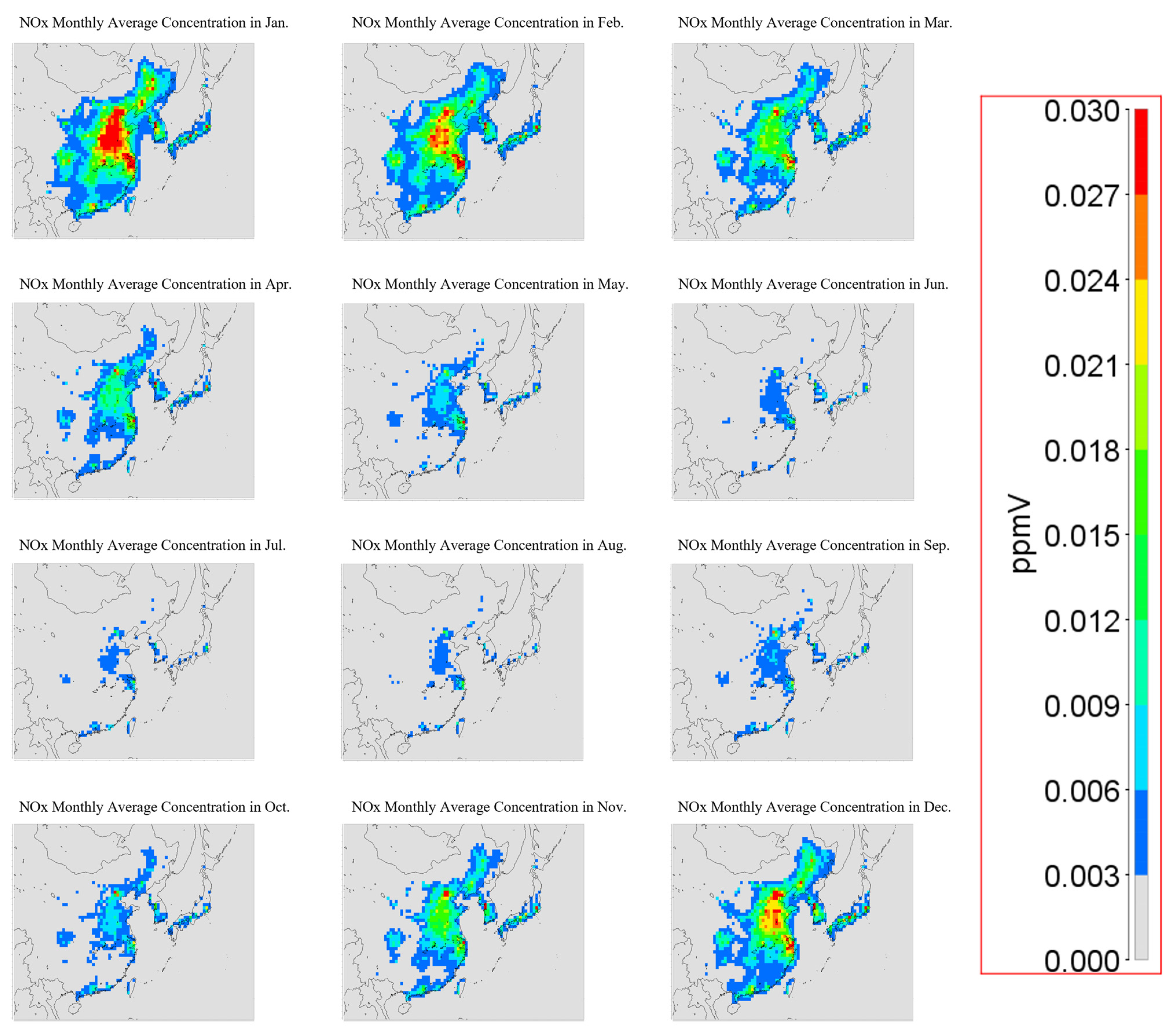
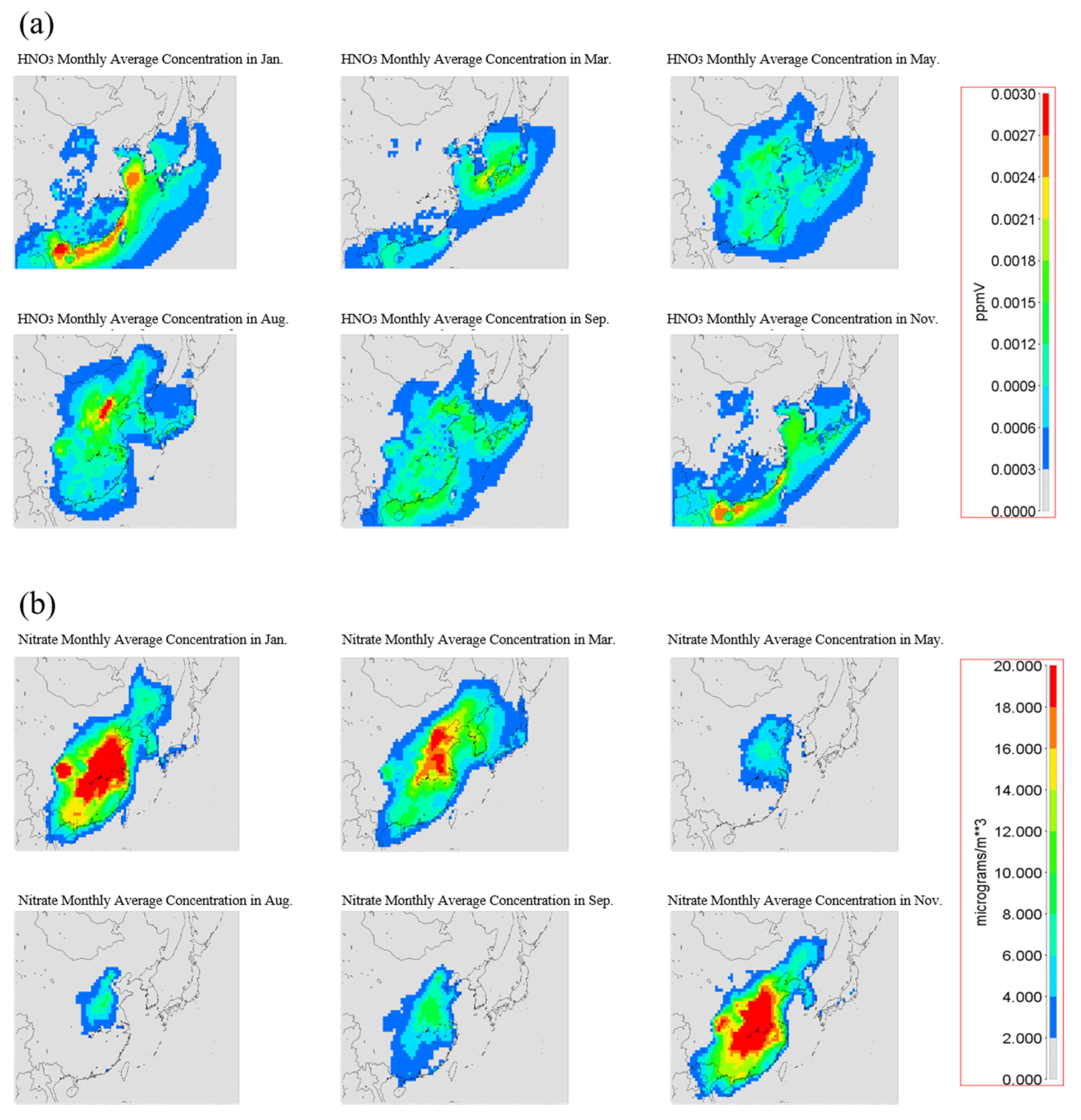
3.3. Spatial Distributions of Monthly Mean Concentrations

The spatial distributions of the primary gaseous species, such as SO₂, NO_x, and NO₂, nearly overlapped with those of their emissions. During the 12 months, relatively high NO_x concentrations occurred in winter, particularly in January. In contrast, low NO_x concentrations were observed in summer, as shown in Figure 10.

The spatial distributions of NO_x exhibited high concentrations in eastern China along the Yellow Sea, Republic of Korea, and southern Japan. These distributions overlapped with the industrial areas of China, the Seoul metropolitan area of Republic of Korea, and the Tokyo area of Japan [24,25,26]. This suggested that the seasonal variation of NO₂ was explained by regional emissions and photochemistry-related relatively short lifetimes (less than a day), as well as higher winter emissions.

In fine-mode particles, the major form of nitrate was the NH₄NO₃ crystallized salt. NH₄NO₃ salt formation or NH₄⁺-NO₃⁻ ion association occurred via the following equilibrium reaction [27,28]:

NH₃(g) + HNO₃(g) ↔ NH₄NO₃(s) and/or NH₄⁺ (aq) + NO₃⁻ (aq)

The equilibrium of this reaction is governed by thermodynamic relationships. When the temperature is low, the equilibrium shifts toward particulate NH₄NO₃ or NH₄⁺-NO₃⁻ formation. Conversely, when the temperature is high, it proceeds in the reverse direction. The ISORROPIA module in the Models-3/CMAQ model takes into account this heterogeneous process [29], where both forward and reverse reactions occur so rapidly that these processes can be treated thermodynamically [30].

Figure 11 illustrates the spatial distributions of nitric acid and nitrate for 6 months.

As previously mentioned, the nitric acid concentrations in the atmosphere were sensitive to temperature. In January, high distributions of nitric acid concentration occurred in the near ocean relative to inland because the temperature near the ocean was higher than inland. Higher nitric acid concentrations migrated towards the continent in August, and the spatial distribution of nitric acid exhibited high concentrations in Region 2 (central China). When the temperature over the continent begins to decrease, the relatively higher nitric acid distributions return to the near ocean, as in November.

The nitrate concentrations were primarily distributed in China, with considerable presences in Region 4 (Republic of Korea) and the south of Region 5 (Japan) in January and April. The highest nitrate concentrations occurred in eastern and western China during winter. In contrast to nitric acid concentrations, low nitrate concentrations were observed in August in China. Most of the nitrate concentrations observed in winter and spring in this region were of Chinese origin.

The NO_x and PAN concentration distributions exhibited similar trends to the nitrate concentration distribution, with concentrations gradually decreasing from winter to summer and increasing again in the fall. The concentration distribution of NO_x was scattered throughout the entire region (China, Republic of Korea, and Japan); however, the highest NO_x concentrations also occurred in China. In January, the spatial distribution of NO_x was the highest in the eastern part of Region 2 (central China). Conversely, the highest PAN concentration was observed in the western part of Region 2, and there was a high distribution of PAN concentrations in Region 3 (southern China) during winter. The spatial distributions of PAN in winter, spring, and fall were widespread across China, Republic of Korea, and Japan.

The O₃ concentration reached 53 ppb during August. However, the O₃ concentrations in China were the lowest in January and December. Interestingly, higher O₃ concentrations occurred above the oceans in April, especially between China and Republic of Korea.

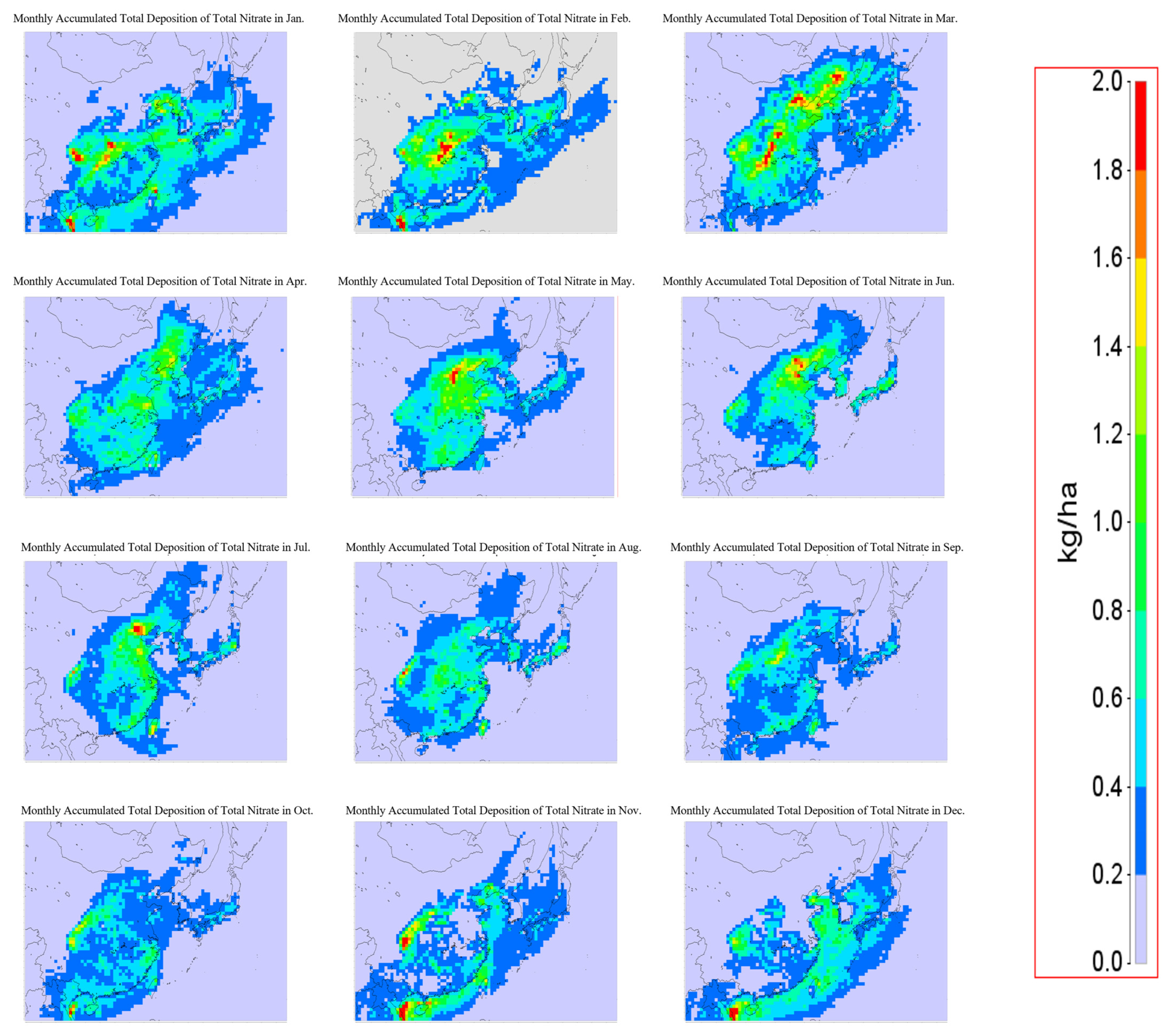
3.4. Characteristics of Total Nitrate Deposition

The monthly accumulated wet deposition of inorganic nitrate was more dominant than the dry deposition; therefore, the spatial distribution of the total deposition of inorganic nitrate was similar to that of the wet deposition. The dry deposition of inorganic nitrate exhibited high values in spring (except May) and winter on the Chinese continent. In addition, high values were observed in December along the east coast of China. We observed high values of inorganic nitrate dry deposition on land in eastern China in April, particularly along the coast. In contrast, low values of inorganic nitrate dry deposition occurred in Region 2 (central China) in August. The distribution of inorganic nitrate wet deposition was similar to that of NO_x emissions and precipitation. This was because wet N deposition was primarily a result of in-cloud scavenging (‘rainout’) and below-cloud scavenging (‘washout’) of atmospheric N constituents [31].

The total amount of deposited nitric acid was approximately 30% of the inorganic nitrate. In contrast, the monthly accumulated dry deposition of nitric acid was more dominant than wet deposition; therefore, the spatial distribution of the total deposition of nitric acid was the same as that for dry deposition. The spatial distribution of the monthly accumulated nitric acid total deposition varied each month, with a trend of higher nitric acid total deposition near the coast in January, shifting inland in August, and then returning to near the ocean in September. The wet-to-total deposition ratio of nitric acid was approximately 0.02. However, the wet depositions in August and September were considerably lower than those in January. Specifically, the nitric acid deposition in January was 377 times higher than that in September, which appeared mainly in the northeastern regions of our domain.

Among the target pollutants, the proportion of PAN to total nitrate was small. The amount of dry PAN deposition dominated the wet deposition; therefore, the spatial distribution of total PAN deposition was the same as that of dry deposition. Figure 12 displays the spatial distributions of the monthly accumulated total nitrate depositions.

The wet deposition of total nitrate had the highest contribution from the inorganic nitrate wet deposition; therefore, the spatial distribution of the total nitrate wet deposition was similar to that of the inorganic nitrate wet deposition. In contrast, nitric acid dry deposition contributed most significantly to the total nitrate dry deposition; therefore, the spatial distribution of the total nitrate dry deposition was similar to that of the nitric acid dry deposition. The distribution of the total deposition of total nitrate was similar to that of monthly wet deposition because of the dominant dry conditions.

For total deposition, elevated levels of total nitrate appeared in Region 2 in January, February, and March; however, in Region 1, elevated levels of total nitrate occurred in May, June, and July. In summer, the total nitrate dry deposition was distributed in most of the five spatial regions. However, the total nitrate wet deposition exhibited the opposite pattern.

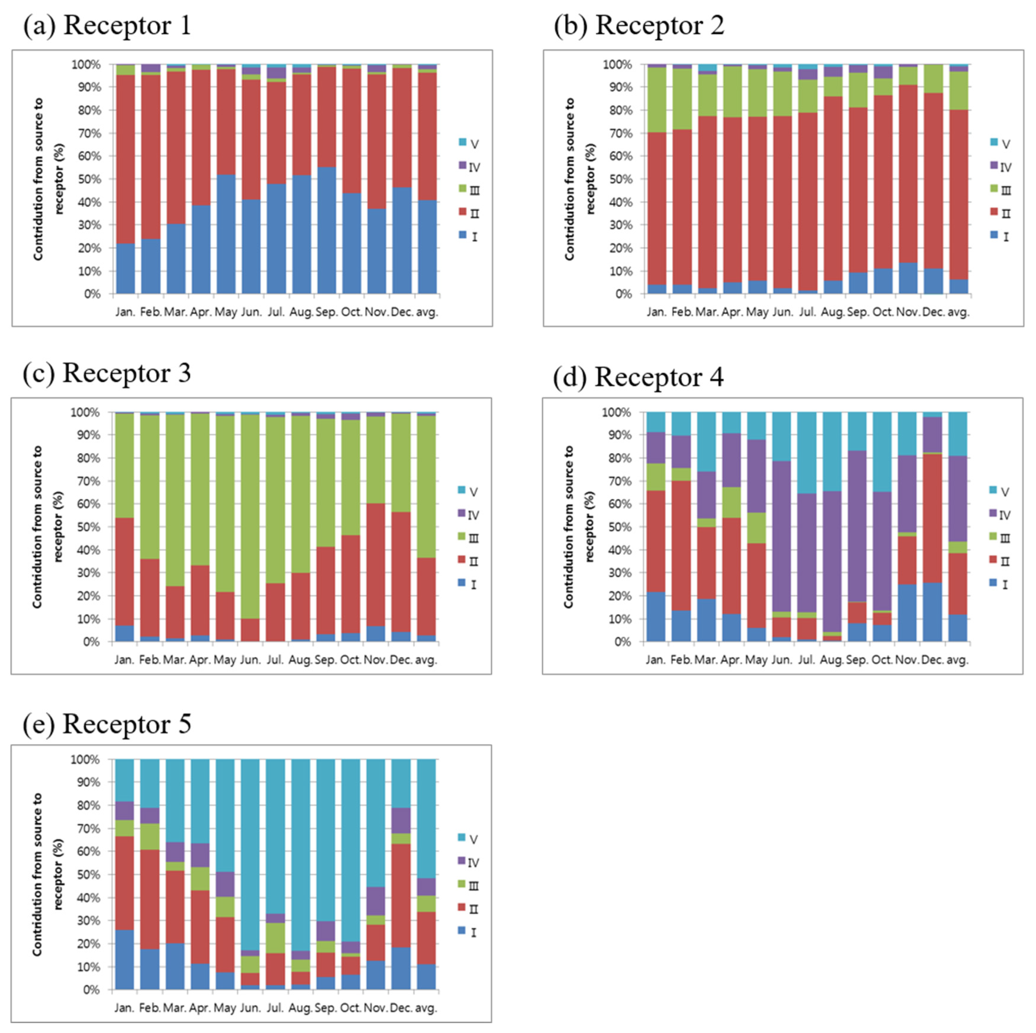
3.5. Source–Receptor Relationship of Total Nitrate in East Asia

The monthly and average source–receptor contributions for the total deposition of total nitrate are illustrated in Figure 13. The average self-contributions of the five regions were 40.8, 73.8, 61.8, 37.3, and 51.6%, respectively, and were the dominant contributions for all regions except Region 1.

China experienced minimal impact from the other two countries. The country-aggregate self-contributions of China for Regions 1, 2, and 3 were 97.8, 96.8, and 98.3%, respectively. The total depositions in other countries were also significantly dominated by China (43.5% and 40.7% in Regions 4 and 5, respectively, and up to 82.3% in December for Region 4). The contributions of Region 2 influenced all regions in most cases because they had the largest NO_x emissions and were geographically the closest. Lin et al. [32] observed that long-range transport from industrialized areas of China contributes to a significant percentage (>20%) of the anthropogenic reactive nitrogen depositions throughout East Asia.

For Region 4, the average contributions from long-range transport for Regions 1, 2, and 3 combined and Japan were 43.5% and 19.2%, respectively. Consequently, LRT was more dominant than self-contribution. The PM₁₀ contribution from China to the Seoul Metropolitan Area can reach as high as 80% in January [33,34]. In addition, our study showed that the maximum impact of China on Region 4 was 77.6%.

During July and August, Region 5 accounted for approximately 35% of the total nitrogen deposition in Region 4. This could be explained by long-range transport associated with seasonal wind patterns, specifically the influence of northwesterly winds from the Pacific on East Asia during summer. The contributions from Regions 4 and 5 to Regions 1 and 2 also exhibited a 1.7–2.9-fold increase for the same months.

Table 2. Comparison between this study and Lin et al. [32] estimating the source–receptor relationships for total nitrogen deposition (in percent).

	Receptors	China		Republic of Korea		Japan
Source		This Study	Lin (2008)	This Study	Lin (2008)	This Study	Lin (2008)
China		97.5	79.7	43.5	39.1	40.7	20.6
Korea		1.8	2.6	37.3	46.9	7.7	14.9
Japan		0.8	0.5	19.2	4.6	51.6	55.7

presents a comparison between this study and Lin et al. [32] for the source–receptor relationships for total nitrogen deposition. Lin et al. [32] analyzed source–receptor relationships in East Asia, including Taiwan, Vietnam, and India; therefore, a direct and straightforward comparison was not possible. As shown in Table 1, the contribution from China in this study was up to two times larger than that of Japan [32]. This could be attributed to the projected increase in emissions in China.

While some similarities are observed, there are notable differences, particularly concerning Japan as a receptor, and China and Republic of Korea as sources. These discrepancies can be largely attributed to the significant industrial growth in China between the years 2001 and 2006. The rapid increase in emissions from China during this period has resulted in a higher contribution of China to the total nitrogen deposition across the regions analyzed, as compared to the values reported by [33]. Additionally, the self-contribution of both Republic of Korea and Japan to their own nitrogen deposition has decreased over this period, which further supports the impact of China’s industrial expansion. The differences in the relationship between Japan as a receptor and its connection with both China and Republic of Korea can also be explained by the shifts in industrial activities and emissions in these three countries between 2001 and 2006.

4. Conclusions

This study simulated and analyzed the monthly characteristics and S–R relationships of anthropogenic total nitrate in Northeast Asia. CMAQ, MM5, and SMOKE models were employed for three-dimensional Eulerian air quality modeling, meteorological fields, and emission processing, respectively. The spatial distributions of the primary gaseous species, such as SO₂, NO_x, and NO₂, nearly overlapped with those of their emissions. During the 12 months, relatively high NO_x concentrations occurred in winter, particularly in January. In contrast, low concentrations were observed in summer. The spatial distributions of NO_x exhibited high concentrations in eastern China along the Yellow Sea, Republic of Korea, and southern Japan. These distributions overlapped with the industrial area of China, Seoul metropolitan area of Republic of Korea, and Tokyo area of Japan, respectively. Seasonal variations in NO₂ were explained by regional emissions, photochemistry-related relatively short lifetimes (less than a day), and higher winter emissions.

Five source/receptor regions were defined to derive the S–R relationships. To produce data for the calculation of the S–R relationships, several experiments were conducted with a 20% reduction in NO_x emission sources. The S–R relationships in terms of the amount and fractional number of total nitrate (sum of N from HNO₃, NO₃⁻, and PAN) were calculated using the EMEP Method 3. As a result of the S–R relationships, China experienced minimal impact from the other two countries. The country-aggregate self-contributions of China for Regions 1, 2, and 3 were 97.8, 96.8, and 98.3%, respectively. The total depositions in other countries were also significantly dominated by China (43.5% and 40.7% in Regions 4 and 5, respectively, and up to 82.3% in December for Region 4). In summer, owing to the northwest wind from the North Pacific air mass, Region 4 showed an approximately 35% contribution of total nitrogen deposition from Region 5.

This study provides valuable insights into the monthly characteristics and S–R relationships of anthropogenic total nitrate in Northeast Asia. Identifying these relationships can effectively address air pollution issues and play an essential role in establishing effective air pollution mitigation policies. It can also enhance international cooperation in addressing transboundary pollution problems.

References

1. Kim, M.J. The effects of transboundary air pollution from China on ambient air quality in South Korea. Heliyon 2019, 5, e02953. [Google Scholar] [CrossRef] [PubMed]
2. Pochanart, P.; Wang, Z.; Akimoto, H. Boundary Layer Ozone Transport from Eastern China to Southern Japan: Pollution Episodes Observed during Monsoon Onset in 2004. Asian J. Atmos. Environ. 2015, 9, 48–56. [Google Scholar] [CrossRef]
3. Chang, C.-T.; Wang, L.; Wang, L.-J.; Liu, C.-P.; Yang, C.-J.; Huang, J.-C.; Wang, C.-P.; Lin, N.-H.; Lin, T.-C. On the seasonality of long-range transport of acidic pollutants in East Asia. Environ. Res. Lett. 2022, 17, 094029. [Google Scholar] [CrossRef]
4. Kim, H.C.; Bae, C.; Bae, M.; Kim, O.; Kim, B.-U.; Yoo, C.; Park, J.; Choi, J.; Lee, J.-B.; Lefer, B.; et al. Space-Borne Monitoring of NOx Emissions from Cement Kilns in South Korea. Atmosphere 2020, 11, 881. [Google Scholar] [CrossRef]
5. Yan, D.; Chen, G.; Lei, Y.; Zhou, Q.; Liu, C.; Su, F. Spatiotemporal regularity and socioeconomic drivers of the AQI in the Yangtze River Delta of China. Int. J. Environ. Res. Public Health 2022, 19, 9017. [Google Scholar] [CrossRef]
6. Kang, G.K.; Gao, J.Z.; Chiao, S.; Lu, S.; Xie, G. Air quality prediction: Big data and machine learning approaches. Int. J. Environ. Sci. Dev. 2018, 9, 8–16. [Google Scholar] [CrossRef]
7. Liu, L.; Zhang, X.; Xu, W.; Liu, X.; Li, Y.; Lu, X.; Zhang, Y.; Zhang, W. Temporal characteristics of atmospheric ammonia and nitrogen dioxide over China based on emission data, satellite observations and atmospheric transport modeling since 1980. Atmos. Chem. Phys. 2017, 17, 9365–9378. [Google Scholar] [CrossRef]
8. Secretariat of LTP project. Annual Report the 10th Year’s Joint Research on Long-range Transboundary Air Pollution in Northeast Asia; Annual Report of LTP Project 2010; National Institute of Environmental Research (NIER) of Korea: Incheon, Republic of Korea, 2010.
9. Wang, J.; Xu, J.; He, Y.; Chen, Y.; Meng, F. Long range transport of nitrate in the low atmosphere over Northeast Asia. Atmos. Environ. 2016, 144, 315–324. [Google Scholar] [CrossRef]
10. Švédová, B.; Raclavská, H.; Kucbel, M.; Růžičková, J.; Raclavský, K.; Koliba, M.; Juchelková, D. Concentration Variability of Water-Soluble Ions during the Acceptable and Exceeded Pollution in an Industrial Region. Int. J. Environ. Res. Public Health 2020, 17, 3447. [Google Scholar] [CrossRef]
11. Grell, A.; Dudhia, J.; Stauffer, D. A Description of the Fifth-Generation Penn State/NCAR Mesoscale Model (MM5); University Corporation for Atmospheric Research: Boulder, CO, USA, 1994. [Google Scholar]
12. Zhao, C.; Xu, M.; Wang, Y.; Zhang, M.; Guo, J.; Hu, Z.; Leung, L.R.; Duda, M.; Skamarock, W. Modeling extreme precipitation over East China with a global variable-resolution modeling framework (MPASv5.2): Impacts of resolution and physics. Geosci. Model Dev. 2019, 12, 2707–2726. [Google Scholar] [CrossRef]
13. Park, S.Y.; Fernando, H.J.S.; Yoon, S.C. Simulation of flow and turbulence in the Phoenix area using a modified urbanized mesoscale model. Meteorol. Appl. 2014, 21, 948–962. [Google Scholar] [CrossRef]
14. Woo, J.-H.; Kim, Y.; Kim, H.-K.; Choi, K.-C.; Eum, J.-H.; Lee, J.-B.; Lim, J.-H.; Kim, J.; Seong, M. Development of the CREATE inventory in support of integrated climate and air quality modeling for Asia. Sustainability 2020, 12, 7930. [Google Scholar] [CrossRef]
15. Ghosh, S.; Mueller, K.; Prasad, K.; Whetstone, J. Accounting for Transport Error in Inversions: An Urban Synthetic Data experiment. Earth Space Sci. 2021, 8, e2020EA001272. [Google Scholar] [CrossRef] [PubMed]
16. Li, M.; Zhang, Q.; Kurokawa, J.-I.; Woo, J.-H.; He, K.; Lu, Z.; Ohara, T.; Song, Y.; Streets, D.G.; Carmichael, G.R.; et al. MIX: A mosaic Asian anthropogenic emission inventory under the international collaboration framework of the MICS-Asia and HTAP. Atmos. Chem. Phys. 2017, 17, 935–963. [Google Scholar] [CrossRef]
17. Forster, P.M.; Smith, C.J.; Walsh, T.; Lamb, W.F.; Lamboll, R.; Hauser, M.; Ribes, A.; Rosen, D.; Gillett, N.; Palmer, M.D.; et al. Indicators of Global Climate Change 2022: Annual update of large-scale indicators of the state of the climate system and human influence. Earth Syst. Sci. Data 2023, 15, 2295–2327. [Google Scholar] [CrossRef]
18. Olivier, J.G.J.; Bouwman, A.F.; Van Der Maas, C.W.M.; Berdowski, J.J.M. Emission database for global atmospheric research (Edgar). Environ. Monit. Assess. 1994, 31, 93–106. [Google Scholar] [CrossRef]
19. National Institute of Environmental Research (NIER) of Korea. Development and Evaluation of Emissions Inventory in Support of North-East Asia Long-Range Transport of Air Pollutants Modeling Study (in Korean); National Institute of Environmental Research (NIER) of Korea: Incheon, Republic of Korea, 2009.
20. Byun, D.W. (Ed.) Science Algorithms of the EPA Models-3 Community Multi-Scale Air Quality (CMAQ) Modeling System; Office of Hesearch and Development: Washington, DC, USA, 1999. [Google Scholar]
21. Robichaud, A. Surface data assimilation of chemical compounds over North America and its impact on air quality and Air Quality Health Index (AQHI) forecasts. Air Qual. Atmos. Health 2017, 10, 955–970. [Google Scholar] [CrossRef]
22. National Institute of Environmental Research (NIER) of Korea. Proceedings of the 8th Expert Meeting for the Long-Range Transboundary Air Pollutants in Northeast Asia, 2005; National Institute of Environmental Research (NIER) of Korea: Incheon, Republic of Korea, 2005.
23. EMEP/MSC-W. Computing Source-Receptor Matrices with the EMEP Eulerian Acid Deposition Model; Norwegian Meteorological Institute: Oslo, Norway, 1999. [Google Scholar]
24. Wang, H.; Wang, H.; Lu, X.; Lu, K.; Zhang, L.; Tham, Y.J.; Shi, Z.; Aikin, K.; Fan, S.; Brown, S.S.; et al. Increased night-time oxidation over China despite widespread decrease across the globe. Nat. Geosci. 2023, 16, 217–223. [Google Scholar] [CrossRef]
25. Hu, B.; Duan, J.; Hong, Y.; Xu, L.; Li, M.; Bian, Y.; Qin, M.; Fang, W.; Xie, P.; Chen, J. Exploration of the atmospheric chemistry of nitrous acid in a coastal city of southeastern China: Results from measurements across four seasons. Atmos. Chem. Phys. 2022, 22, 371–393. [Google Scholar] [CrossRef]
26. Goldberg, D.L.; Anenberg, S.C.; Lu, Z.; Streets, D.G.; Lamsal, L.N.; McDuffie, E.E.; Smith, S.J. Urban NOx emissions around the world declined faster than anticipated between 2005 and 2019. Environ. Res. Lett. 2021, 16, 115004. [Google Scholar] [CrossRef]
27. Zhang, G.; Hu, X.; Sun, W.; Yang, Y.; Guo, Z.; Fu, Y.; Wang, H.; Zhou, S.; Li, L.; Tang, M.; et al. A comprehensive study about the in-cloud processing of nitrate through coupled measurements of individual cloud residuals and cloud water. Atmos. Chem. Phys. 2022, 22, 9571–9582. [Google Scholar] [CrossRef]
28. Ge, X.; He, Y.; Sun, Y.; Xu, J.; Wang, J.; Shen, Y.; Chen, M. Characteristics and formation mechanisms of fine particulate nitrate in typical urban areas in China. Atmosphere 2017, 8, 62. [Google Scholar] [CrossRef]
29. Wang, K.; Zhang, Y. 3-D agricultural air quality modeling: Impacts of NH3/H2S gas–phase reactions and bi-directional exchange of NH3. Atmos. Environ. 2014, 98, 554–570. [Google Scholar] [CrossRef]
30. Semeniuk, K.; Dastoor, A. Current State of Atmospheric Aerosol Thermodynamics and Mass Transfer Modeling: A review. Atmosphere 2020, 11, 156. [Google Scholar] [CrossRef]
31. Yu, J.-H.; Zhang, M.-G.; Li, J.-L. Simulated seasonal variations in nitrogen wet deposition over East Asia. Atmos. Ocean. Sci. Lett. 2016, 9, 99–106. [Google Scholar] [CrossRef]
32. Lin, M.; Oki, T.; Bengtsson, M.; Kanae, S.; Holloway, T.; Streets, D.G. Long-range transport of acidifying substances in East Asia—Part II Source–receptor relationships. Atmos. Environ. 2008, 42, 5956–5967. [Google Scholar] [CrossRef]
33. Lee, S.; Kim, J.; Choi, M.; Hong, J.; Lim, H.; Eck, T.F.; Holben, B.N.; Ahn, J.-Y.; Kim, J.; Koo, J.-H. Analysis of long-range transboundary transport (LRTT) effect on Korean aerosol pollution during the KORUS-AQ campaign. Atmos. Environ. 2019, 204, 53–67. [Google Scholar] [CrossRef]
34. Choi, W.; Song, M.Y.; Kim, J.B.; Kim, K.; Cho, C. Regional classification of high PM10 concentrations in the Seoul metropolitan and Chungcheongnam-do areas, Republic of Korea. Environ. Monit. Assess. 2023, 195, 1075. [Google Scholar] [CrossRef]
Figure 1. Gridded emissions of SO2, CO, NOx, PM10, VOCs, and NH3 (ton/yr/grid).
Atmosphere 15 01121 g001
Figure 2. Total NOx emission for each source/receptor region.
Atmosphere 15 01121 g002
Figure 3. (a) Observed and (b) simulated sea-level pressure systems at 00 UTC on 13 January.
Atmosphere 15 01121 g003
Figure 4. (a) Observed and (b) simulated sea-level pressure systems at 00 UTC on 13 April.
Atmosphere 15 01121 g004
Figure 5. (a) Observed and (b) simulated sea-level pressure systems at 00 UTC on 13 August.
Atmosphere 15 01121 g005
Figure 6. (a) Observed and (b) simulated sea-level pressure systems at 00 UTC on 13 September.
Atmosphere 15 01121 g006
Figure 7. Location of observation data monitoring sites.
Atmosphere 15 01121 g007
Figure 8. Observed and simulated SO2 concentrations.
Atmosphere 15 01121 g008
Figure 9. Observed and simulated NO2 concentrations.
Atmosphere 15 01121 g009
Figure 10. Monthly mean concentration results for NOx.
Atmosphere 15 01121 g010
Figure 11. Monthly mean concentration results of (a) HNO3 and (b) NO3 in January, March, May, July, September, and November.
Atmosphere 15 01121 g011
Figure 12. Total depositions of total nitrate. Total nitrate is defined as the sum of nitrogen from nitric acid (HNO3), inorganic nitrate (NO3), and peroxyacetyl nitrate (PAN).
Atmosphere 15 01121 g012
Figure 13. Monthly and average source–receptor contributions for total deposition of total nitrate.
Atmosphere 15 01121 g013