Abstract
With urbanization and increased vehicle usage, understanding the exposure to air pollutants inside the vehicles is vital for developing strategies to mitigate associated health risks. In-vehicle air quality influences the comfort of the driver during long commutes and has gained significant interest. This study focuses on studying in-vehicle air quality in the San Francisco Bay Area in California, an urban setting with significant traffic congestion and varied emission sources and road conditions. Each trip is about 80.5 km (50 miles) in length, with commute times of approximately one hour. Two low-cost portable sensors were employed to simultaneously measure in-vehicle pollutants (PM2.5, PM10, and CO2) during morning and evening rush hours from May 2023 to December 2023. Seasonally averaged PM2.5 varied from 5.07 µg/m3 to 6.55 µg/m3 during morning rush hours and from 4.38 µg/m3 to 4.47 µg/m3 during evening rush hours. In addition, the impacts of local PM2.5, vehicle ventilation settings, and speed of the vehicle on in-vehicle PM concentrations were also analyzed. CO2 buildup in vehicles was studied for two scenarios: one with inside recirculation enabled (RC on) and the other with circulation from outside (RC off). With RC off, CO2 concentrations are largely within the 1100 ppm range recommended by many organizations, while the average CO2 concentrations can be three times high under recirculation mode. This research suggests that low-cost sensors can provide valuable insights into the dynamics of air pollution in the in-vehicle microenvironment, which can better help commuters reduce health risks.
1. Introduction
The major sources that contribute to air pollutant emissions in urban air are area sources and, in particular, vehicle exhaust [1]. Research has shown that most of the toxic pollutants present in the air are emitted from mobile sources rather than industrial sources. In-vehicle air quality is crucial to the health and well-being of millions of commuters globally. Most of the urban residents are exposed to various air pollutants, especially the particulate matter (PM) daily during their commute [2]. PM can come from exhaust emissions of internal combustion engines as well as non-exhaust emissions from tires, brakes, and resuspension. Thus, the measurement of particle mass concentrations and particle size are significant parameters that determine the ambient air quality of many countries [3]. According to the US EPA, transportation accounted for 28% of the total US GHG emissions in 2022, with on-road vehicles making 80% of all the transportation emissions [4]. Studies indicate that in 2010 in the US, exposure to PM2.5 caused 107,000 premature deaths, and of these, 28% were ascribed to transportation [5]. Long-term exposure to PM2.5 is associated with the development of ischemic heart disease, nasal inflammation, damage to lung function and the respiratory system [6]. In urban areas, driving to and from work is part of life, and the time spent in vehicles tends to get longer. The American Driving Survey 2014-17 indicated that the average daily commute in the US is approximately 51 min and 50.69 km (31.5 miles) [7]. The air quality inside the vehicle microenvironment can significantly impact the health and well-being of commuters. In-vehicle air pollutant exposure has been studied in many cities around the world, especially after the availability of portable and/or low-cost monitoring devices since the late 1990s. Select studies are summarized in Table 1, with PM2.5 concentrations reported during windows closed and RC on, similar to this study. The exposure can vary depending on the vehicle types, traffic conditions, ambient air quality, as well as the driving behaviors of the commuters, etc. These studies pointed out the effectiveness of ventilation settings in reducing in-vehicle PM exposure. PM concentrations were generally the lowest under the RC on mode with windows closed [8,9,10]. However, these studies did not simultaneously investigate the impact of ventilation on in-vehicle CO2 concentrations.

Table 1.
Select studies on in-vehicle PM2.5 exposure.
Meanwhile, electric vehicles (EVs), which include battery electric vehicles (BEV), plugin hybrids (PHEV), and non-plugin gasoline-electric hybrids, are increasing in the commute fleet around the world. The state of California has the highest share of electric vehicle sales in the USA, at 25% in the first half of 2023 [13]. EV’s share is expected to increase in the future due to policy incentives, such as California’s progressive goal that requires all new cars and light trucks sold should be zero-emission vehicles by 2035, such as BEVs and PHEVs [14]. President Biden sets a goal of 50 percent electric vehicle sales by 2030 [15] in the USA.
Concerning on-road emissions, EV increases in fleets can result in lower tailpipe emissions. However, EVs are generally 20% heavier than vehicles with internal combustion engines and tend to generate more non-exhaust emissions from tires, brakes, dust resuspension, etc. A study indicated that EVs resulted in only 1–3% reduction of PM2.5 with almost no reductions in PM10 on the road [16]. The transition from petroleum-powered vehicles to EVs will change on-road emissions and in-vehicle exposure, which warrants constant monitoring to better understand the impact on commuters. As vehicles are striving to become more energy efficient, the recirculation mode is often automatically activated, especially when air conditioning is turned on. Needless to say, energy efficiency is even more critical for EVs, and the recirculation on mode is generally preferred, which can save up to 6% of energy [17]. While this can help with PM reductions, the resultant high carbon dioxide (CO2) levels have been increasingly reported.
According to ANSI/ASHRAE (the American Society of Heating, Refrigerating, and Air-Conditioning Engineers) Standard 62.1 [18], the CO2 concentration in indoor environments should not exceed 700 ppm above outdoor air levels. Considering that the outdoor CO2 concentration is ~400 ppm, a practical limit for indoor environments is approximately 1100 ppm.
From the literature, limits for indoor CO2 concentrations for non-industrial environments typically range from 1000 to 1500 ppmv (parts per million per volume), primarily aimed at managing general indoor air quality concerns and sickness caused by CO2 exposure [19]. However, the specifics behind these limits are often not explicitly stated. From the data analysis, across different seasons, at any given point the average CO2 concentration does not exceed the OSHA and NIOSH standards of 5000 ppmv over an 8-h workday [19].
Although CO2 is not an air pollutant in the USA, excess levels in enclosed environments can result in various health issues. Studies indicated that exposure to CO2 of 2500 ppm for 2.5 h caused relatively large decrements in decision-making performance [20], and CO2 exposure at 3000 ppm can cause reduced mental performance, increased blood pressure, and stress [21].
CO2 levels can build up rapidly inside vehicle cabins, especially when the windows are closed and the vehicle’s cabin recirculation mode is selected (RC on). This buildup is primarily due to CO2 from human respiration and poses health and safety risks to the vehicle occupants. Studies have shown that in confined vehicle cabins, CO2 levels can rise rapidly due to occupant exhalation and metabolism. A study in California, USA reported in-cabin CO2 concentrations ranging from 2500–4000 ppm in the recirculation mode, while it went down to 620 ppm to 930 ppm with RC off [22]. Researchers have observed CO2 concentrations reaching as high as 2000 parts per million (ppm) within just 12 min [23,24] in an idling vehicle. The situation intensifies with multiple occupants.
In-vehicle CO2 levels can be influenced by factors such as the number of occupants, cabin volume, vehicle ventilation settings, etc. The confined nature of vehicle cabins exacerbates the problem, trapping exhaled CO2 and leading to rapid concentration increases, especially in the absence of proper ventilation.
Vehicle speed serves as an indication of road congestion, and a study showed a negative correlation between PM2.5 and speed, indicating PM2.5 increased with speed decrease [9]. However, a weak positive correlation between vehicle speed and PM2.5 was observed in another study [10]. Since congestion often occurs during commutes, its impact on air quality warrants further study.
Accurate and precise assessment of pollutant concentrations is necessary as they are related to human health and the environment [25]. The EPA sensors workshop held in 2013 emphasized the advantages of the development of portable air quality monitoring sensors that provide real-time measurements [26]. Since the 2013 EPA workshop, portable air quality sensor technology has evolved with sensors available to monitor ozone, nitrogen dioxide (NO2), particulate matter (PM), and volatile organic compounds (VOCs) [27].
The air quality inside vehicles has become a growing concern as commuters spend substantial time in traffic, particularly in densely populated cities with heavy congestion. The confined space of a vehicle can result in higher concentrations of PM and other pollutants compared to outdoor air due to factors such as poor ventilation and air recirculation within the cabin. Despite the well-documented health impacts of PM exposure and the significant time spent by urban commuters in vehicles, there is a need for a comprehensive understanding of the dynamics of in-vehicle PM concentrations and the factors influencing them. This study leverages low-cost, portable sensors to quantify in-vehicle air pollutants, focusing on PM2.5, PM10, and CO2 concentrations inside vehicles during peak commute hours in the San Francisco Bay Area, with data collection over several weeks to capture the wide range of commute conditions. This study analyzed the impact of various factors such as ventilation settings, traffic conditions, and the impact of ambient local air quality on in-vehicle pollutant levels. This research aims to enhance knowledge about personal exposure to traffic-related pollutants and offer actionable insights for improving public health in urban environments.
2. Materials and Methods
Two low-cost portable air quality monitoring sensors, namely the Elitech Temtop M2000 and Plume Labs Flow 2, were employed to continuously monitor real-time concentrations of PM2.5, PM10, and CO2. The Flow 2 sensor tracked the geographical coordinates of the commute and generated a map of the commute route with AQI (Air Quality Index) concentrations. The Temtop M2000 uses a non-dispersive infrared (NDIR) sensor for CO2 measurement, laser PM sensors for PM2.5 and PM10 measurement, and a Dart electrochemical HCHO sensor for formaldehyde measurement [28]. Flow 2 uses a laser particle counter sensor to measure PM concentrations and a thermally activated metal oxide sensor to measure gases, i.e., NO2 and VOCs [29]. Flow 2 is controlled by an app on the cell phone, and it also records coordinate data, all of which is stored in the cloud. Additionally, the Flow 2 sensor was integrated with a personal mobile to record latitudes and longitudes along the commute. This allowed computation of the speed of the vehicle during commute and mapping the pollutant concentration levels. Both the instruments record air quality data every minute, while the GPS coordinate data is recorded every second. The times of the devices were synchronized before sampling to facilitate subsequent data analysis.
The study area (Figure 1) covered an 80.5 km (50-mile) stretch along I-680 between the cities of Sunnyvale and Walnut Creek in the San Francisco Bay Area of California. This route was selected as it is representative of the traffic conditions and commuting patterns in the region. The study area passes through three counties—Santa Clara County, Alameda County, and Contra Costa County— and covers multiple cities that include Sunnyvale, Pleasanton, Livermore, and Walnut Creek. The commute route takes about an hour to traverse under the morning and evening rush hour traffic conditions. In the study, pollutant monitoring was conducted simultaneously using the Temtop M2000 and Flow 2 sensors during the morning peak hours from 7:00–9:00 a.m. and evening peak hours 5:00–7:00 p.m. [30] for the months from May to December 2023, capturing seasonal variations. The instruments were started before entering the vehicle the actual time when the trip began was noted, and the data was extracted. The windows were closed for all the trips. The commute times ranged from 50 min to 1 h 17 min, and two riders were in the vehicle during the study period.
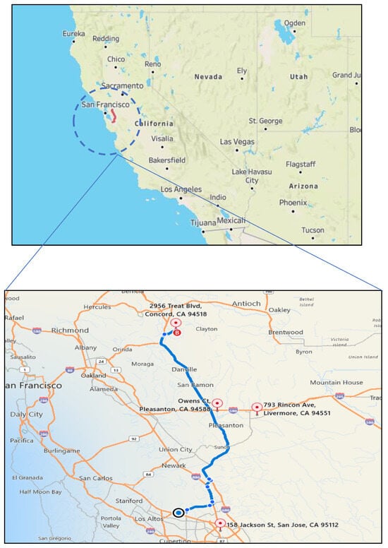
Figure 1.
Map of the study area with red points indicating the selected four monitoring stations for local PM2.5.
The vehicle used in this study is a Nissan Rogue S, a 2023 model compact SUV that is 100% gas and has a cabin air filter, with a passenger volume of 2.98 m3 (105.4 cu. ft.) [31]. This study aimed to investigate the relationship between in-vehicle PM2.5 concentrations and ambient (local) PM2.5 concentrations obtained from the local monitoring stations. Advanced statistical analyses were performed to study the impact of various parameters on PM, and data visualization techniques were utilized to represent the pollutant concentration data from both sensors. Furthermore, the study explored the buildup of carbon dioxide (CO2) inside the vehicle under different ventilation conditions, as well as the correlation between vehicle speed and PM concentrations.
For data collection during the commute, the sensors were positioned inside the vehicle, on the dashboard. This placement was chosen since this is a stable location around the breathing zone. Two ventilation conditions were tested to investigate the CO2 buildup in vehicles. RC on is when the vehicle’s cabin recirculation mode is activated. This mode circulates the cabin air internally, preventing fresh air intake from outside. For newer vehicles, RC on is oftentimes automatically set when using air conditioning, to save energy. RC off is when the vehicle’s cabin recirculation mode is deselected, which allows fresh air intake into the cabin from outside through air filters.
Based on sensor performance studies from the South Coast Air Quality Management District (AQMD) [32,33,34,35]. PM2.5, PM10, and CO2 data from the Temtop M2000 were used for analysis, while the GPS coordinate data were taken from the Flow 2 sensor.
A trip was considered a one-way commute from Sunnyvale to Walnut Creek or the other way around. PM2.5, PM10, CO2, and GPS were simultaneously measured for each trip, and data was recorded every minute by the sensors and statistically analyzed as daily, monthly, and seasonally to capture temporal variations. Trip data were taken from May 2023 to December 2023, which spanned almost four seasons: spring included May, summer included June to August, fall included September to November, and winter included December.
A study indicated that the on-road air quality can contribute 30% of in-vehicle PM2.5 [10] exposure. Therefore, it is worthwhile to study the correlation between PM2.5 levels inside and outside of vehicles. In this study, the ambient PM2.5 concentrations were used to represent on-road PM2.5 concentrations. The local (ambient air) PM2.5 concentrations were obtained from the EPA database. The four local PM2.5 monitoring stations chosen are San Jose-Jackson, Pleasanton-Owens Ct, Livermore, and Concord (Figure 1), all owned and operated by the Bay Area Air Quality Management District (https://www.baaqmd.gov/, accessed 15 September 2024).
Statistical analysis (such as the average and standard deviation of trips) and regression of the data were mainly performed with Microsoft Excel. For data visualization, Tableau was used to develop box plots and commute maps with PM concentrations.
3. Results
3.1. Temporal Variation of Particulate Matter
The average in-vehicle PM concentrations for morning and evening rush hours are summarized in Table 2 and Table 3 respectively. These values are all lower than the US EPA’s National Ambient Air Quality Standards (NAAQS) of 35 µg/m3 (24-h average). Frequently, the morning PM concentrations were higher compared to evenings, and this is consistent with studies of [9,11]. This may be attributed to the higher humidity in the mornings and subsequent absorption of moisture around the particles, which affects portable laser-based monitoring devices the most [36,37]. In a study by Kim et al. [36], the PM increased with increasing RH up to 70% RH. When RH > 70%, steam particles combined, forming water drops, decreasing PM concentrations. Such a trend of higher morning in-vehicle PM concentrations than evening warrants more studies in the future.
Table 2.
Summary of in-vehicle particulate matter for morning rush hours.
Table 3.
Summary of in-vehicle particulate matter for evening rush hours.
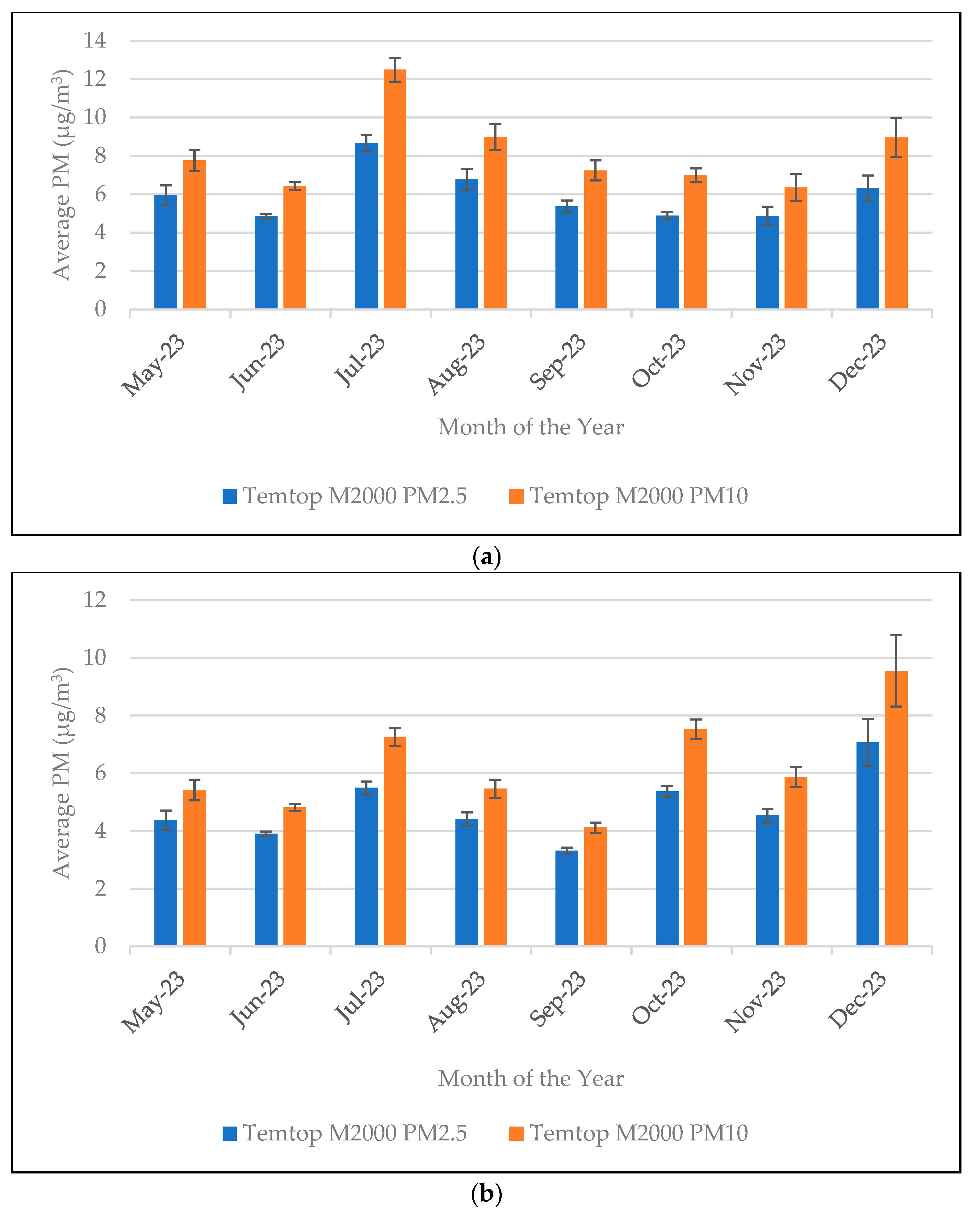
Analyzing the morning peak data from Temtop M2000, the PM2.5 and PM10 were higher for summer, followed by spring and fall. The measured PM concentrations are comparable with those from Sacramento, CA [8], which is in the same state but are lower than those reported in Taipei, which used a similar Temtop device [12].
Figure 2 shows monthly in-vehicle PM concentrations in the form of average and 95% confidence interval (CI) for morning and evening rush hour data. The higher in-vehicle PM concentrations observed in July and August are likely related to higher temperatures and congestion from lane closure due to tree removal along I-680 [38]. Figure 3 displays maps of PM concentrations to the coordinates of the commute. These trip-based concentration maps can identify hotspots of higher in-vehicle exposure for specific trips and can also be helpful for traffic management or source reduction.
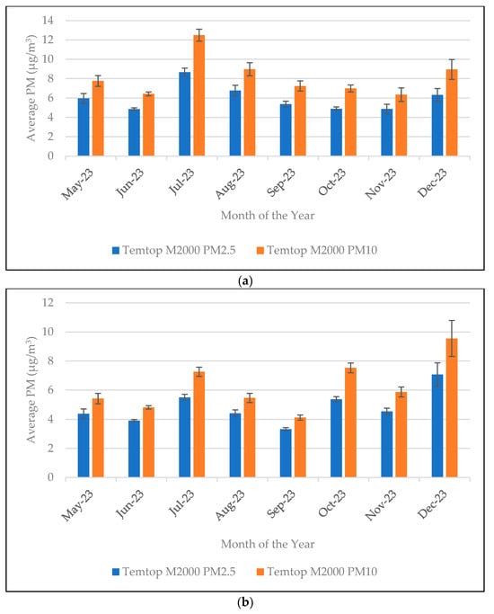
Figure 2.
Monthly variation of in-vehicle PM concentrations (a) morning rush hours; (b) evening rush hours. In both graphs error bars represent 95% CI.
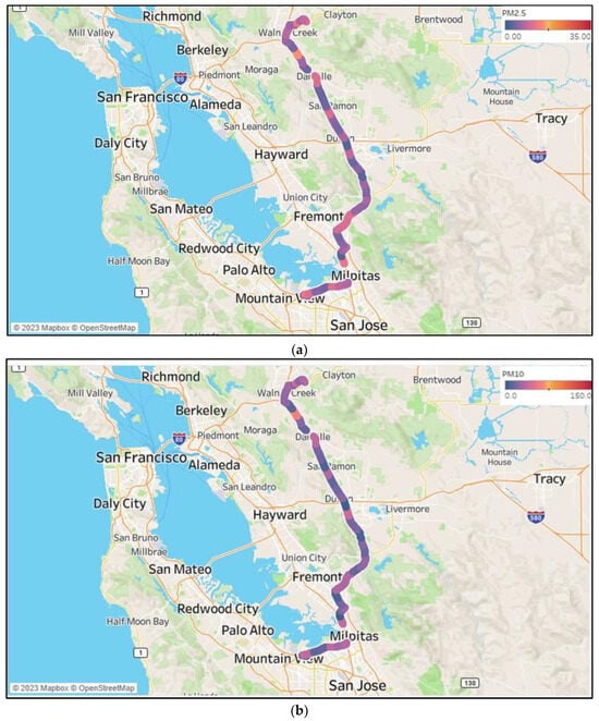
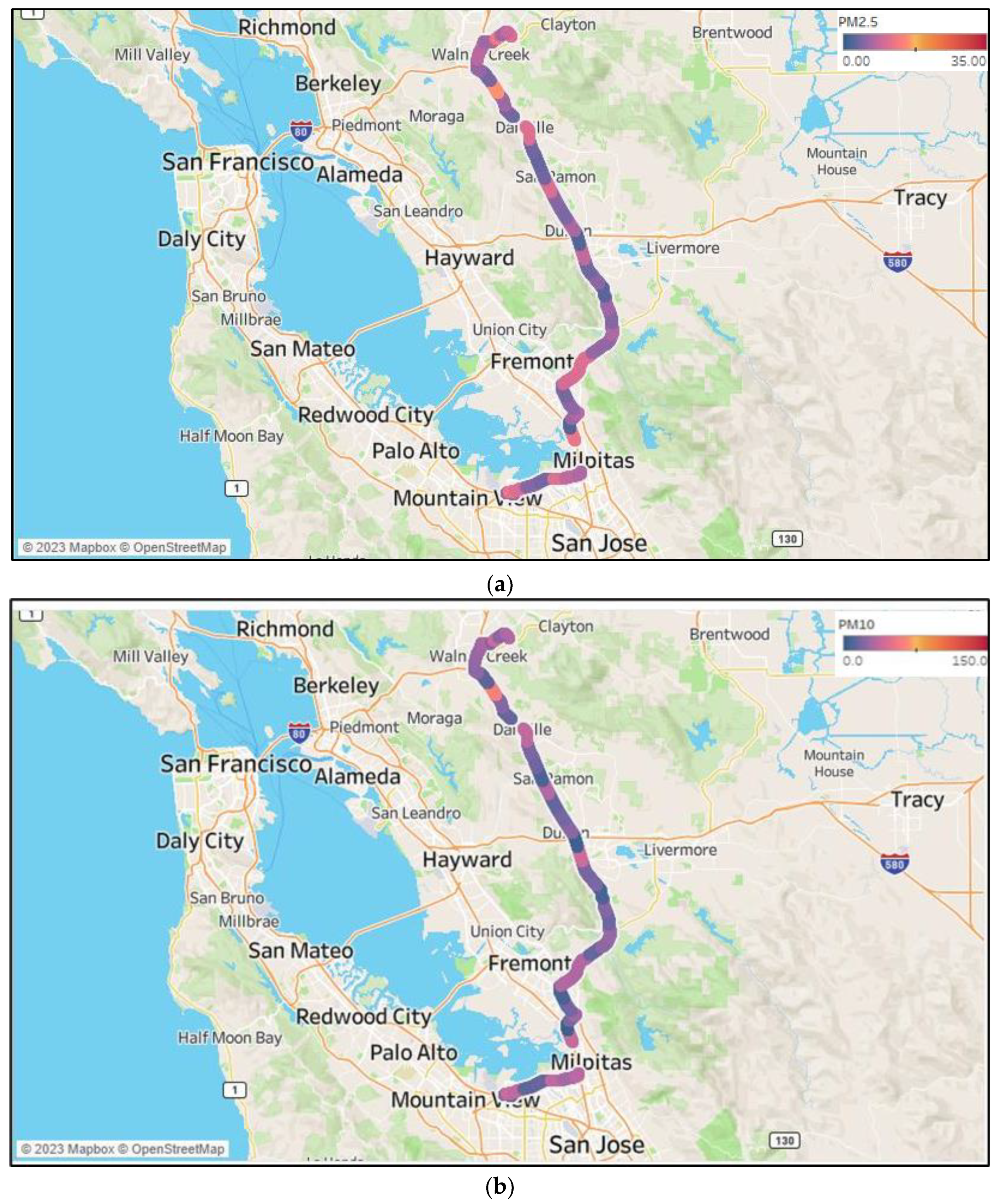
Figure 3.
PM distributions from Sunnyvale to Walnut Creek on 25 May 2023 for morning rush hours (a) PM2.5 (b) PM10.
Color-coded PM concentrations along a trip were plotted in Figure 3. The trip in Figure 3 is a morning trip with RC on; the ambient local PM2.5 for that trip was 4.33 µg/m3, and ambient humidity was 79%. For this particular trip, the average in-vehicle PM2.5 recorded was 5.19 µg/m3 and PM10 was 6.02 µg/m3. As seen from the figures, higher PM concentrations were observed while crossing cities such as Fremont, Pleasanton, Dublin, and San Ramon, which are predominantly residential communities with local businesses, and higher traffic was observed in these areas due to people commuting to and from work.
3.2. Relationship between In-Vehicle PM2.5 and Local PM2.5 Concentrations
To obtain the PM2.5 local concentrations, the concentrations measured at the four monitoring stations—namely San Jose-Jackson, Pleasanton-Owens Ct, Livermore, and Concord—were averaged according to the commute time. Of these stations, Pleasanton-Owens Ct is a near-road site and is a Special Purpose Monitor (SPM) [39], while the other three are State or Local Air Monitoring Stations (SLAMS) [39].
For example, for a trip from 7:30 a.m. to 8:30 a.m. on a given day, the local PM2.5 at the four stations was selected and averaged from 7:00 a.m. to 9:00 a.m. as the local PM2.5 concentration for that trip.
The correlation between in-vehicle and ambient PM2.5 was also plotted in Figure S1, with fitting parameters in Table S1 in the Supplementary Material. Non-linear correlation showed a better fit, while the exponential fitting seemed to be the closest.
To further analyze in-vehicle exposure to outside PM2.5, the ratio of inside/outside (Y′) was computed using average in-vehicle PM2.5 and average local PM2.5 concentrations of each trip [40]. The fraction (Y′ − 1) quantifies the fraction by which in-vehicle PM2.5 exceeds (or is less than) PM2.5 local [40]. In this study, 68% of in-vehicle PM2.5 values are lower than the corresponding ambient values. This may be a result of the air filters in the vehicle. The ratio Y′ for in-vehicle PM2.5 from Temtop M2000 ranged from 0.29–2.09, with an average of 0.92.
For the whole data set, scatter plots were created, and logarithmic, exponential, and linear trendline equations were fitted (Figure 4) to the data using an 80/20 training-testing approach [41].
Y′ = In-vehicle PM2.5/Local PM2.5
Y′ − 1 = (In-vehicle PM2.5 − Local PM2.5)/Local PM2.5
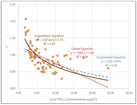
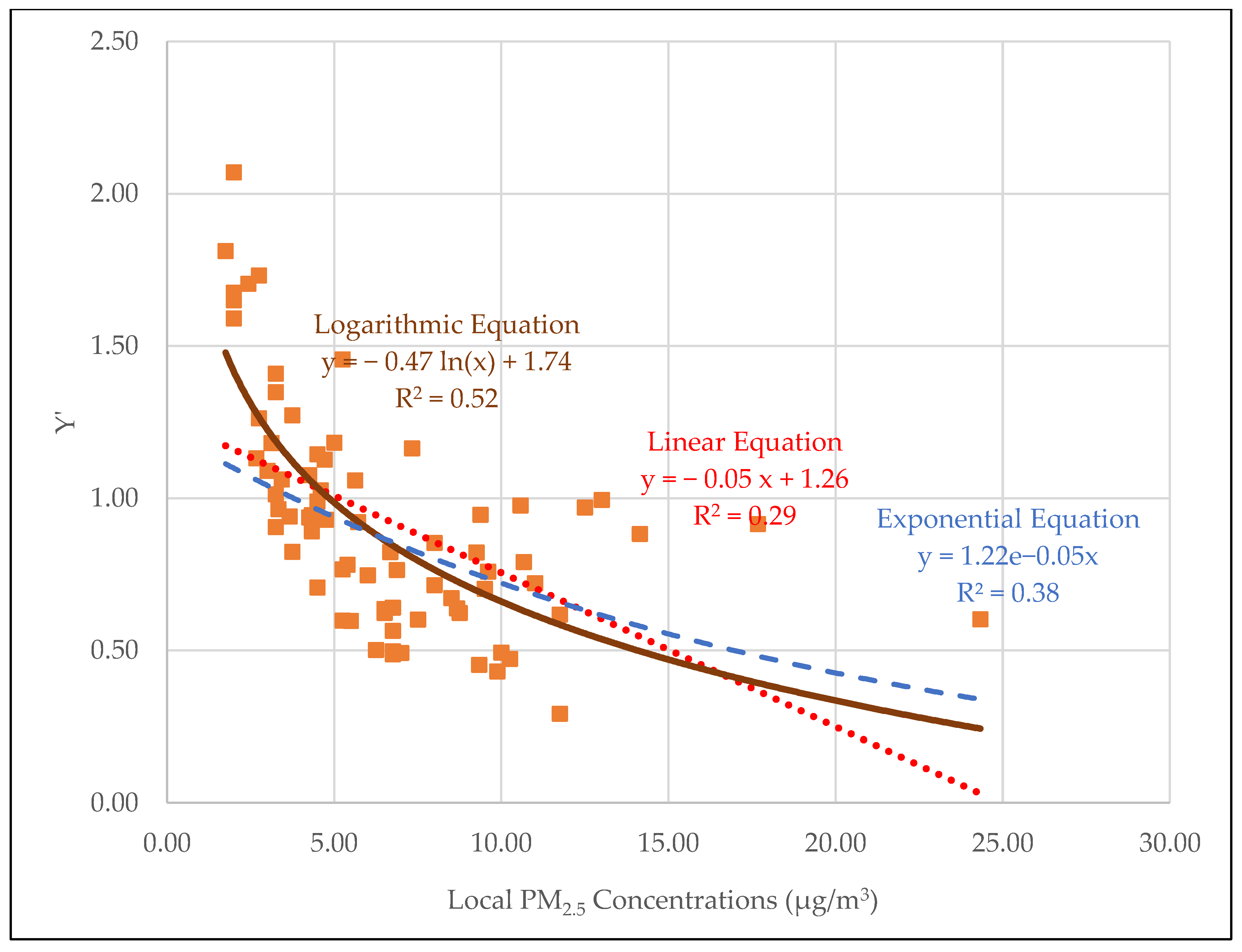
Figure 4.
Regression for Y′ vs. local PM2.5 concentrations based on Temtop M2000 data.
The logarithmic, exponential, and linear curves were plotted with 80% training data and tested on the remaining 20% of the data (local PM2.5 vs. Y′). Evaluation metrics such as root mean square error (RMSE) and mean absolute percentage error (MAPE) were calculated for all the curve fittings (Table 4). For Temtop M2000, though the logarithmic curve showed lower RMSE and MAPE compared to the exponential, the exponential curve was selected to have unit compatibility and have a better fit even for higher local PM2.5 concentrations.
Table 4.
RMSE and MAPE for logarithmic, exponential, and linear fittings of PM2.5.
The exponential fitting suggests that the ratio of in-vehicle to ambient PM2.5 does not increase or decrease linearly with changing ambient levels. Instead, the relationship follows a non-linear pattern, which could arise from factors such as vehicle ventilation dynamics, traffic influences, or nonlinear atmospheric processes affecting the relationship between indoor and outdoor particulate levels as ambient concentrations vary. The non-linear correlation is also reported by Goel et al. [40]. However, their study reported a logarithmic correlation between the ratio of in-vehicle to ambient PM2.5 concentrations and ambient PM2.5 concentrations.
3.3. CO2 Buildup In-Vehicles
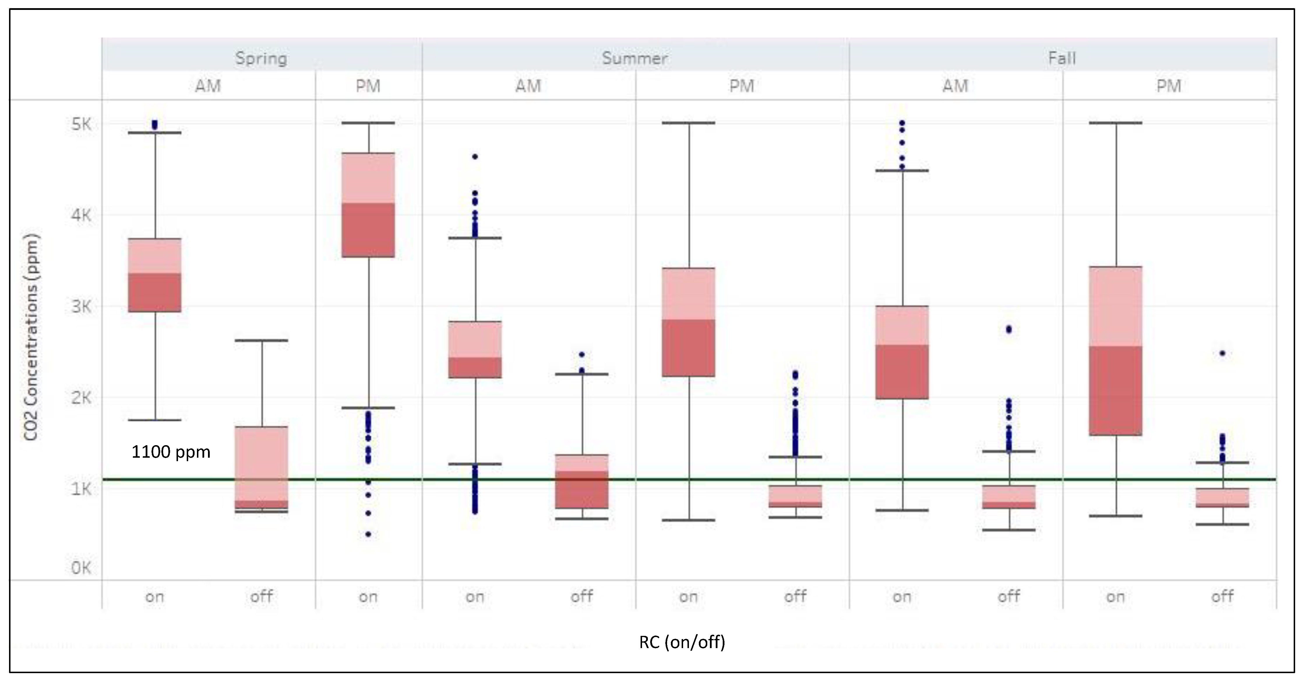
Figure 5 presents the CO2 concentrations with RC on and off for both morning and evening trips for four seasons (See also Table S2 in supplementary material). Across all the seasons, whether morning (AM) or evening (PM) rush hour, the CO2 concentrations were significantly higher when the RC was on compared to RC off. Spring season recorded the highest CO2 (exceeding 3000 ppm), particularly during evening hours with RC on. Summer, Fall, and Winter recorded similar CO2 levels during morning and evenings with slight variations. When RC was on, CO2 levels were 2.11–2.86 times higher than RC off. This difference highlights the substantial buildup of CO2 that can occur in the confined vehicle cabin environment when the recirculation mode is selected. Maintaining adequate fresh air ventilation is crucial for keeping in-vehicle CO2 concentrations at acceptable levels and reducing their negative impacts on driver comfort and cognitive performance during long commutes. With fresh air intake, the CO2 levels are largely within the 1100 ppm guidelines set by ASHRAE [18].
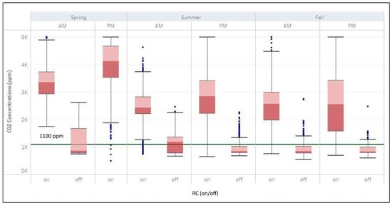
Figure 5.
Seasonal in-vehicle CO2 concentrations during morning (am) and evening (pm) rush hours with RC on and RC off.
Furthermore, as shown in Table S2, when RC was on, higher CO2 concentrations were observed in the evening than in the morning for three seasons measured: spring, summer, and fall. This is likely due to the higher temperatures in the evening rush hours (than mornings) and the accumulation of CO2 throughout the day inside the vehicle cabin. In comparison, when RC was off, higher CO2 concentrations were observed during the morning rush hours for summer, fall, and winter. This is consistent with the diurnal cycle of CO2 concentrations, which peak in the morning and are at their lowest in the afternoon [42]. By not using the recirculation mode, the average CO2 concentrations are mostly within the ASHRAE guideline. Letting fresh air in is especially helpful for keeping healthy levels of CO2 during long or congested commutes. The control of CO2 concentrations is largely the choice of vehicle occupants, while the choice of ventilation settings is associated with energy use. For BEVs, this can be a challenge due to the competition between personal comfort and vehicle range.
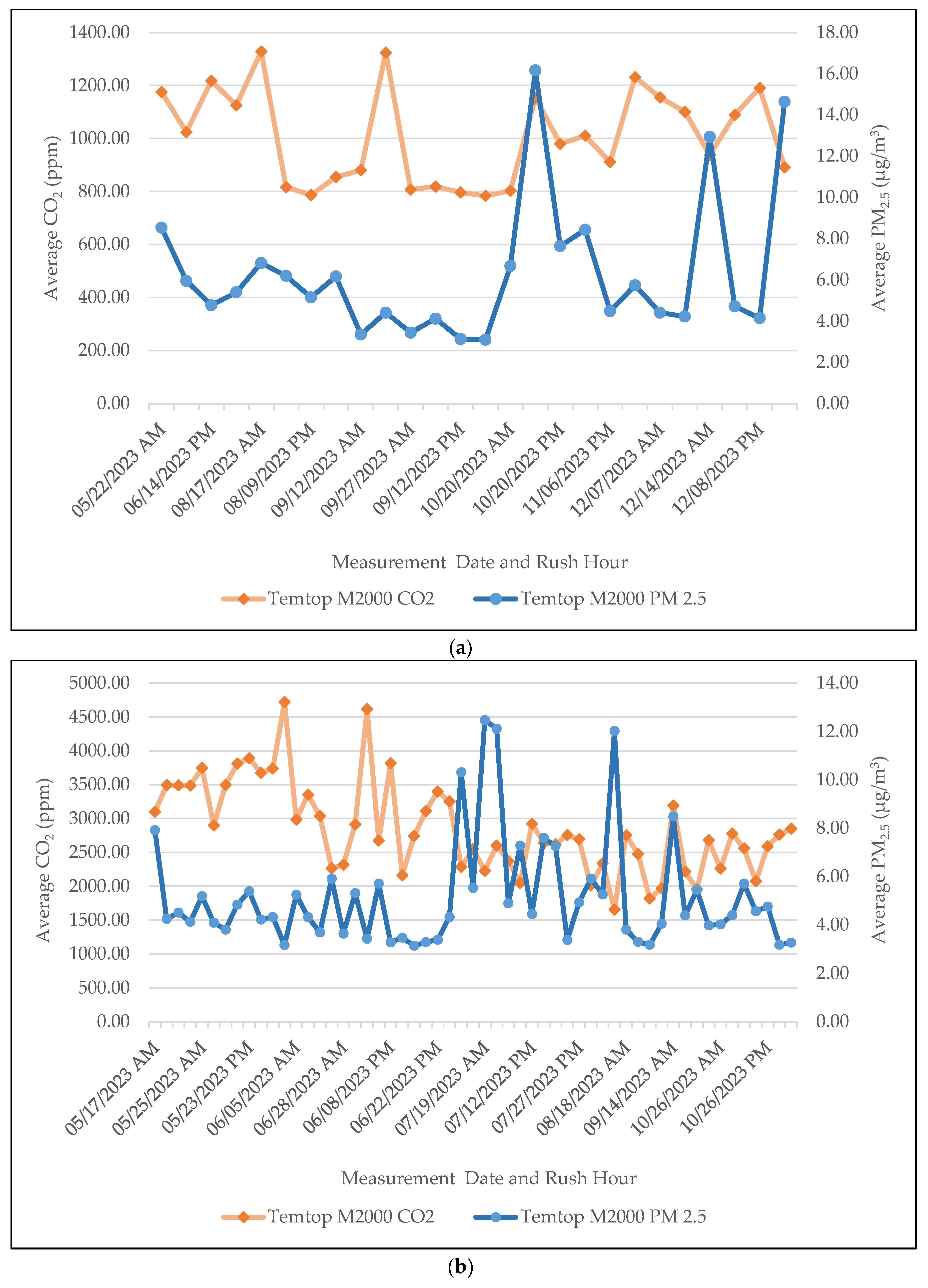
Figure 6 below displays the aggerated data of in-vehicle CO2 together with PM2.5 for both RC on and RC off conditions. In Figure 6a with RC off, the CO2 concentrations range from 784 ppm to 1328 ppm, with an average of 1007 ppm. In-vehicle PM2.5 levels range from 3.09 μg/m3 to 16.16 μg/m3, with an average of 6.33 μg/m3.
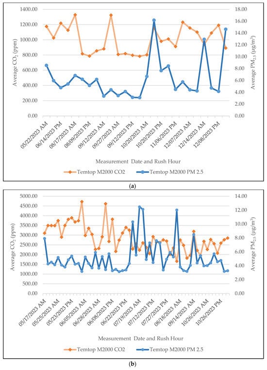
Figure 6.
Temporal plots of CO2 and PM2.5 with (a) RC off; and (b) RC on conditions.
In comparison, in Figure 6b with RC on, the CO2 concentrations range from 1656 ppm to 4718 ppm, with an average of 2851 ppm. In-vehicle PM2.5 levels range from 3.14 μg/m3 to 12.47 μg/m3, with an average of 5.16 μg/m3.
In this study, RC on mode resulted in rapid CO2 build-up to 5000 ppm at max in some of the trips. Under RC off conditions, with fresh air coming into the vehicle, CO2 concentrations were greatly reduced. The average CO2 levels were 2.11–2.86 times higher at RC on compared to RC off. The RC off mode is recommended to keep the levels of CO2 within the ASHRAE guidelines. In our study, in-vehicle PM2.5 levels with RC on are mostly lower than that of RC off, which is in agreement with studies [8,9,10]. However, higher PM2.5 levels were observed in a few of our trips during RC on. One such is included in Figure S2. This is likely due to the high ambient PM2.5 concentrations.
3.4. Speed vs. In-Vehicle Particulate Matter Concentrations
Some studies indicated that higher in-vehicle PM concentrations can be associated with congestion, which can be indicated by reduced speed [9,10]. This seems to be also reflected by the trip-based pollution graphs, such as Figure 3. Therefore, the vehicle speed during the commute was calculated from distance using the Haversine Formula [43], with the latitudes and longitudes from the Flow 2 sensor.
where, lat 1, lat 2—latitude 1 and latitude 2, long 1, long 2—longitude 1 and longitude 2.
Distance (in miles) = a cos (cos (radians(90 − lat1)) × cos (radians(90 − lat2)) + sin(radians(90 − lat1)) × sin(radians(90 − lat2)) × cos (radians(long1 − long2))) × 3958.756
The vehicle speed can then be averaged for the whole trip. The correlation of vehicle speed and PM was studied for select trips in each month and during both AM and PM rush hours, as shown in Table 5. The correlation coefficient (R) between vehicle speed and in-vehicle PM (both PM2.5 and PM10) is largely weakly positive, consistent with that of the Birmingham, UK, study [10].
Table 5.
The correlation between vehicle speed and in-vehicle PM.
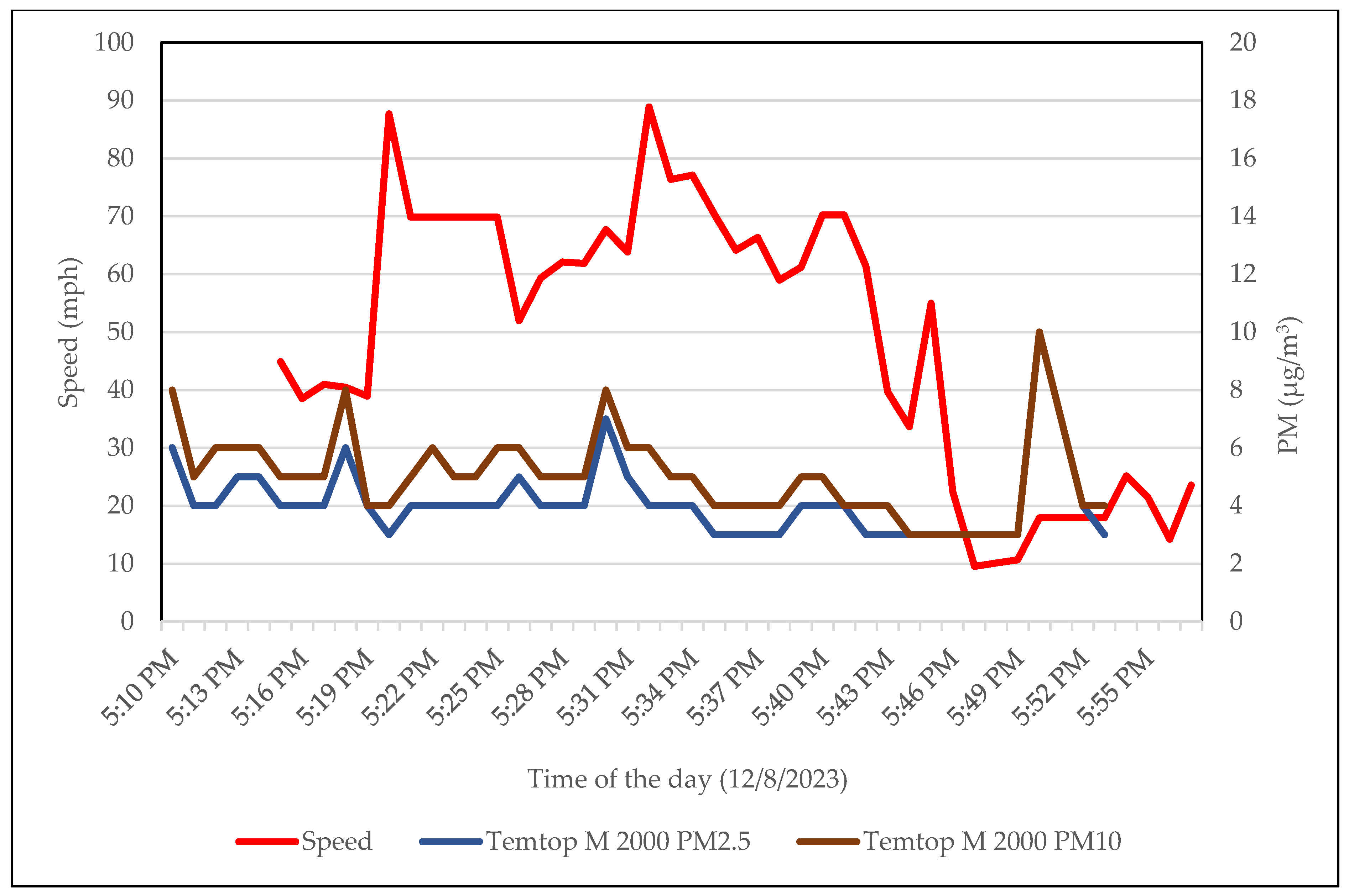
Figure 7 below displays the speed vs. PM concentrations on 8 December 2023. Throughout the commute, the average speed maintained by the vehicle was 78.90 km/h (49 mph) on the highway, (where the speed limit is 104.60 km/h (65 mph)) without air conditioning and with circulation from outside (RC off). During the beginning of the trip for the first 10 min, the vehicle maintained a relatively low average speed of 65.98 km/h (41 mph). During this period, the average PM2.5 concentration was 4.60 μg/m3. Subsequently, at 5:20 p.m., the congestion eased, and the vehicle’s speed increased, averaging 109.44 km/h (68 mph) for the next 23 min until 5:42 p.m. Throughout this higher-speed segment, the average PM2.5 observed was at 3.90 μg/m3. Following this, the vehicle’s speed was significantly reduced due to congestion, with an average of 37.01 km/h (23 mph) for the remainder of the trip. However, the average PM2.5 concentration was 4.00 μg/m3. It was during this lower-speed segment that an elevated PM2.5 concentration of 10 μg/m3 was recorded at 5:50 p.m.
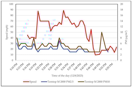
Figure 7.
Speed and PM concentrations on 8 December 2023—evening rush hour.
The correlation coefficient (R) between vehicle speed and in-vehicle PM2.5 was −0.12, indicating a weak negative correlation. This suggested that slow speed has some correlation with PM2.5 increase. The correlation coefficient (R) for vehicle speed and PM10 was 0.14, indicating a weak positive correlation. A study in the same state but a larger city (Los Angeles) indicated that brake and dust particles were in the PM10 range [44]. Speed reduction is expected to be negatively correlated to PM10 due to increased brake and tire abrasion, but this was not observed in this study, or from another study [10]. This warrants further investigation.
In the mornings, traffic jams tend to occur on the local roads of Walnut Creek after I-680 is exited. During the evening rush hour, the lower vehicle speed was due to higher traffic in evenings compared to mornings, and the areas with lower vehicle speeds are Pleasanton-Livermore areas; exit from I-680 to enter I-880. Minutes after the low speed, when the vehicle starts moving, high PM concentrations were observed likely due to the movement of vehicles ahead generating more PM.
Similar analyses were also performed for multiple trips. Overall, the correlation between vehicle speed and in-vehicle PM2.5 and PM10 concentrations was generally weak, with correlation coefficients (R) ranging from −0.12 to 0.32 across different trips. While some instances of PM spikes coincided with reductions in vehicle speed, there were also cases where elevated PM levels occurred despite constant speeds. Spikes in PM concentrations were sometimes observed after sudden reductions in vehicle speed, potentially due to the resuspension of settled particles or outside air intake. Lower vehicle speeds may be associated with higher in-vehicle PM levels in some cases, potentially due to reduced dispersion and dilution, as well as the presence of vehicular traffic. The results from this study suggest that vehicle speed may be one of many contributors to in-vehicle PM concentrations [9,10].
4. Conclusions
In Vehicle exposure to air pollutants during rush hour commutes in the San Francisco Bay area, CA, was studied with two low-cost sensors. Each trip length is about 80.5 km (50 miles), mostly on the highway with commute times of about an hour, with windows closed. The seasonal in-vehicle PM2.5 during morning rush hours varied from 5.07 µg/m3 to 6.55 µg/m3, and PM2.5 concentrations during evening rush hours were in the range of 4.38 µg/m3 to 4.47 µg/m3. Overall, in-vehicle PM2.5 concentrations are much lower than EPA’s NAAQS’ 24-h average concentration of 35 µg/m3, and 68% of these are lower than the corresponding ambient values (values observed at the state monitoring stations) [45]. Seasonal variations of in-vehicle PM2.5 were evident during the morning rush hour, with the highest in summer and lowest in the fall, while those during the evening rush hour did not exhibit strong variations. Higher PM2.5 levels during the morning rush hour than evening rush hour were consistently observed for all four seasons studied. PM10 largely follows the trend of PM2.5. In this study, an exponential relationship was found between the PM2.5 concentration ratios of in-vehicle vs. ambient/local (Y′) with local PM2.5 concentrations. The average CO2 level with the cabin recirculation mode engaged (RC on) was 2851 ppm for two occupants, while it decreased to 1007 ppm under the fresh air mode. In contrast, the average PM2.5 concentration was 5.16 µg/m3 with RC on and 6.33 µg/m3 at RC off. This research demonstrates the effectiveness of using low-cost sensors for real-time monitoring of in-vehicle air quality. The findings provide valuable insights into the dynamics of air pollution within vehicles, emphasizing the importance of maintaining adequate ventilation and monitoring air quality to reduce health risks.
5. Limitations
The portable devices used in this study may be affected by temperature, relative humidity, and other environmental conditions since these devices do not have the sophisticated conditioning mechanisms of the FEM/FRM grade devices [27]. Although the Temtop M2000 has been regarded as fairly accurate [32,33,34], we did not do side-by-side calibration with FEM devices in this study. Low-cost devices, though very convenient in operation and usage, have limitations and uncertainties that should be estimated and compared with standard instruments [46]. The uncertainty of the low-cost devices may affect observations with small differences. This study only investigated windows closed conditions, which lacks dynamic range compared with other studies. This study did not simultaneously measure ambient air and cabin air at the same location due to the limited number of instruments and used the average ambient PM2.5 concentrations from 4 local monitoring stations. This approximation can introduce inaccuracies in the correlation estimates. Using one sensor outside and one sensor inside the vehicle should be considered in future studies.
Supplementary Materials
The following supporting information can be downloaded at: https://www.mdpi.com/article/10.3390/atmos15091130/s1. Figure S1. Regression for In-vehicle PM2.5 Vs Local PM2.5 Concentrations. Figure S2. Temporal Plots of CO2 and PM2.5 on Select Days with (a) RC On and (b) RC Off. Table S1. RMSE and MAPE for Logarithmic, Exponential, and Linear fittings. Table S2. Seasonal Average CO2 Concentrations with RC On and Off.
Author Contributions
Conceptualization, M.L. and R.D.; methodology, M.L. and R.D.; experiments, data collection, and analysis, R.D.; writing—original draft preparation, R.D. and M.L.; writing—review and editing, M.L. and R.D.; project administration, M.L.; funding acquisition, M.L. All authors have read and agreed to the published version of the manuscript.
Funding
This research was funded by the Ohio Bureau of Workers’ Compensation (OBWC) for funding (WSIC24-230331-027).
Institutional Review Board Statement
Not applicable.
Informed Consent Statement
Informed consent was obtained from all subjects involved in the study.
Data Availability Statement
Most of the data used in this paper are published in the form of thesis, conferences, and journal papers. The data presented in this study are available upon request. The data are not publicly available due to privacy.
Acknowledgments
The authors thank Jun Wang for his support as the lead PI of this project and Alyssa Yerkeson for her help.
Conflicts of Interest
The authors declare no conflicts of interest. The funders had no role in the design of the study, in the collection, analysis, or interpretation of data, in the writing of the manuscript, or in the decision to publish the results.
References
- Mukund, R.; Kelly, T.J.; Spicer, C.W. Source Attribution of Ambient Air Toxic and Other VOCS in Columbus, Ohio. Atmos. Environ. 1996, 30, 3457. [Google Scholar] [CrossRef]
- Aarnio, P.; Yli-Tuomi, T.; Kousa, A.; Mäkelä, T.; Hirsikko, A.; Hämeri, K.; Räisänen, M.; Hillamo, R.; Koskentalo, T.; Jantunen, M. The concentrations and composition of and exposure to fine particles (PM2.5) in the Helsinki subway system. Atmos. Environ. 2005, 39, 5059–5066. [Google Scholar] [CrossRef]
- Aggarwal, S.G.; Kumar, S.; Mandal, P.; Sarangi, B.; Singh, K.; Pokhariyal, J.; Mishra, S.K.; Agarwal, S.; Sinha, D.; Singh, S.; et al. Traceability Issue in PM2.5 and PM10 Measurements. Mapan—J. Metrol. Soc. India 2013, 28, 153–166. [Google Scholar] [CrossRef]
- Fast Facts on Transportation Greenhouse Gas Emissions. Available online: https://www.epa.gov/greenvehicles/fast-facts-transportation-greenhouse-gas-emissions (accessed on 22 August 2024).
- Li, C.; Managi, S. Contribution of on-road transportation to PM2.5. Sci. Rep. 2021, 11, 21320. [Google Scholar] [CrossRef]
- Wu, T.G.; Chen, Y.D.; Chen, B.H.; Harada, K.H.; Lee, K.; Deng, F.; Rood, M.J.; Chen, C.C.; Tran, C.T.; Chien, K.L.; et al. Identifying low-PM2.5 exposure commuting routes for cyclists through modeling with the random forest algorithm based on low-cost sensor measurements in three Asian cities. Environ. Pollut. 2022, 294, 118597. [Google Scholar] [CrossRef]
- Kim, W.; Anorve, V.; Tefft, B.C. American Driving Survey, 2014–2017. 2019. Available online: https://trid.trb.org/View/1590683 (accessed on 15 September 2024).
- Ham, W.; Vijayan, A.; Schulte, N.; Herner, J.D. Commuter exposure to PM2.5, BC, and UFP in six common transport microenvironments in Sacramento, California. Atmos. Environ. 2017, 167, 335–345. [Google Scholar] [CrossRef]
- Kumar, P.; Hama, S.; Nogueira, T.; Abbass, R.A.; Brand, V.S.; de Fatima Andrade, M.; Asfaw, A.; Aziz, K.H.; Cao, S.; El-Gendy, A. In-car particulate matter exposure across ten global cities. Sci. Total Environ. 2021, 750, 141395. [Google Scholar] [CrossRef]
- Matthaios, V.N.; Harrison, R.M.; Koutrakis, P.; Bloss, W.J. In-vehicle exposure to NO2 and PM2.5: A comprehensive assessment of controlling parameters and reduction strategies to minimise personal exposure. Sci. Total Environ. 2023, 900. [Google Scholar] [CrossRef]
- De Nazelle, A.; Fruin, S.; Westerdahl, D.; Martinez, D.; Ripoll, A.; Kubesch, N.; Nieuwenhuijsen, M. A travel mode comparison of commuters’ exposures to air pollutants in Barcelona. Atmos. Environ. 2012, 59, 151–159. [Google Scholar] [CrossRef]
- Wang, C.; Lim, B.; Wang, Y.; Huang, Y.T. Identification of high personal PM2.5 exposure during real time commuting in the Taipei metropolitan area. Atmosphere 2021, 12, 396. [Google Scholar] [CrossRef]
- California Tops US EV Adoption: 25% EV Share of Total Sales In H1 2023. Available online: https://insideevs.com/news/688779/california-tops-us-ev-adoption-25-percent-share-total-sales-h1-2023/ (accessed on 28 August 2024).
- California Moves to Accelerate to 100% New Zero-Emission Vehicle Sales by 2035. Available online: https://ww2.arb.ca.gov/news/california-moves-accelerate-100-new-zero-emission-vehicle-sales-2035#:~:text=The%20rule%20establishes%20a%20year-by-year%20roadmap%20so%20that,set%20out%20in%20Governor%20Newsom%E2%80%99s%20Executive%20Order%20N-79-20. (accessed on 28 August 2024).
- Ewing, J. President Biden Sets a Goal of 50 Percent Electric Vehicle Sales by 2030. NewYork Times 2021. Available online: https://www.nytimes.com/2021/08/05/business/biden-electric-vehicles.html (accessed on 28 August 2024).
- Timmers, V.R.; Achten, P.A. Non-exhaust PM emissions from electric vehicles. Atmos. Environ. 2016, 134, 10–17. [Google Scholar] [CrossRef]
- Muratori, L.; Peretto, L.; Pulvirenti, B.; Di Sante, R.; Bottiglieri, G.; Coiro, F. Optimal Control of Air Conditioning Systems by Means of CO2 Sensors in Electric Vehicles. Sensors 2022, 22, 1190. [Google Scholar] [CrossRef] [PubMed]
- Ventilation for Acceptable Indoor Air Quality. 2016. Available online: https://www.ashrae.org/File%20Library/Technical%20Resources/Standards%20and%20Guidelines/Standards%20Addenda/62.1-2016/62_1_2016_d_20180302.pdf (accessed on 15 July 2024).
- EPA Indoor Air Quality—Website. Available online: https://www.epa.gov/indoor-air-quality-iaq/can-i-measure-carbon-dioxide-co2-indoors-get-information-ventilation (accessed on 2 July 2024).
- Satish, U.; Mendell, M.J.; Shekhar, K.; Hotchi, T.; Sullivan, D.; Streufert, S.; Fisk, W.J. Is CO2 an indoor pollutant? Direct effects of low-to-moderate CO2 concentrations on human decision-making performance. Environ. Health Perspect 2012, 120, 1671–1677. [Google Scholar] [CrossRef] [PubMed]
- Hudda, N.; Fruin, S.A. Carbon dioxide accumulation inside vehicles: The effect of ventilation and driving conditions. Sci. Total Environ. 2018, 610, 1448–1456. [Google Scholar] [CrossRef] [PubMed]
- Lee, E.S.; Zhu, Y. Application of a high-efficiency cabin air filter for simultaneous mitigation of ultrafine particle and carbon dioxide exposures inside passenger vehicles. Environ. Sci. Technol. 2014, 48, 2328–2335. [Google Scholar] [CrossRef] [PubMed]
- Lohani, D.; Barthwal, A.; Acharya, D. Predictive Modelling of In-vehicle CO2 Concentration using Sensor Data Analytics. In Proceedings of the 2018 IEEE SENSORS, New Delhi, India, 28–31 October 2018; pp. 1–4. [Google Scholar]
- Lohani, D.; Barthwal, A.; Acharya, D. Modeling vehicle indoor air quality using sensor data analytics. J. Reliab. Intell. Environ. 2022, 8, 105–115. [Google Scholar] [CrossRef]
- D’Eon, J.C.; Stirchak, L.T.; Brown, A.S.; Saifuddin, Y. Project-Based Learning Experience That Uses Portable Air Sensors to Characterize Indoor and Outdoor Air Quality. J. Chem. Educ. 2021, 98, 445–453. [Google Scholar] [CrossRef]
- Williams, R. Findings from the 2013 EPA Air Sensors Workshop2013. Available online: https://19january2017snapshot.epa.gov/air-research/findings-2013-epa-air-sensors-workshop.html (accessed on 7 June 2024).
- Woodall, G.M.; Hoover, M.D.; Williams, R.; Benedict, K.; Harper, M.; Soo, J.C.; Jarabek, A.M.; Stewart, M.J.; Brown, J.S.; Hulla, J.E.; et al. Interpreting mobile and handheld air sensor readings in relation to air quality standards and health effect reference values: Tackling the challenges. Atmosphere 2017, 8, 182. [Google Scholar] [CrossRef]
- Temtop M2000 2nd Generation—Air Quality Monitor with Data Export. Available online: https://temtopus.com/products/temtop-m2000-2nd-generation-air-quality-monitor-for-pm2-5-pm10-particles-co2-hcho-temperature-humidity-settable-audio-alarm-data-export-recording-curve-easy-calibration?variant=40587983421488 (accessed on 7 June 2024).
- Flow 2, by Plume Labs: The First Smart Air Quality Tracker. Available online: https://plumelabs.com/en/flow/ (accessed on 6 June 2024).
- Qiu, Z.; Cao, H. Commuter exposure to particulate matter in urban public transportation of Xi’an, China. J. Environ. Health Sci. Eng. 2020, 18, 451–462. [Google Scholar] [CrossRef]
- Nissan Rogue Specifications. Available online: https://www.caranddriver.com/nissan/rogue/specs/2023/nissan_rogue_nissan-rogue_2023 (accessed on 2 July 2024).
- Temtop M2000 Evaluation Summary—South Coast AQMD. Available online: http://www.aqmd.gov/docs/default-source/aq-spec/summary/elitech-temtop-m2000-2nd-generation---summary-report.pdf?sfvrsn=8 (accessed on 12 June 2024).
- Temtop M2000 Field Evaluation Report. Available online: http://www.aqmd.gov/aq-spec/sensordetail/elitech---temtop-m2000 (accessed on 12 June 2024).
- Temtop M2000—Laboratory Evaluation Report. Available online: http://www.aqmd.gov/aq-spec/sensordetail/elitech---temtop-m2000 (accessed on 12 June 2024).
- Flow 2 Evaluation Report by South Coast AQMD. Available online: http://www.aqmd.gov/docs/default-source/aq-spec/field-evaluations/plume-labs-flow-2---field-evaluation.pdf?sfvrsn=8 (accessed on 12 June 2024).
- Kim, H.; Kim, J.; Roh, S. Effects of Gas and Steam Humidity on Particulate Matter Measurements Obtained Using Light-Scattering Sensors. Sensors 2023, 23, 6199. [Google Scholar] [CrossRef]
- Jayaratne, R.; Liu, X.; Thai, P.; Dunbabin, M.; Morawska, L. The influence of humidity on the performance of a low-cost air particle mass sensor and the effect of atmospheric fog. Atmos. Meas. Tech. 2018, 11, 4883. [Google Scholar] [CrossRef]
- Southbound I-680 Lane Closures Between San Ramon and Sunol at Various Locations for Tree Removal May 29-Late August 2023. 2023. Available online: https://dot.ca.gov/caltrans-near-me/district-4/d4-news/2023-05-16-sb-680-tree-work (accessed on 7 June 2024).
- 2024 Annual Air Monitoring Network Plan. Available online: https://www.baaqmd.gov/en/news-and-events/page-resources/2024-news/052024-amnp (accessed on 5 June 2024).
- Goel, R.; Gani, S.; Guttikunda, S.K.; Wilson, D.; Tiwari, G. On-road PM2.5 pollution exposure in multiple transport microenvironments in Delhi. Atmos. Environ. 2015, 123, 129–138. [Google Scholar] [CrossRef]
- Gholamy, A.; Kreinovich, V.; Kosheleva, O. Why 70/30 or 80/20 Relation Between Training and Testing Sets: A Pedagogical Explanation. Int. J. Intell. Technol. Appl. Stat. 2018, 11, 105–111. [Google Scholar] [CrossRef]
- Hou, H.; Zhang, S.; Ding, Z.; Wang, Y.; Yang, Y.; Guo, S. Temporal variation of near-surface CO2 concentrations over different land uses in Suzhou City. Environ. Earth Sci. 2016, 75, 1197. [Google Scholar] [CrossRef]
- Haversine Formula for Computing Speed. Available online: https://andyarthur.org/haversine-formula-in-ecel.html (accessed on 9 June 2024).
- Oroumiyeh, F.; Zhu, Y. Brake and tire particles measured from on-road vehicles: Effects of vehicle mass and braking intensity. Atmos. Environ. X 2021, 12, 100121. [Google Scholar] [CrossRef]
- California Air Resources Board—Particulate Matter. Available online: https://ww2.arb.ca.gov/resources/inhalable-particulate-matter-and-health (accessed on 9 June 2024).
- Hofman, J.; Peters, J.; Stroobants, C.; Elst, E.; Baeyens, B.; Van Laer, J.; Spruyt, M.; Van Essche, W.; Delbare, E.; Roels, B. Air quality sensor networks for evidence-based policy making: Best practices for actionable insights. Atmosphere 2022, 13, 944. [Google Scholar] [CrossRef]

Disclaimer/Publisher’s Note: The statements, opinions and data contained in all publications are solely those of the individual author(s) and contributor(s) and not of MDPI and/or the editor(s). MDPI and/or the editor(s) disclaim responsibility for any injury to people or property resulting from any ideas, methods, instructions or products referred to in the content. |
© 2024 by the authors. Licensee MDPI, Basel, Switzerland. This article is an open access article distributed under the terms and conditions of the Creative Commons Attribution (CC BY) license (https://creativecommons.org/licenses/by/4.0/).