Article

Spatio-Temporal Analysis of Drought with SPEI in the State of Mexico and Mexico City

by
Mauricio Carrillo-Carrillo
1,*,
Laura Ibáñez-Castillo
2,*,
Ramón Arteaga-Ramírez
2 and
Gustavo Arévalo-Galarza
3
1
Chapingo Autonomous University, Postgraduate Degree in Agricultural Engineering and Integral Water Use, Texcoco C.P. 56230, Mexico
2
Department of Irrigation, Autonomous University of Chapingo, Texcoco C.P. 56230, Mexico
3
Department of Soils, Autonomous University of Chapingo, Texcoco C.P. 56230, Mexico
*
Authors to whom correspondence should be addressed.
Atmosphere 2025, 16(2), 202; https://doi.org/10.3390/atmos16020202
Submission received: 15 December 2024 / Revised: 7 February 2025 / Accepted: 8 February 2025 / Published: 11 February 2025

Abstract

:
Climate change and increasing water demand are causing supply problems in Mexico City and the State of Mexico. The lack of complete and up-to-date meteorological information makes it difficult to understand and analyze climate phenomena such as droughts. Climate Engine provides decades of climate data to analyze such changes. These data were used to calculate SPEI (Standardized Precipitation-Evapotranspiration index) at scales of 1, 3, 6, 9, 12, and 24 months between 1981 and 2023 in the study area. The Standard Normal Homogeneity Test (SNHT) indicated greater homogeneity in temperature data, while precipitation data exhibited potential inhomogeneities. The Mann–Kendall test showed no significant trend for precipitation but a clear increasing trend in temperature. Droughts have become more frequent and severe over the last decade, particularly in the western State of Mexico and the southwest of Mexico City. The wettest years within the last 14 years were 2010, 2015, and 2018, while the most severe droughts occurred in 2017, 2019, 2020, 2021, and 2023. The findings suggest intensifying drought conditions, likely driven by rising temperatures and climate variability. These trends emphasize the need for improved water resource management and adaptation strategies to mitigate the growing impact of droughts in central Mexico.

1. Introduction

The duration of droughts could last from months to longer periods like years, but it can critically threaten the water availability in a hydrological system [1]. The negative consequences could affect a wide range of social, economic, and environmental sectors [2]. This recurrent phenomenon is caused by a lack of precipitation [3,4] and meaningfully can be the root of decreases in crop yields, particularly through critical plant growth stages for instance germination, pollination, and grain filling [5,6,7].
The recent technological development of remote sensing techniques and instruments for the spatial monitoring of variables related to the hydrological cycle has made it possible to refine their spatial and temporal resolution, which has resulted in their use as sources of information for drought analysis. This has allowed the creation of drought monitoring and assessment systems at different spatial scales (e.g., regional, national, global). Such systems integrate observations derived from different sources of information (e.g., remote sensing, ground-based radars, gauging stations, etc.) with results from climatological, hydrological, and land surface models [8]. From this, it is possible to identify affected regions, and response protocols are activated once an event has started [9].
There is a certain difficulty in the measurement of the severity of a drought, given that we normally recognize a drought by the consequence of its effects on agriculture, water resources, ecology, forest fires, economic losses, etc., but there is no specific physical variable that allows us to measure the harshness of the drought. Therefore, it is challenging to identify when a drought begins and ends, as well as to keep track of its duration, magnitude, and surface extension [9,10]. Droughts can be separated into four categories, which are meteorological drought, agricultural drought, hydrological drought, and socio-economic drought. The drought indices are accessible for examining conditions of regional drought. Over the last few decades, the development of many outstanding drought indices has been widely used for drought observation [11].
Drought indices are vital for objectively quantifying and comparing the severity, duration, and extent of drought in regions with varying climatic and hydrological regimes. The Standardized Precipitation Index (SPI), described by McKee [12] and Guttman [13], measures normalized anomalies in precipitation. It has been recommended as a main indicator of drought by the World Meteorological Organization [14] and has a universal meteorological index of drought by the Lincoln Declaration on Drought [15].
Most drought indices currently used are applicable for the identification and measurement of dry and wet conditions on monthly scales. Droughts can be monitored and forecasted on a monthly scale, too. The escalating frequency of unusually high temperatures and droughts due to global warming [16,17] originates in sudden droughts [18,19].
In Mexico, droughts are monitored with the SPI index [20], which is a meteorological index. This index, regardless of the extensive approval, only considers precipitation as an atmospheric variable for its calculations. SPI leaves out other variables that may affect drought intensity, like temperature, wind speed, and humidity. To confront this obstacle, Vicente-Serrano [21] developed SPEI. It uses a similar calculation but instead regulates differences in the cumulative climatic water balance, which is defined as the difference between precipitation and potential evapotranspiration. The simple water balance approach of SPEI provides a more accurate and realistic measure of drought. While maintaining the computational simplicity of a meteorological index, SPEI effectively accounts for the water balance in a region by incorporating evapotranspiration, an essential factor in areas where vegetation covers the soil, particularly in agricultural fields. SPEI is more relevant than SPI in agricultural areas, without the added complexity of a dedicated agricultural index. Previous research in certain regions of Mexico has demonstrated that SPEI excels at detecting both maximum and minimum drought conditions that SPI is unable to identify [22,23].
Climatic information is necessary to comprehend climatic phenomena, for example, rainfall measurements from established ground-based weather stations, which are the main origin of such climatic statistics. Nonetheless, historical track records from these stations are ineffective in many places around the world because of the scarce, decreasing, or non-existent network of stations. For this reason, rainfall information derived from satellite products has been used more frequently to replace missing data from stations of observation [24]. New technologies have provided a complete or just partial but sufficient solution to complement the lack of information, extending to areas that, due to time and budget issues, would not have been possible to analyze [25].
The State of Mexico and Mexico City face a scarcity of water resources due to the increase in water demand (population growth) and its inefficient use (infrastructure in poor condition and without adequate maintenance). This problem is increased by the effects of climate change that causes low rainfall and recurrent drought phenomena in recent years [26]. The objective of this work is to use weather databases to be able to calculate the SPEI indices for the State of Mexico and Mexico City for a period from 1981 to 2023, using the CHIRPS databases to obtain precipitation data and DAYMET to obtain temperature data. Analyzing the evolution of such weather variables and their effects on the values of drought indicators provides a better understanding of the effects of human activities and their toll on the environment and its social and economic importance.

2. Materials and Methods

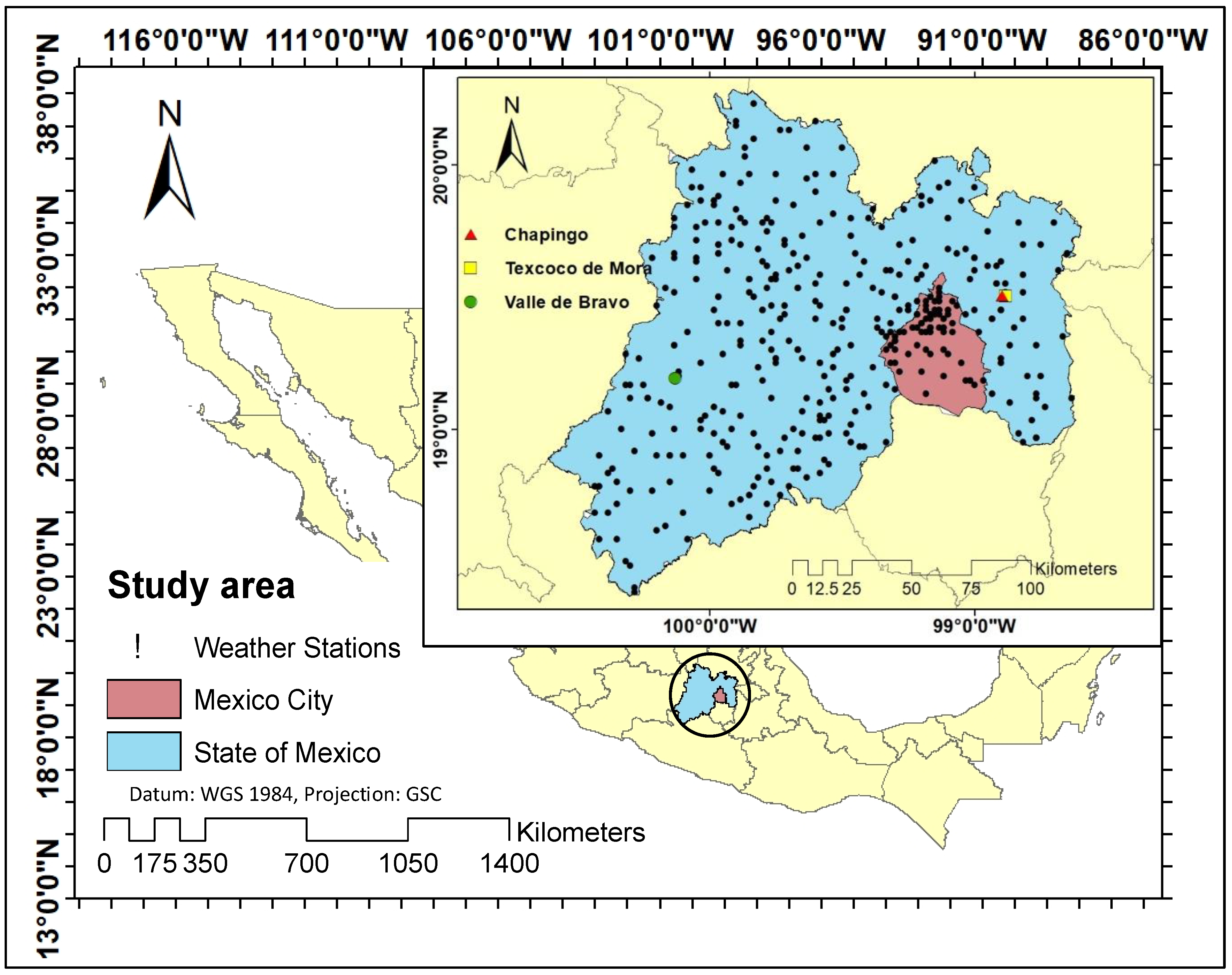
2.1. Description of the Study Area

The study area covers the State of Mexico and Mexico City (Figure 1). The State of Mexico has an area of 22,351.8 km2, which represents 1.1% of Mexico’s surface area; however, it is the most populated state with 16,992,418 inhabitants. Mexico City (CdMx) has an area of 1494.3 km2, which represents 0.1% of the country’s surface; Mexico City has 9,209,944 inhabitants [27]. The study area is located between 2250 and 2750 m above sea level, and the predominant climate is dry temperate, with an average annual temperature of 15.9 °C and an average annual rainfall of 686 mm, with a climate known as sub-humid temperate [28].

2.2. Climatological Databases

In total, 381 meteorological stations from the National Meteorological System (SMN) station network (Figure 1) were analyzed in Mexico City and the State of Mexico for a period from January 1981 to December 2023 (42 years).
The availability of stations still operating is 59% in the study area; for this reason, the geographic coordinates of each meteorological station served as a reference for the recovery of climatic data in Climate Engine (http://ClimateEngine.org (accessed on 9 September 2024)). It was decided to consider the CHIRPS database that presents daily, pentad, and monthly data. Data were collected from the DAYMET database, which provides daily and monthly values. When comparing the monthly CHIRPS and DAYMET data for station 15,170 in Chapingo (Figure 1) with the monthly observed data, R2 = 0.8921 was obtained for precipitation, R2 = 0.9974 for the maximum temperature, and R2 = 0.9824 for the minimum temperature.

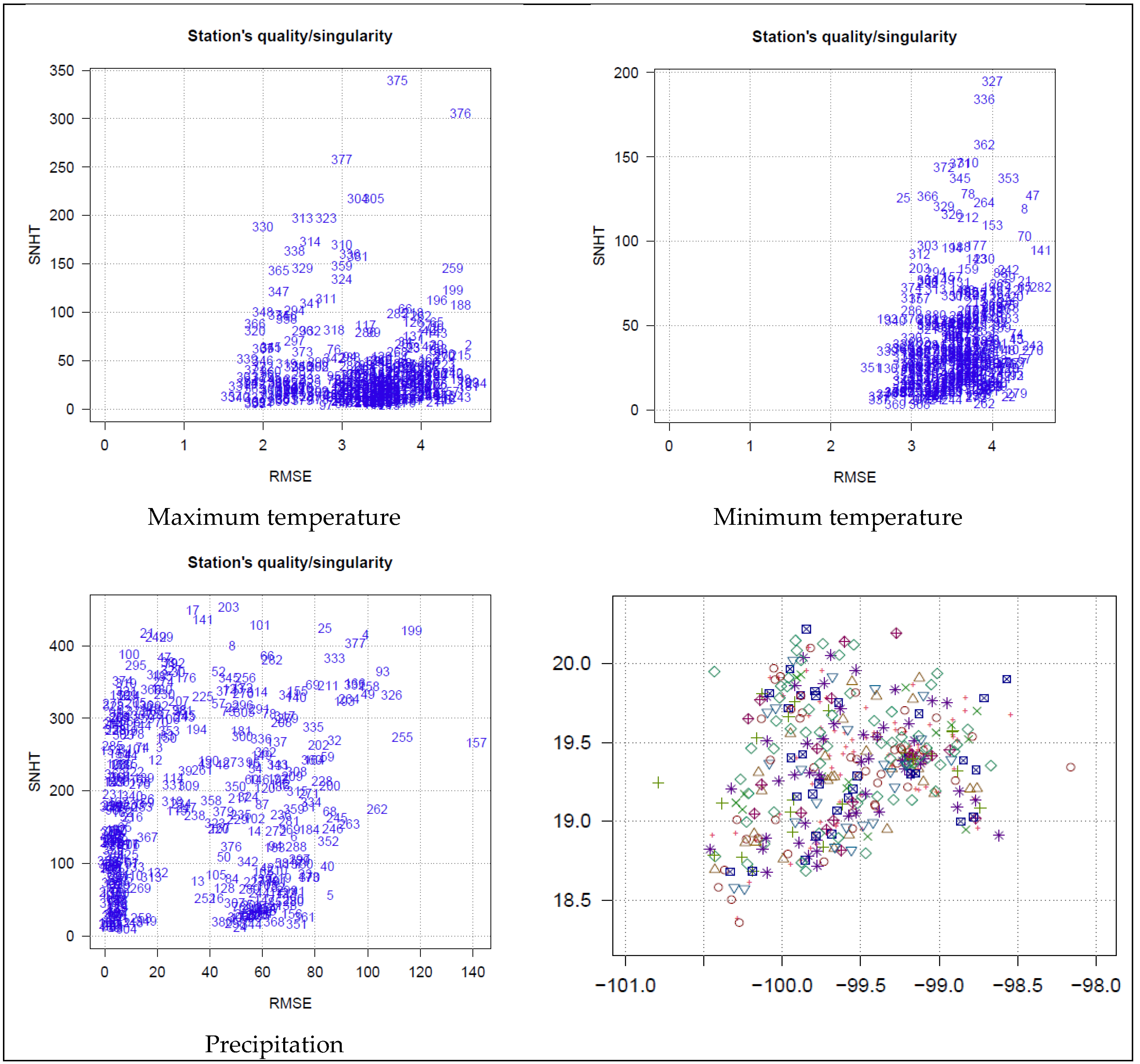
2.3. Climatol: Software for the Validation and Analysis of Climate Data

Climatol is a software tool designed for the validation, detection, and correction of errors in climate data time series. It offers functionalities for quality control, homogenization, and missing data filling of climatological series, as well as tools to generate climatological summaries and grids from the results [29].
Among its key functions, Climatol includes advanced methods for outlier detection, which identify anomalous values or measurement errors in weather station records. The software also provides tools for the correction of missing data, using interpolation techniques and information from neighboring stations. These capabilities are crucial for maintaining the consistency of time series and avoiding distortions in climate analysis [30].
Furthermore, Climatol conducts statistical validation of data series, assessing their internal consistency and identifying potential inconsistencies over time. This process allows users to detect and correct irregularities before utilizing the data in more in-depth studies, such as climate trend analysis or the evaluation of extreme weather events [31].

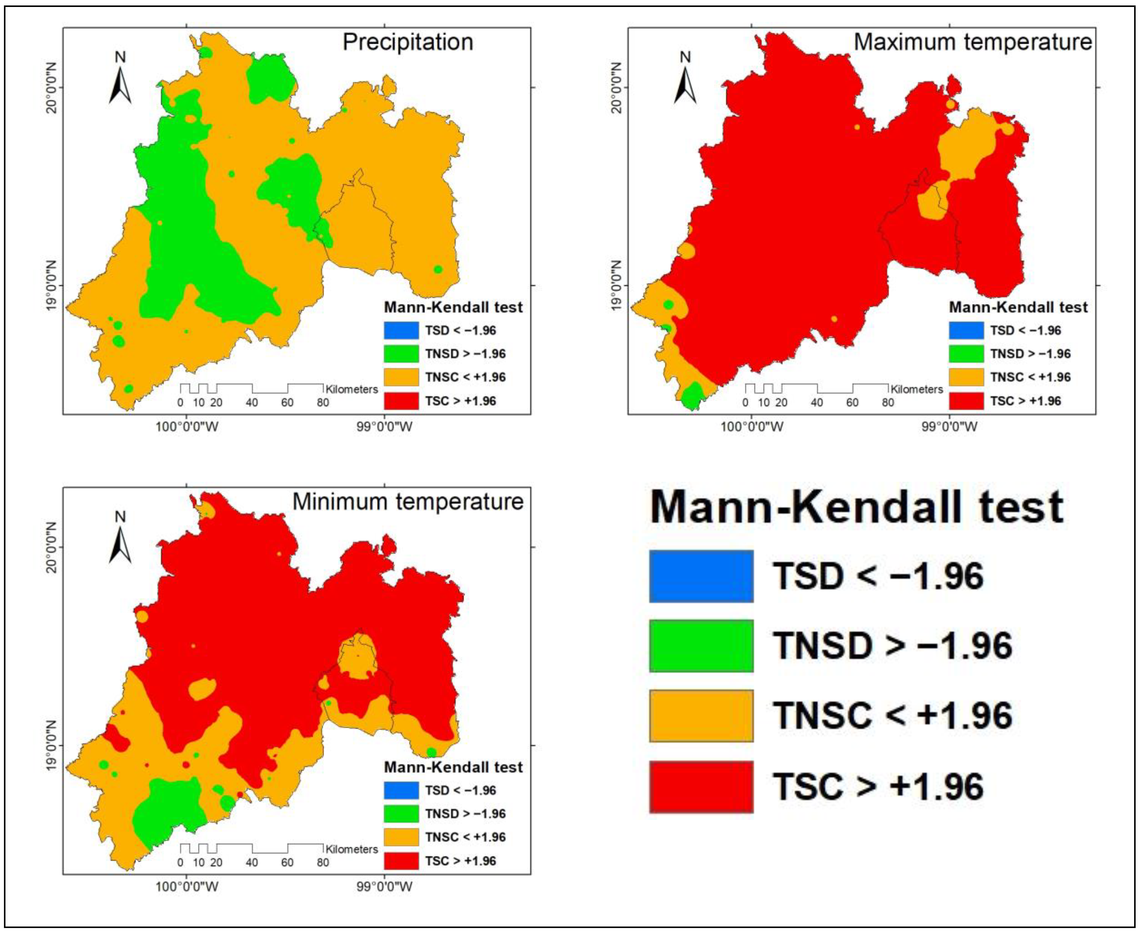
2.4. Mann–Kendall Statistical Test

The statistical characteristics of the hydrological series, such as the mean, standard deviation, and serial correlation coefficients, are affected when the series shows a trend in the mean or variance or when decreasing or increasing jumps occur. In general, the presence of a positive or negative trend on climate variables is induced by human activities, such as deforestation, opening of new cultivation areas, rectification of riverbeds, construction of reservoirs, and reforestation. It is also a product of sudden natural processes, such as forest fires, earthquakes, landslides, and volcanic eruptions.
HydroGeoLogic [32] considers that the Mann–Kendall test is the most suitable method for analyzing trends in the climatological series. Also, this method allows detecting and locating the approximate starting point of a given trend. The Mann–Kendall test is a non-parametric test [33,34], suggested to evaluate the trend in environmental data series [35]. This test basically consists of the comparison between the values that compose the same time series in sequential order [36].
If the number of positive pairs is P, and the number of negative pairs is N, then S is defined as S = P − N. For n > 10, a Z statistic can be defined that follows the standard normal distribution, where Equation (1) represents the Mann–Kendall test statistic:
Z = S 1 n ( n 1 ) ( 2 n + 5 ) 18   i f   S > 0 0   i f   S = 0 S + 1 n ( n 1 ) ( 2 n + 5 ) 18   i f   S < 0
The result of S indicates the possible existence of trends if the value of S is significantly different from zero. With S being different from zero, the null hypothesis H0 can be rejected, and the alternative hypothesis H1 would be accepted [34].

2.5. Climate Engine

Climate Engine (https://app.climateengine.org) grants non-commercial users of any scientific level to take advantage of cloud storage capabilities to collect Earth observation data. Also, it can show how climate change has affected landscapes over the past decades, and it is able to quantitatively analyze years of information in a matter of seconds. It was launched with the support of the White House Climate Data Initiative and the Google Faculty Research award, has a key role in Earth science research, and helps decision-making for government agencies worldwide and for users that trust its information [37].

2.6. CHIRPS Satellite Data

There are three main sources for the main data for the CHIRPS algorithm: (1) the Climate Hazards group precipitation climatology (CHPclim), which employs global precipitation at 0.05° latitude/longitude resolution that is estimated for each month from station data, averaged satellite observations, elevation, latitude, and longitude [38,39]; (2) satellite precipitation estimated from thermal infrared precipitation (IRP); and (3) in situ rain gauge measurements. What differentiates CHPclim from other precipitation climatology is that it uses long-term satellite mean precipitation fields as a model to obtain climatological data. This improves its performance in mountainous countries [39].
Additional data from certain regions, such as East Africa, Central America, and Afghanistan, are also used [25,40]. This method for merging CHIRP with station observations applies to the expected correlation between the precipitation of a given pixel and that of nearby stations. These correlations are approximated from the CHIRP fields. An additional correlation value is also used, which is supposed to be an estimation of the correlation between the real precipitation at each pixel and the CHIRP values [41].
The combination of station statistics with CHIRP data is performed on two different time scales, the pentad (5-day) and monthly, afterwards re-scaling the pentads to a daily level. The preliminary CHIRPS is accessible after the end of five days, and the final version is generated by the third week of next month.

2.7. DAYMET Satellite Data

DAYMET estimates daily weather and climate variables by interpolating and extrapolating land observations by using a statistical modeling technique. These meteorological variables are the daily minimum and maximum temperatures, precipitation, vapor pressure, shortwave radiation, snow water equivalent, and day length produced over a 1 km × 1 km gridded area [42]. Once there is an absence of ground information, the Daymet method uses a combination of interpolation and extrapolation, applying data from several instrumented locations and certain weights for each location that refer to the spatial and temporal relationships of the estimation location to instrumental observations. The number of instrumental observations used for each estimation is determined as a parameter for each of the primary variables of the DAYMET.
When the station density is very low, a series of modifications in the algorithm is applied to improve the sturdiness of the data; it leaves the iterative calculations of the station density and instead outlines the search of the radius for each estimation location that is sized exactly to capture the average number of involved stations based on pre-computed matrices of inter-station distances. The primary DAYMET output variables are produced from two distinct workflows: one for the daily temperature variables and one for the daily precipitation variable that comes from preprocessed input station observations and precomputed station lists and interpolation weights for each estimation grid location [42].

2.8. Potential Evapotranspiration Equations (PETs)

Certain precautions were carried out to select the best applied potential evapotranspiration methods that extend the choice of equation types, which include equations based on temperature, radiation, and combined equations [43]. In order of complexity, these models are Thornthwaite [44], Hargreaves [45], Penman–Montieth with the Hargreaves (P-M) radiation [46], Priestley–Taylor [47], and FAO-56 Penman–Montieth referenced here as P-M (FAO-56) [46]. The FAO-56 reference crop definition [43] is used for all the PET models, except for the Thornthwaite equation, which uses the original definition of Thornthwaite [44].
The Thornthwaite method is distinctive because it is based on an empirical relationship between mean monthly temperature and potential evapotranspiration [48,49]; this method was included because it was cited in the original SPEI methodology and is commonly used [21]. The rest of the PET methods follow the general form, Equation (2):
P E T = R n + γ · m a s s   t r a n s f e r   t e r m + γ
where Rn represents the net radiation, γ is the psychrometric constant, and Δ is the slope of the vapor saturation–pressure vs. temperature curve at the given air temperature. Another equation is Hargreaves that uses daily difference between maximum temperature and minimum temperature as an alternative for estimating the radiation [45] and simplifies the mass transfer term with a constant. The P-M equation (Hargreaves) uses an identical estimate of radiation but evaluates mass transfer using wind speed from the Watch Forcing Dataset [50].

2.9. Drought Indices

According to NIDIS, 2025 [51], a drought is “a deficiency of precipitation over an extended period of time (usually a season or more), resulting in a water shortage”. Scientists have defined several types of drought: (a) meteorological drought, (b) hydrological drought, (c) agricultural drought, (d) socioeconomic drought, and (e) ecological drought. The meteorological drought is based on the calculus of a deficiency of precipitation, and the other drought indices are the product of the cascade effects of this deficiency. We are working with a meteorological index called SPEI. We describe some of the meteorological drought indices.

2.9.1. The Palmer Drought Severity Index (PDSI)

This method was a pioneer for the development of drought indices; it measures humidity as a positive value and dryness as a negative value, which are obtained from the supply and demand of the water balance equation that considers previous precipitation, moisture, runoff, and evaporation demand at a ground level. It had some problems that were solved by developing a self-calibration PDSI (sc-PDSI) [52] that is spatially similar to extreme wet and dry events with predicted frequencies in their values for infrequent conditions.

2.9.2. Standardized Precipitation Index (SPI)

It is a widely used drought index that measures precipitation anomalies over different timescales, as proposed by McKee [12] and shown in Equation (3), where precipitation (xi) from the mean for a specified time (xj) is divided by the standard deviation (σ).
S P I = x i x j σ
Each of the datasets are fitted to the Gamma distribution. SPI is calculated for different time scales, i.e., 1, 3, 6, 9, 12, 24, and 48 months [53].

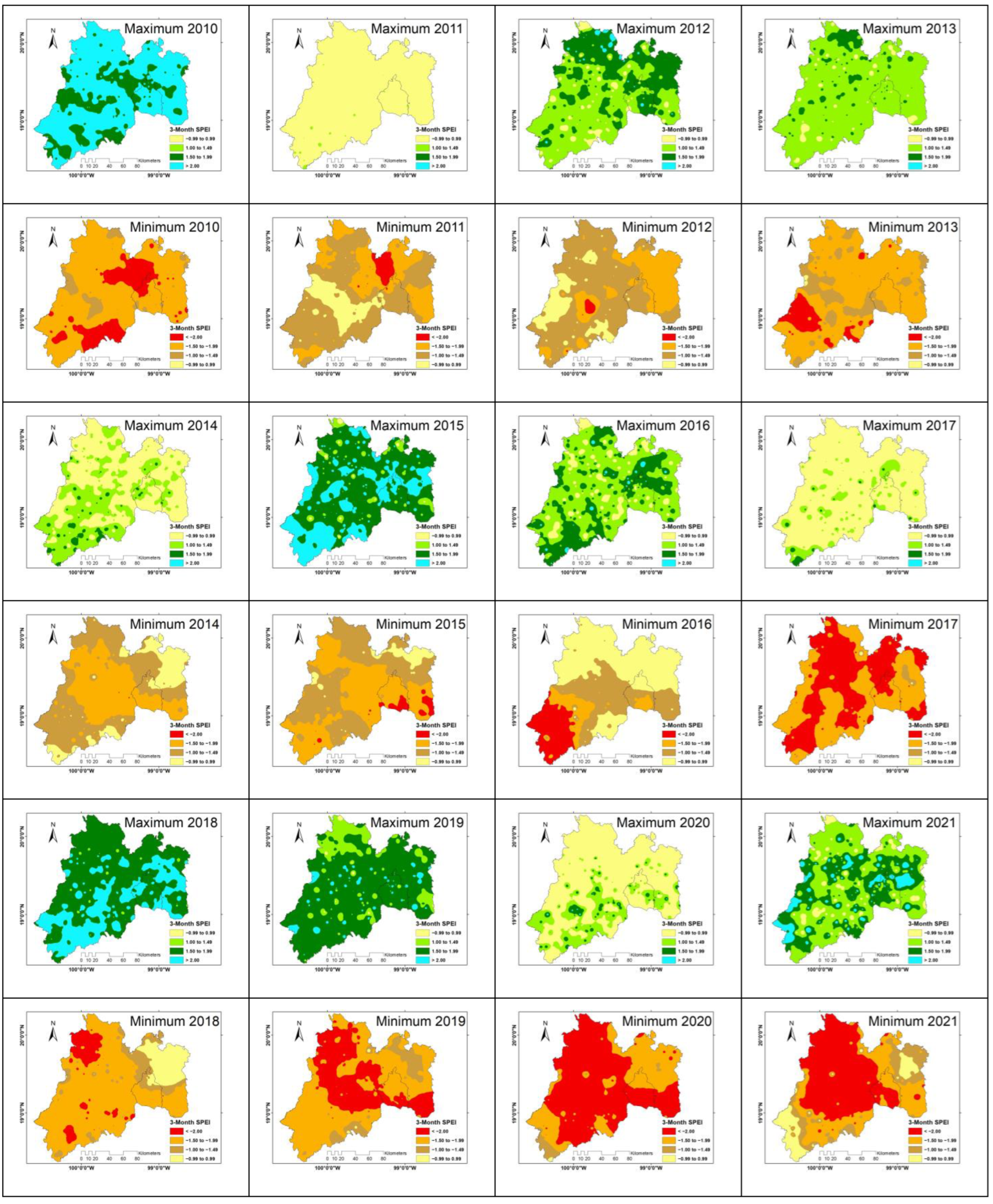
2.9.3. Standardized Precipitation Evapotranspiration Index (SPEI)

SPEI has certain similarities to SPI, except for the subtraction of evapotranspiration. In the SPEI calculation, we need the monthly water balance, which is based on the difference between rainfall and potential evapotranspiration (PET) [54], so that we can make a comparison of drought severity over time and space, as it can be calculated in a wide range of climates. Furthermore, Keyantash and Dracup [55] indicated that drought indices should be statistically robust and easy to calculate and have a clear and understandable calculation procedure.
For the calculation of the SPEI, the water balance equation (Di = Pi − ETo) is used. It calculates for several time scales (k) (i.e., for one month, two months, three months, etc.). For example, to obtain the value for SPEI of a time scale of 6 months, a time series is first created by adding the D values from five months ago to the current month.
For the original calculation of the SPEI, it was recommended to use the Thornthwaite equation for the estimation of ETo [44]. This equation only requires the mean daily temperature and the latitude of the site and was used due to limited data availability. However, other alternative equations can be used. The more robust FAO-56 Penman–Monteith equation [46] is recommended if data (relative humidity, temperature, wind speed, and solar radiation) are available, but when there is a lack of data required, the Hargreaves equation (first option) or the Thornthwaite equation (second option) are recommended. Differences between the SPEI series calculated using the different equations to estimate ETo can be significant in some regions of the world. In general, these differences were greater in semi-arid areas and smaller in humid regions [56]. In this work, the SPEI calculation was performed in the RStudio® program [57] using the SPEI.R package version 1.8.1, developed by Beguería and Vicente [56], at time scales of 1, 3, 6, 9, 12, and 24 months, with monthly meteorology data like precipitation, minimum and maximum temperatures, and latitude of the study point analyzed, and the Hargreaves method was selected for the calculation of evapotranspiration.
The values obtained were analyzed based on the SPEI classification and categories [12], Table 1. With this information, a temporal analysis was carried out, with the aim of understanding the evolution of droughts, identifying periods of moderate, severe, and extreme drought and defining their intensity, duration, and approximate start and end dates.

3. Results

Climatol was used to analyze 381 weather stations (Figure 2), focusing on temperature and precipitation data. The Standard Normal Homogeneity Test (SNHT) results for maximum and minimum temperatures were lower, suggesting that these datasets exhibit greater homogeneity over time, with less evidence of breakpoints or abrupt changes. In contrast, precipitation data showed a higher SNHT, indicating potential inhomogeneities due to factors such as station relocations, instrument changes, or climatic shifts.
Similarly, the Root Mean Square Error (RMSE) values for maximum and minimum temperatures were higher, reflecting poorer model accuracy. This suggests a greater discrepancy between predicted and observed values, indicating that the model’s temperature estimations may be less reliable. Conversely, precipitation data exhibited a lower RMSE, implying better model accuracy, with predictions aligning more closely with actual observations. This suggests that the model performed more effectively in reconstructing precipitation patterns than temperature trends.
The trend test found that most of the monthly precipitation data were 71.13%, with a non-significant increasing trend, and 28.87% with a non-significant decreasing trend of the total precipitation values. For the maximum temperature, it was found that 87.93% were valued with a significant increasing trend, 10.50% with a non-significant increasing trend, and 1.57% with a non-significant decreasing trend. The monthly minimum temperature had a 67.98% significant increasing trend, 27.56% non-significant increasing trend, and 4.46% non-significant decreasing trend. The tests performed detected whether the series has no persistence or trend, changes in the mean, or does not fluctuate too much. The results of these tests are presented with TSC for a significant increasing trend, TNSC for a non-significant increasing trend, TNSD for a non-significant decreasing trend, and TSD for a significant decreasing trend. The variables analyzed were precipitation, maximum temperature, and minimum temperature. A significant change in the mean is evidence of some impact by an external phenomenon, whether natural or man-made (Figure 3).
Taking this into account, the drought analysis was continued by calculating SPEI of the area with the meteorological records previously analyzed statistically. In general, the analysis of the SPEI values was carried out for the different time scales of 1, 3, 6, 9, 12, and 24 months in a period of 42 years, from 1981 to 2023, for the maximum and minimum values.
An analysis was carried out on the 3-month SPEI drought index from 2010 to 2023, which refers to the average accumulated precipitation in a 3-month period and is compared with the historical average precipitation in that same period. Positive SPEI values indicate a surplus of water content, that is, the land is receiving more water than it loses through evaporation. Negative values indicate a precipitation deficit, that is, the land is receiving less water than it loses through evaporation (Figure 4).
The 3-month SPEI drought index is a useful indicator to assess the severity of droughts in different regions and time scales, considering evaporation and accumulated precipitation over a 3-month period.
The information obtained through the maps of maximum and minimum values of SPEI acquired shows the evolution from the beginning in the year 2010, where the maximum values in most of the area are classified as “Extremely humid” and “Very humid”, while the minimum values are mostly considered “Extremely dry”, “Very dry”, and “Moderately dry”. Such maximum humidity obtains similar values only for the years 2015 and 2018. The rest of the years present a range of “Very humid” and “Moderately humid” in the years 2012, 2013, 2016, 2019, 2021, and 2023, with very few areas considered to be “Extremely humid”.
Although the maximum values (Figure 4) have a certain cycle where they tend to have values like 2010, the minimum values through the 14 years analyzed have a growth in negative values representing an “Extremely dry” category, which had a negative trend, with the years 2010, 2017, 2019, 2020, 2021, and 2023 being the most severe years with drought values, leaving the years like 2011, 2014, 2017, 2020, and 2022, where the humidity did not obtain values to be sufficiently humid in area and value, and having the lower values considered to be “Extremely dry” to be present in most of the area.
Figure 5 shows the severity of 6-month droughts for the years 2016 to 2023, with the drought being most severe in the western part of the State of Mexico, where the capital of the State of Mexico, Toluca, and the Cutzamala system that supplies drinking water to Mexico City are located (Figure 6). A three-month drought index should trigger a drought management program, but a six-month drought index is a cause for greater concern because a longer drought begins to affect aquifer recharge. The driest years were 2019, 2021, and 2023.
Figure 6 shows the comparison of the 6-month SPEI indices, 1981–2023, for two stations located in the west and east of the State of Mexico; note that since 2015, droughts measured through negative value indices are more severe in the western part of the State of Mexico, where the capital Toluca and the Cutzamala system that supplies water to Mexico City are located. Analyzing the INEGI reports on land use for the years 2009 and 2018 for the State of Mexico, the areas with human settlements, including large cities, have increased by 62% [34]. Likewise, the bare soil surface has tripled, and the agricultural area has decreased by 0.6% (61,500 ha). From 2009 to 2018, 2600 hectares of forests have been lost.

4. Discussion

Droughts are natural phenomena that affect different economic, natural resources, and social sectors. The focus of this study was the analysis of the time and space of the droughts presented in a lapse of 42 years in the State of Mexico and Mexico City (Figure 6). However, to obtain an adequate analysis of the droughts, it is optimal to have a series of abundant meteorological data. In regions like Mexico, the lack of data poses a significant challenge that must be addressed by leveraging new technologies, such as satellite observations calibrated with ground-based station measurements.
When analyzing the CHIRPS and DAYMET data used, a good correlation was found with a meteorological station. In our case, precipitation data had a non-significant trend, but temperature had a significant increasing trend. This trend was reflected in the central (Mexico City) and northern zones where human activity has increased.
The SPEI values considered moderately dry were presented in periods of an average of 5 years before having years considered wet. This behavior was increasing where the longest drought identified began in 1998 and ended in 2014, concentrating the affectation to the west of Mexico City and the central zone of the State of Mexico. A comparison of SPI with SPEI in other studies found that the performance of SPEI is better when considering the temperature values that influence evapotranspiration, which leads to possible drought conditions. Sometimes, detecting droughts solely based on precipitation data, as performed with the SPI, is not sufficient [20,21]. In the study area, an increase in temperature was detected, highlighting the need for an index such as SPEI [58,59]. Previous studies conducted in Mexico [22,23] have shown that SPEI is more effective in detecting drought conditions, as indicated by lower index values.
The areas most affected by drought include key surface water supply systems for Mexico City, particularly in the western part of the study region. Additionally, some of these areas serve as important aquifer recharge zones, making them highly vulnerable to water shortages.

5. Conclusions

Meteorological databases like CHIRPS and DAYMET are a solution for the lack of information in many regions in developing countries like Mexico. It is information analyzed with Climatol from the 381 stations and their values of maximum and minimum temperatures which had a low SNHT and a high RMSE, which means that the stations had no break points but large deviations, which suggests a local climatic influence or poor model estimation. For the precipitation, the values analyzed are from stations with detected breaks but still accurate predictions, as well as from high-quality stations.
The Mann–Kendall statistical test provided evidence that in the period analyzed, there is an increased trend in both minimum and maximum temperatures over the analyzed period. This trend may be a consequence of human activities and may also be the product of a sudden natural process. This increase in temperature was reflected in the SPEI value for the region analyzed. Because of the rise in temperatures, the recorded droughts increase in maximum intensity, total magnitude, and duration. On the contrary, the wet periods will show the opposite behavior.
The main findings on this study are that between the period of 1981–1985, 1988–1991, and 1998–2014, there were droughts considered as moderately dry, but the one in 1998 was the longest, which had short periods of three years of recovery in 2004 and 2008 with values considered close to normal, most of which were categorized as moderately dry and very dry.
In the last 14 years for a 3-month analysis, it was possible to see that the years with the highest wet values were 2010, 2015, and 2018, with the year 2021 and 2023 having a moderate recovery of wet; however, the years with the most severe drought were 2017, 2019, 2020, 2021, and 2023 because of the increase in temperatures.
The increase in frequency of drought events has a pattern that presents itself every five years, but in recent years, it has increased in intensity, as well as the amount of area that has been categorized as extremely dry and very dry.

Author Contributions

Conceptualization, M.C.-C. and L.I.-C.; methodology, M.C.-C.; software, M.C.-C.; validation, L.I.-C., R.A.-R. and G.A.-G.; formal analysis, M.C.-C.; investigation, M.C.-C.; resources, M.C.-C.; data curation, R.A.-R.; writing—original draft preparation, M.C.-C.; writing—review and editing, L.I.-C.; visualization, G.A.-G.; supervision, L.I.-C.; project administration, L.I.-C.; funding acquisition, G.A.-G. All authors have read and agreed to the published version of the manuscript.

Funding

This research was funded by the National Council of Humanities, Science and Technology, CONAHCYT, of Mexico (No. 320262).

Institutional Review Board Statement

Not applicable.

Informed Consent Statement

Not applicable.

Data Availability Statement

The data presented in this study are available upon request from the corresponding author. The data are not publicly available due to privacy.

Acknowledgments

To the National Council of Humanities, Science and Technology, CONAHCYT, of Mexico for the financial support provided in the form of a postgraduate maintenance scholarship for the development of this research.

Conflicts of Interest

The authors declare no conflicts of interest.

References

  1. Smakhtin, V.U.; Schipper, E.L.F. Droughts: The impact of semantics and perceptions. Water Policy 2008, 10, 131. [Google Scholar] [CrossRef]
  2. Stahl, K.; Kohn, I.; Blauhut, V.; Urquijo, J.; de Stefano, L.; Acácio, V.; Dias, S.; Stagge, J.H.; Tallaksen, L.M.; Kampragou, E.; et al. Impacts of European drought events: Insights from an international database of text-based reports. Nat. Hazards Earth Syst. Sci. 2016, 16, 801–819. [Google Scholar] [CrossRef]
  3. Dai, A. Drought under global warming: A review. WIREs Clim Chang. 2011, 2, 45–65. [Google Scholar] [CrossRef]
  4. Zhang, Q.; Yao, Y.B.; Li, Y.H.; Huang, J.P.; Ma, Z.G.; Wang, Z.L.; Wang, S.P.; Wang, Y.; Zhang, Y. Progress and prospect on the study of causes and variation regularity of droughts in China. Acta Meteorol. Sin. 2020, 78, 500–521. [Google Scholar] [CrossRef]
  5. Meyer, S.J.; Hubbard, K.G.; Wilhite, D.A. A crop-specific drought index for corn: I. Model development and validation. Agron. J. 1993, 85, 388–395. [Google Scholar] [CrossRef]
  6. Calviño, P.A.; Andrade, F.H.; Sadras, V.O. Maize yield as affected by water availability, soil depth, and crop management. Agron. J. 2003, 95, 275–281. [Google Scholar] [CrossRef]
  7. Hunt, E.D.; Svoboda, M.; Wardlow, B.; Hubbard, K.; Hayes, M.; Arkebauer, T. Monitoring the effects of rapid onset of drought on non-irrigated maize with agronomic data and climate-based drought indices. Agric. For. Meteorol. 2014, 191, 1–11. [Google Scholar] [CrossRef]
  8. Real-Rangel, R.A.; Pedrozo-Acuña, A.; Breña-Naranjo, J.A.; Alcocer-Yamanaka, V.H. Monitorización de sequías en México a través del índice estandarizado multivariado de sequía. In Proceedings of the XXIV Congreso Nacional de Hidráulica, Acapulco, Guerrero, México, 22–25 March 2017. [Google Scholar]
  9. Wilhite, D.A. Drought as a natural hazard: Concepts and definitions. In Drought: A Global Assessment; Wilhite, D., Ed.; Routledge: London, UK, 2000; Volume 1, pp. 3–18. [Google Scholar]
  10. Burton, I.; Kates, R.W.; White, G.F. The Environment as Hazard; Oxford University Press: New York, NY, USA, 1978; 240p. [Google Scholar]
  11. Sun, Y.; Chen, X.; Yu, Y.; Qian, J.; Wang, M.; Huang, S.; Xing, X.; Song, S.; Sun, X. Spatiotemporal Characteristics of Drought in Central Asia from 1981 to 2020. Atmosphere 2022, 13, 1496. [Google Scholar] [CrossRef]
  12. McKee, T.B.; Doesken, N.J.; Kleist, J. The relationship of drought frequency and duration to time scales. In Proceedings of the 8th Conference on Applied Climatology, Anaheim, CA, USA, 17–22 January 1993; American Meteorological Society: Boston, MA, USA, 1993; pp. 179–183. [Google Scholar]
  13. Guttman, N.B. Comparing the Palmer drought index and the Standardized Precipitation Index. J. Am. Water Resour. Assoc. 1998, 34, 113–121. [Google Scholar] [CrossRef]
  14. WMO. Drought Monitoring and Early Warning: Concepts, Progress and Future Challenges; WMO: Geneva, Switzerland, 2006. [Google Scholar]
  15. Hayes, M.; Svoboda, M.; Wall, N.; Widhalm, M. The Lincoln declaration on drought indices: Universal meteorological drought index recommended. Bull. Am. Meteorol. Soc. 2011, 92, 485–488. [Google Scholar] [CrossRef]
  16. Hao, Z.; AghaKouchak, A.; Phillips, T.J. Changes in concurrent monthly precipitation and temperature extremes. Environ. Res. Lett. 2013, 8, 034014. [Google Scholar] [CrossRef]
  17. Ren, L.; Zhou, T.; Zhang, W. Attribution of the record-breaking heat event over Northeast Asia in summer 2018: The role of circulation. Environ. Res. Lett. 2020, 15, 054018. [Google Scholar] [CrossRef]
  18. Wang, L.Y.; Yuan, X. Two types of flash drought and their connections with seasonal drought. Adv. Atmos. Sci. 2018, 35, 1478–1490. [Google Scholar] [CrossRef]
  19. Yuan, X.; Wang, Y.M.; Zhang, M.; Wang, L.Y. A few thoughts on the study of flash drought (in Chinese). Trans. Atmos. Sci. 2020, 43, 1086–1095. [Google Scholar]
  20. Monitor de Sequía en México. Servicio Meteorológico Nacional. 2024. Available online: https://smn.conagua.gob.mx/es/climatologia/monitor-de-sequia/monitor-de-sequia-en-mexico (accessed on 30 October 2024).
  21. Vicente-Serrano, S.M.; Beguería, S.; López-Moreno, J.I. A multi-scalar drought index sensitive to global warming: The standardized precipitation evapotranspiration index—SPEI. J. Clim. 2010, 23, 1696–1718. [Google Scholar] [CrossRef]
  22. Castillo-Castillo, M.; Ibáñez-Castillo, L.; Valdés, J.B.; Arteaga-Ramirez, R. Análisis de sequías meteorológicas en la cuenca del río Fuerte, México. Tecnol. Y Cienc. Del Agua 2017, 8, 35–52. [Google Scholar] [CrossRef]
  23. Hernández-Vásquez, C.C.; Ibáñez-Castillo, L.A.; Gómez-Díaz, J.D.; Arteaga-Ramírez, R. Analysis of meteorological droughts in the Sonora River basin Mexico. Atmósfera 2022, 35, 467–482. [Google Scholar] [CrossRef]
  24. Dinku, T.; Funk, C.; Peterson, P.; Maidment, R.; Tadesse, T.; Gadain, H.; Ceccato, P. Validation of the CHIRPS satellite rainfall estimates over eastern Africa. Q. J. R. Meteorol. Soc. 2018, 144 (Suppl. 1), 292–312. [Google Scholar] [CrossRef]
  25. Funk, C.; Peterson, P.; Landsfeld, M.; Pedreros, D.; Verdin, J.; Shukla, S.; Husak, G.; Rowland, J.; Harrison, L.; Hoell, A.; et al. The climate hazards group infrared precipitation with stations—A new environmental record for monitoring extremes. Sci. Data 2015, 2, 150066. [Google Scholar] [CrossRef]
  26. CONAGUA (Comisión Nacional del Agua). Programa de medidas preventivas y de mitigación de la sequía. In Consejo de Cuenca ríos Fuerte y Sinaloa; Comisión Nacional del Agua, Secretaría de Medio Ambiente y Recursos Naturales: Ciudad de México, Mexico, 2014; p. 262. [Google Scholar]
  27. INEGI Monografías. 2024. Available online: https://cuentame.inegi.org.mx/monografias/ (accessed on 4 November 2024).
  28. INEGI (Instituto Nacional de Estadística, Geografía e Informática). 2020 Censo de Población y Vivienda. México. 2023. Available online: https://www.inegi.org.mx/datosabiertos/ (accessed on 10 September 2023).
  29. Guijarro, J.A. Climatol: A software tool for the validation and analysis of climate data. Environ. Model. Softw. 2018, 105, 1–10. [Google Scholar]
  30. Kuya, E.K.; Gjelten, H.M.; Tveito, O.E. Homogenization of Norwegian monthly precipitation series for the period 1961–2018. Adv. Sci. Res. 2022, 19, 73–80. [Google Scholar] [CrossRef]
  31. Tudorache, G. Analysing the homogeneity of air temperature, relative air humidity, precipitation and wind data series using ‘Climatol’ and meteorological metadata. Aerul Şi Apa Compon. Ale Mediului. 2017, 2017, 50–57. [Google Scholar] [CrossRef]
  32. HydroGeoLogic, Inc. -OU-1 Informe Anual de Monitoreo de Aguas Subterráneas de 2004; HydroGeoLogic, Inc.: Antiguo Fort Ord, CA, USA, 2005. [Google Scholar]
  33. Kendall, M.G. Rank Correlation Methods; Charles Griffin: London, UK, 1975; p. 120. [Google Scholar]
  34. Mann, H.B. Nonparametric tests against trend. Econometrica 1945, 13, 245–259. [Google Scholar] [CrossRef]
  35. Yu, J.-Y.; Kao, H.-Y. Decadal changes of El Niño persistence barrier in SST and ocean heat content indices: 1958–2001. Geophys. Res. Lett. 2007, 112, D13106. [Google Scholar] [CrossRef]
  36. Silva, D.G. Evolução Paleoambiental dos Depósitos de Tanques em Fazenda Nova, Município de Brejo da Madre de Deus—Pernambuco. Master’s Thesis, UFPE, Recife, Brazil, 2007. [Google Scholar]
  37. Climate Engine. Desert Research Institute and University of California, Merced. version 2.1. 2024. Available online: http://climateengine.org (accessed on 7 April 2024).
  38. Funk, C.; Michaelsen, J.; Marshall, M. Mapping recent decadal climate variations in precipitation and temperature across Eastern Africa and the Sahel. In Remote Sensing of Drought—Innovative Monitoring Approaches; Wardlow, B., Anderson, M., Verdin, J., Eds.; Taylor and Francis: London, UK, 2012; pp. 331–357. [Google Scholar]
  39. Funk, C.; Verdin, J.; Michaelsen, J.; Peterson, P.; Pedreros, D.; Husak, G. A global satellite assisted precipitation climatology. Earth Syst. Sci. Data Discuss. 2015, 7, 1–13. [Google Scholar] [CrossRef]
  40. Funk, C.; Peterson, P.; Landsfeld, M.; Pedreros, D.; Verdin, J.; Rowland, J.; Romero, B.; Husak, G.; Michaelsen, J.; Verdin, A. A quasi-global precipitation time series for drought monitoring. U.S. Geol. Surv. Data Ser. 2014, 832, 4. [Google Scholar] [CrossRef]
  41. Maidment, R.; Grimes, D.; Black, E.; Tarnavsky, E.; Young, M.; Greatrex, H.; Allan, R.P.; Stein, T.; Nkonde, E.; Senkunda, S.; et al. A new, long-term daily satellite-based rainfall dataset for operational monitoring in Africa. Sci. Data 2017, 4, 170063. [Google Scholar] [CrossRef]
  42. Thornton, M.M.; Shrestha, R.; Wei, Y.; Thornton, P.E.; Kao, S.-C.; Wilson, B.E. Daymet: Daily Surface Weather Data on a 1-km Grid for North America, Version 4 R1; ORNL DAAC: Oak Ridge, TN, USA, 2022. [Google Scholar] [CrossRef]
  43. McMahon, T.A.; Peel, M.C.; Lowe, L.; Srikanthan, R.; McVicar, T.R. Estimating actual, potential, reference crop and pan evaporation using standard meteorological data: A pragmatic synthesis. Hydrol. Earth Syst. Sci. 2013, 17, 1331–1363. [Google Scholar] [CrossRef]
  44. Thornthwaite, C.W. An approach toward a rational classification of climate. Geogr. Rev. 1948, 38, 55–94. [Google Scholar] [CrossRef]
  45. Hargreaves, G.H.; Samani, Z.A. Reference Crop Evapotranspiration from Ambient Air Temperature; American Society of Agricultural Engineers: St. Joseph, MI, USA, 1985; pp. 96–99. [Google Scholar]
  46. Allen, R.; Pereira, L.; Raes, D.; Smith, M. Crop evapotranspiration. In FAO Irrigation and Drainage Paper 56; FAO: Rome, Italy, 1998; Volume 10. [Google Scholar]
  47. Priestley, C.H.B.; Taylor, R.J. On the assessment of surface heat flux and evaporation using large-scale parameters. Mon. Weather. Rev. 1972, 100, 81–92. [Google Scholar] [CrossRef]
  48. Jensen, M.E. Consumptive Use of Water and Irrigation Water Requirements; American Society of Civil Engineers: New York, NY, USA, 1973. [Google Scholar]
  49. Amatya, D.; Skaggs, R.; Gregory, J. Comparison of methods for estimating REF-ET. J. Irrig. Drain. Div. ASCE 1995, 121, 427–435. [Google Scholar] [CrossRef]
  50. WFD; Hadley Centre for Climate Prediction and Research/Met Office/Ministry of Defence/United Kingdom. WATer and global CHange (WATCH) Forcing Data (WFD)—20th Century. In Research Data Archive at the National Center for Atmospheric Research, Computational and Information Systems Laboratory; NCAR: Boulder, CO, USA, 2018. [Google Scholar] [CrossRef]
  51. NIDIS, National Integrated Drought Information System, US Government. Drought Basics. 2025. Available online: https://www.drought.gov/what-is-drought/drought-basics (accessed on 3 February 2025).
  52. Wells, N.; Goddard, S.; Hayes, M.J. A self-calibrating Palmer Drought Severity Index. J. Clim. 2004, 17, 2335–2351. [Google Scholar] [CrossRef]
  53. Moazzam, M.F.U.; Rahman, G.; Munawar, S.; Farid, N.; Lee, B.G. Spatiotemporal Rainfall Variability and Drought Assessment during Past Five Decades in South Korea Using SPI and SPEI. Atmosphere 2022, 13, 292. [Google Scholar] [CrossRef]
  54. Vicente-Serrano, S.M.; National Center for Atmospheric Research Staff. (Eds.) The Climate Data Guide: Standardized Precipitation Evapotranspiration Index (SPEI). 2024. Available online: https://climatedataguide.ucar.edu/climate-data/standardized-precipitation-evapotranspiration-index-spei (accessed on 19 April 2023).
  55. Keyantash, J.; Dracup, J. The quantification of drought: An evaluation of drought indices. Bull. Am. Meteorol. Soc. 2002, 83, 1167–1180. [Google Scholar] [CrossRef]
  56. Beguería, S.; Vicente, S.; Calculation of the Standardized Precipitation-Evapotranspiration Index. Package SPEI.R for R or RStudio Program. 2014. Available online: https://cran.r-project.org/web/packages/SPEI/index.html (accessed on 14 May 2023).
  57. RStudio, Inc. RStudio® Version 2023.03.1; RStudio, Inc.: Boston, MA, USA, 2023. [Google Scholar]
  58. Sung, J.H.; Park, J.; Jeon, J.-J.; Seo, S.B. Assessment of inter-model variability in meteorological drought characteristics using CMIP5 GCMs over South Korea. KSCE J. Civ. Eng. 2020, 24, 2824–2834. [Google Scholar] [CrossRef]
  59. Jang, D. Assessment of meteorological drought indices in Korea using RCP 8.5 scenario. Water 2018, 10, 283. [Google Scholar] [CrossRef]
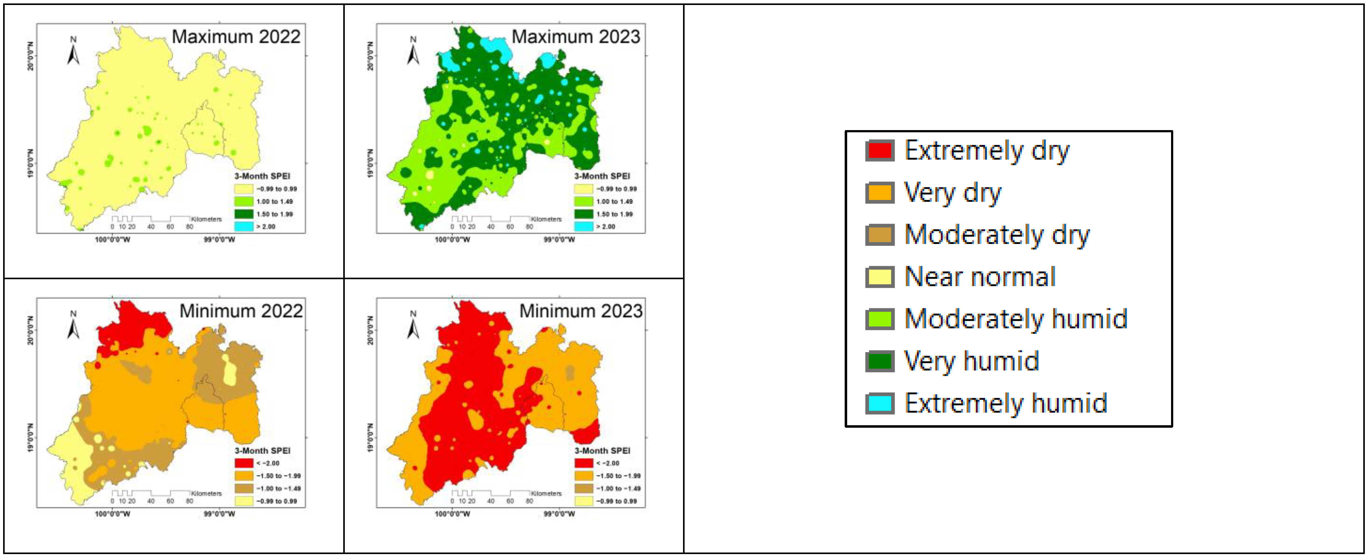
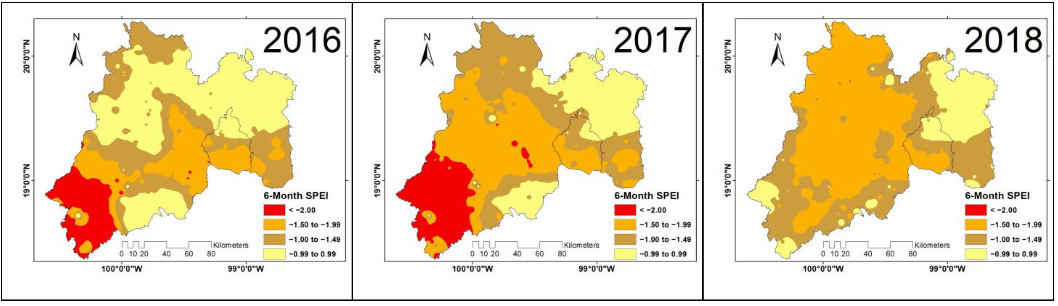
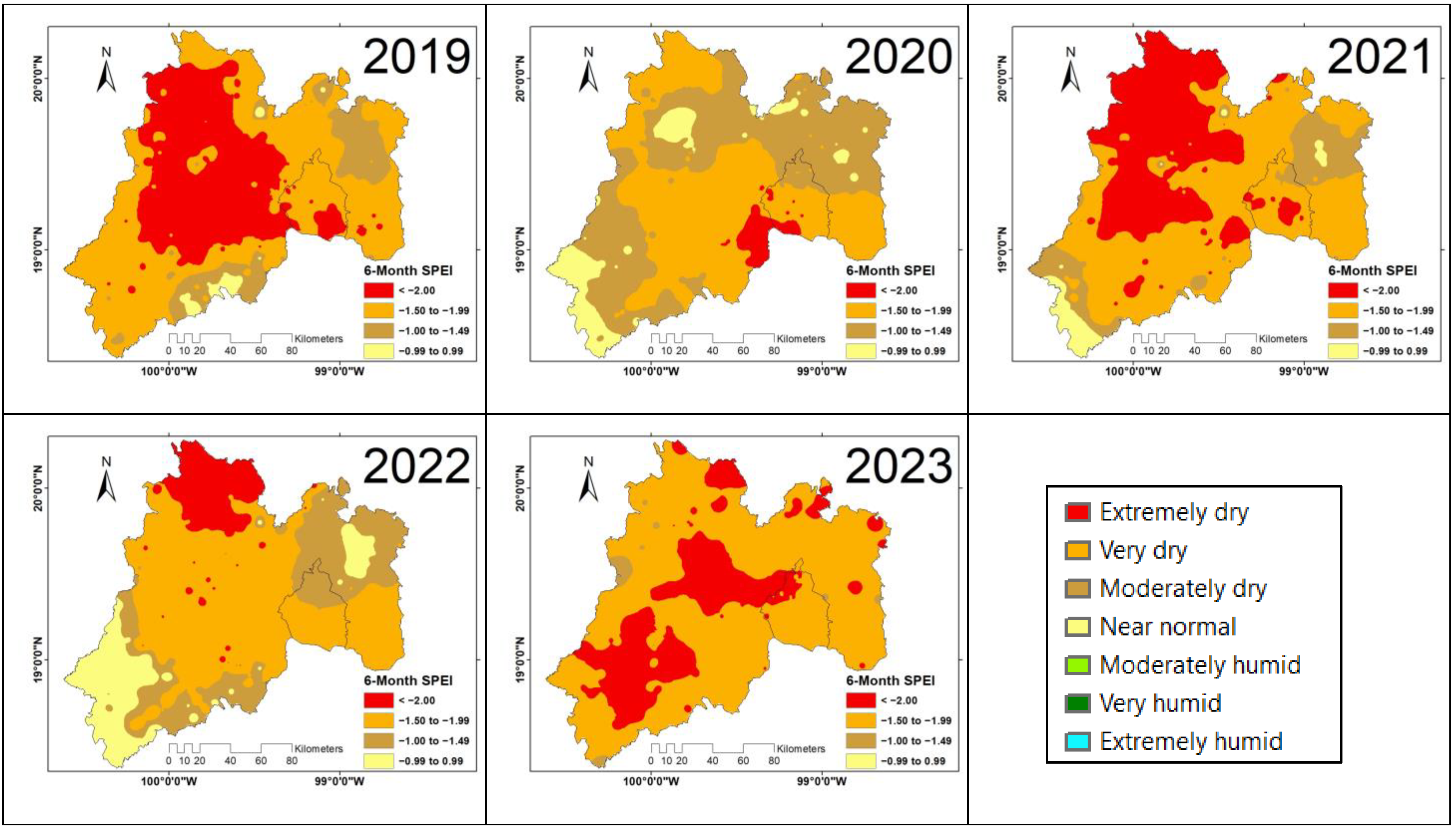
Figure 1. Location of the State of Mexico, Mexico City, and the 381 weather stations operated by the SMN.
Atmosphere 16 00202 g001
Figure 2. Quality, singularity, and location of the 381 stations obtained from Climatol each different symbols represents a different station.
Atmosphere 16 00202 g002
Figure 3. Trends in the variables analyzed in the study area (TSC = significant increasing trend; TSD = significant decreasing trend; TNSC = non-significant increasing trend; TNSD = non-significant decreasing trend).
Atmosphere 16 00202 g003
Figure 4. Spatial distribution of maximum and minimum SPEI values calculated for a 3-month time scale (2010–2023).
Atmosphere 16 00202 g004aAtmosphere 16 00202 g004b
Figure 5. The most severe six-month drought indices in Mexico City and the State of Mexico from 2016 to 2023.
Atmosphere 16 00202 g005aAtmosphere 16 00202 g005b
Figure 6. Temporal variation of the 6-month SPEI index comparing a station in the west (Valle de Bravo) with a station in the east (Texcoco) of the State of Mexico.
Atmosphere 16 00202 g006
Table 1. SPEI categories and classification [12].
Index ValueCategory
>2.00Extremely humid
1.50 to 1.99Very humid
1.00 to 1.49Moderately humid
−0.99 to 0.99Near normal
−1.00 to −1.49Moderately dry
−1.50 to −1.99Very dry
<−2.00Extremely dry
Disclaimer/Publisher’s Note: The statements, opinions and data contained in all publications are solely those of the individual author(s) and contributor(s) and not of MDPI and/or the editor(s). MDPI and/or the editor(s) disclaim responsibility for any injury to people or property resulting from any ideas, methods, instructions or products referred to in the content.

