


Towards Sustainable Shipping: Joint Optimization of Ship Speed and Bunkering Strategy Considering Ship Emissions


Abstract
:1. Introduction
2. Methods
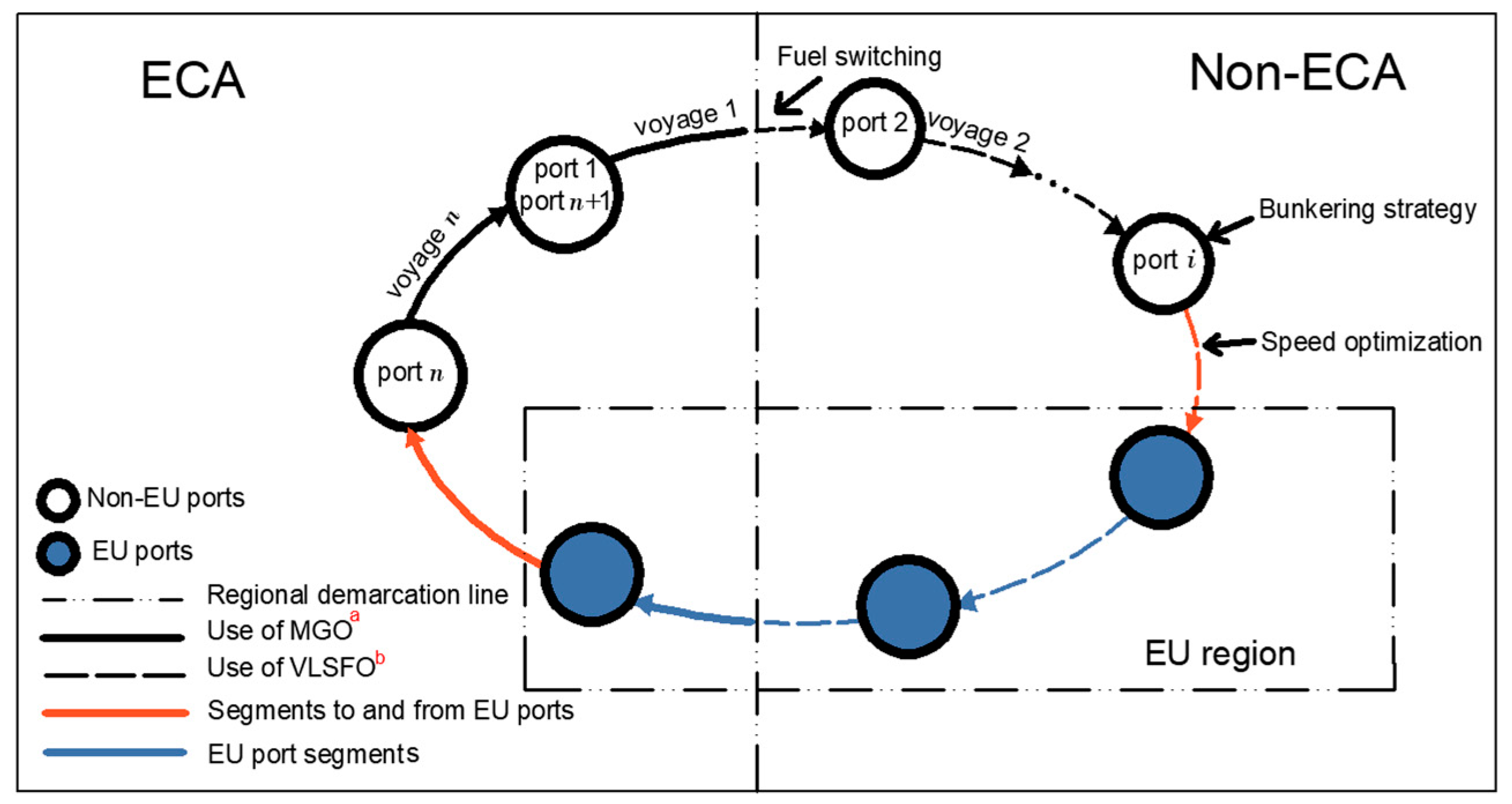
2.1. Problem Description and Assumptions
- (1)
- (2)
- (3)
- The fuel oil switching time is not considered, the port is free of congestion and ships do not have to queue or wait at the port [28].
- (4)
- The fuel consumption of boilers is not considered because it is low [29].
- (5)
- The vessel only refuels at the ports of call, and the fuel prices at port are known before the vessel departs. The frequency of the departures is weekly, and the total time for a round trip is a constant [18].
2.2. Model Formulation and Cost Analysis
2.2.1. Parameters and Variables
- (1)
- Sets and parameters
- (2)
- Variables
2.2.2. Operating Cost Analysis
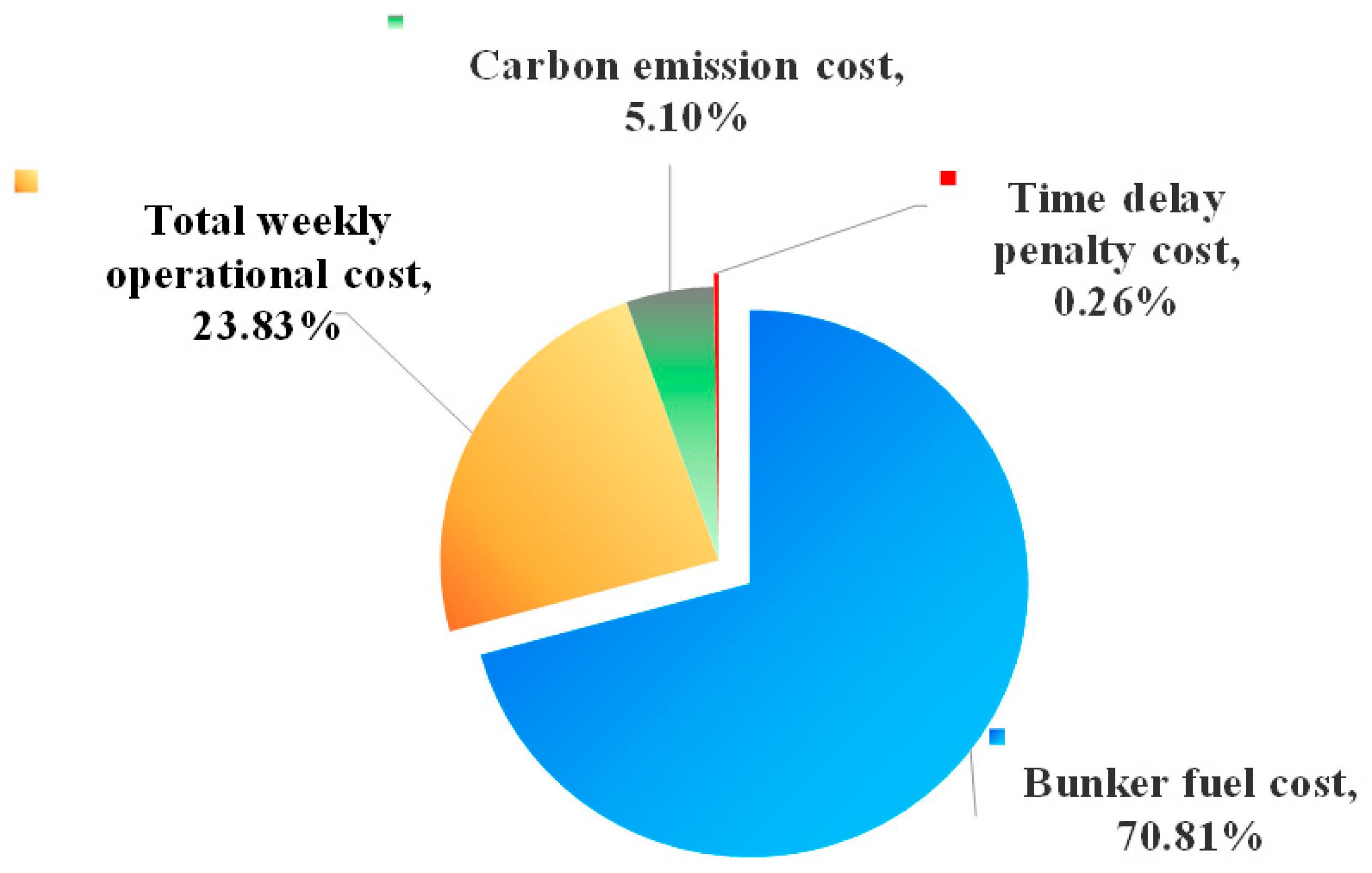
- The total weekly operational cost, CZE
- 2.
- Time delay penalty cost, CT
- 3.
- Carbon emission cost, CA
- (1)
- Fuel consumption
- (2)
- Carbon emissions
- (3)
- Carbon emission cost, CA
- 4.
- Bunker fuel cost, CF
2.2.3. Model Formulation
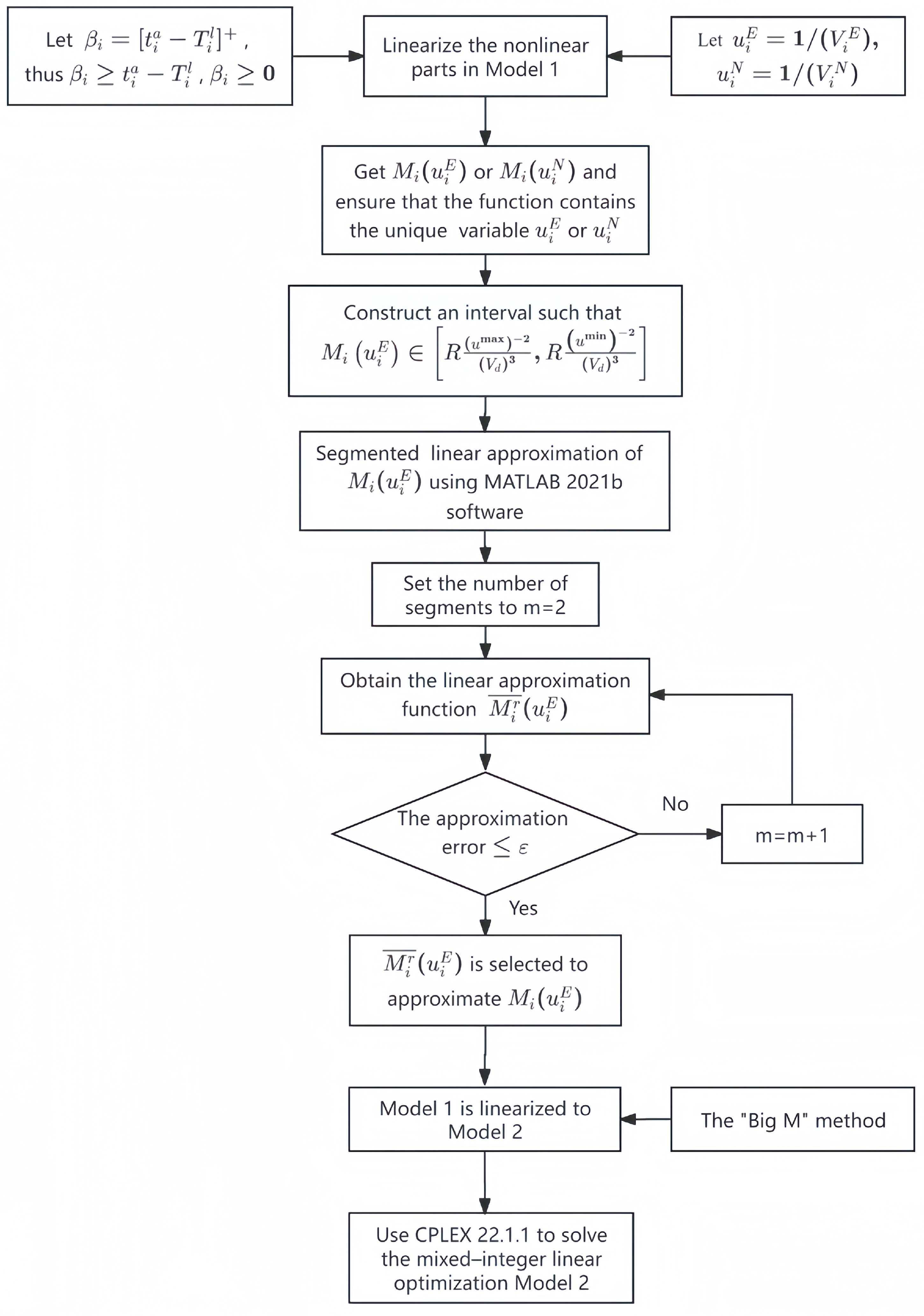
2.3. Model Transformation
3. Results
4. Discussion
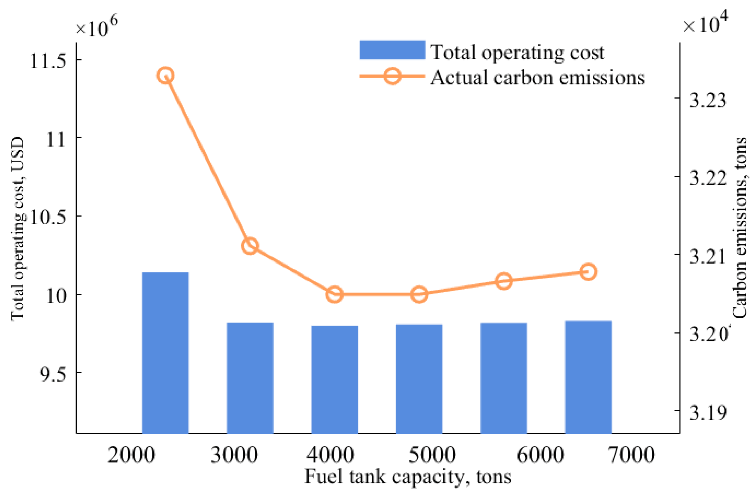
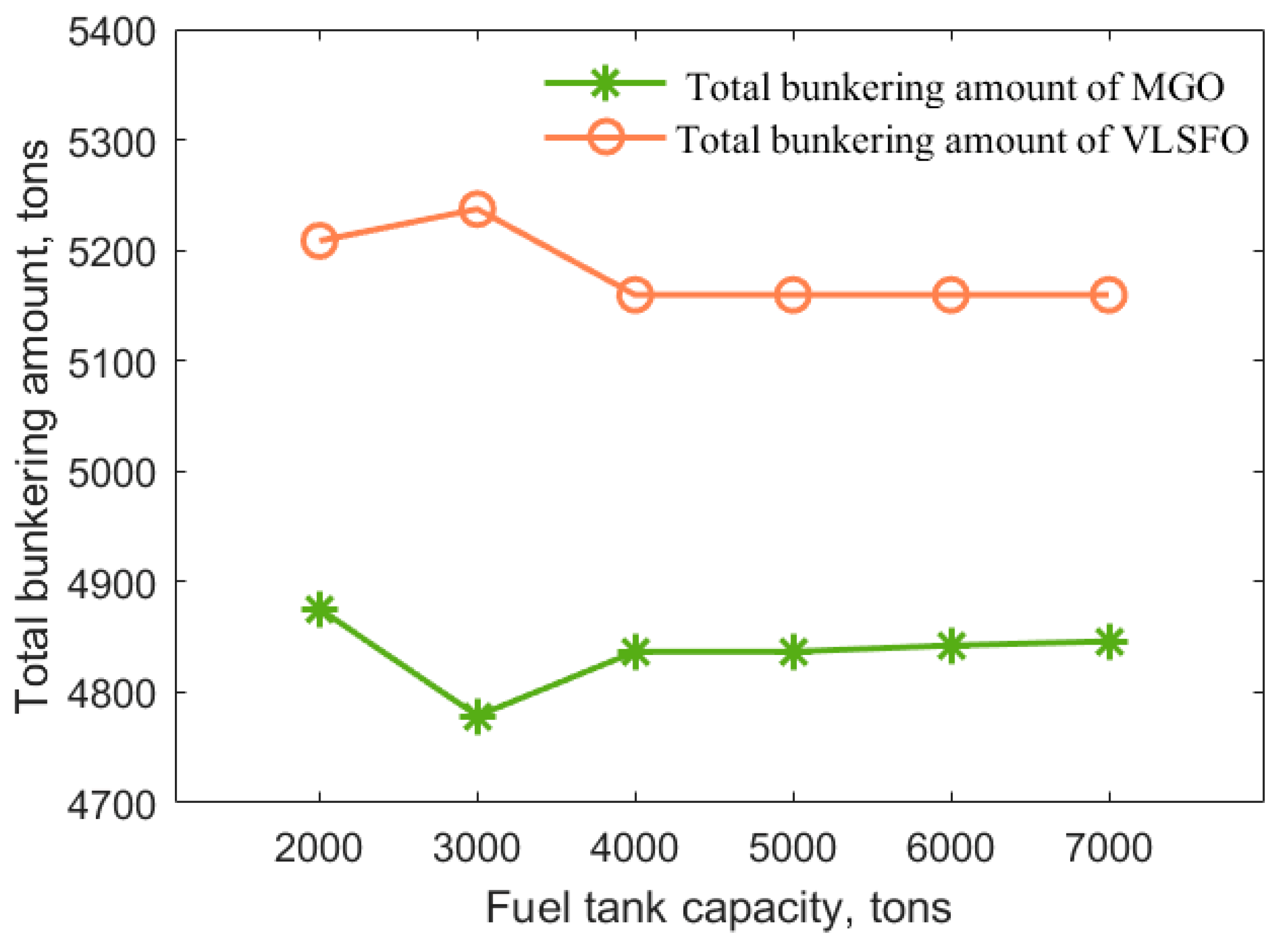
4.1. Effect of Fuel Tank Capacity
4.2. Effect of Fuel Price Spread
5. Conclusions
Author Contributions
Funding
Institutional Review Board Statement
Informed Consent Statement
Data Availability Statement
Acknowledgments
Conflicts of Interest
References
- Alamoush, A.S.; Ölçer, A.I.; Ballini, F. Ports’ role in shipping decarbonisation: A common port incentive scheme for shipping Greenhouse Gas Emissions reduction. Clean. Logist. Supply Chai. 2022, 3, 100021. [Google Scholar] [CrossRef]
- Lee, J.; Chen, J.; Yip, T.L.; Lee, H. A Study on the forecast of fine dust emissions in the future according to the introduction of eco-friendly ships. Mar. Pollut. Bull. 2025, 212, 117507. [Google Scholar] [CrossRef]
- IMO. Further Shipping GHG Emission Reduction Measures Adopted. 17 June 2021. Available online: https://www.imo.org/en/MediaCentre/PressBriefings/pages/MEPC76.aspx (accessed on 21 January 2025).
- Hua, R.; Yin, J.; Wang, S.; Han, Y.; Wang, X. Speed optimization for maximizing the ship’s economic benefits considering the carbon intensity indicator (CII). Ocean Eng. 2024, 293, 116712. [Google Scholar] [CrossRef]
- IMO. Revised GHG Reduction Strategy for Global Shipping Adopted. 7 July 2023. Available online: https://www.imo.org/en/MediaCentre/PressBriefings/pages/Revised-GHG-reduction-strategy-for-global-shipping-adopted-.aspx (accessed on 29 March 2024).
- IMO. IMO 2020—Cleaner Shipping for Cleaner Air. 20 December 2019. Available online: https://www.imo.org/en/MediaCentre/PressBriefings/pages/34-IMO-2020-sulphur-limit-.aspx (accessed on 29 March 2024).
- MOT. Notice of the Ministry of Transport on the Implementation Plan for the Emission Control Areas for Atmospheric Pollutants from Ships. 30 November 2018. Available online: https://xxgk.mot.gov.cn/2020/xzgfxwj/202303/t20230316_3775697.html (accessed on 28 March 2024).
- Adland, R.; Fonnes, G.; Jia, H.; Lampe, O.D.; Strandenes, S.P. The impact of regional environmental regulations on empirical vessel speeds. Transp. Res. Part D 2017, 53, 37–49. [Google Scholar] [CrossRef]
- Zhong, H.; Guo, C.; Yip, T.L.; Gu, Y. Bi-perspective sulfur abatement options to mitigate coastal shipping ships emissions: A case study of Chinese coastal zone. Ocean Coast. Manag. 2021, 209, 105658. [Google Scholar] [CrossRef]
- Li, L.; Gao, S.; Yang, W.; Xiong, X. Ship’s response strategy to Emission Control Areas: From the perspective of sailing pattern optimization and evasion strategy selection. Transp. Res. Part E 2020, 133, 101835. [Google Scholar] [CrossRef]
- Jiang, L.; Hu, J. Fleet deployment optimization and emission reduction strategy selection under sulfur emission limits. J. Shanghai Marit. Univ. 2021, 42, 81–87. [Google Scholar]
- He, P.; Jin, J.G.; Pan, W.; Chen, J. Route, speed, and bunkering optimization for LNG-fueled tramp ship with alternative bunkering ports. Ocean Eng. 2024, 305, 117957. [Google Scholar] [CrossRef]
- Notteboom, T.E.; Vernimmen, B. The effect of high fuel costs on liner service configuration in container shipping. J. Transp. Geogr. 2009, 17, 325–337. [Google Scholar] [CrossRef]
- Adland, R.; Cariou, P.; Wolff, F.C. Optimal ship speed and the cubic law revisited: Empirical evidence from an oil tanker fleet. Transp. Res. Part E 2020, 140, 101972. [Google Scholar] [CrossRef]
- Zhen, L.; Hu, Z.; Yan, R.; Zhuge, D.; Wang, S. Route and speed optimization for liner ships under emission control policies. Transp. Res. Part C 2020, 110, 330–345. [Google Scholar] [CrossRef]
- Sheng, D.; Meng, Q.; Li, Z.-C. Optimal vessel speed and fleet size for industrial shipping services under the Emission Control Area regulation. Transp. Res. Part C 2019, 105, 37–53. [Google Scholar] [CrossRef]
- Zhao, S.; Duan, J.; Li, D.; Yang, H. Vessel scheduling and bunker management with speed deviations for liner shipping in the presence of collaborative agreements. IEEE Access 2022, 10, 107669–107684. [Google Scholar] [CrossRef]
- Lashgari, M.; Akbari, A.A.; Nasersarraf, S. A new model for simultaneously optimizing ship route, sailing speed, and fuel consumption in a shipping problem under different price scenarios. Appl. Ocean Res. 2021, 113, 102725. [Google Scholar] [CrossRef]
- Dulebenets, M.A. Green vessel scheduling in liner shipping: Modeling Carbon Dioxide emission costs in sea and at ports of call. Int. J. Transp. Sci. Technol. 2018, 7, 26–44. [Google Scholar] [CrossRef]
- Ma, W.; Han, Y.; Tang, H.; Ma, D.; Zheng, H.; Zhang, Y. Ship route planning based on intelligent mapping swarm optimization. Comput. Ind. Eng. 2023, 176, 108920. [Google Scholar] [CrossRef]
- Sun, L.; Wang, X.; Hu, Z.; Liu, W.; Ning, Z. Carbon reduction and cost control of container shipping in response to the European Union Emission Trading System. Environ. Sci. Pollut. Res. 2024, 31, 21172–21188. [Google Scholar] [CrossRef]
- Sun, L.; Wang, X.; Hu, Z.; Ning, Z. Carbon and cost accounting for liner shipping under the European Union Emission Trading System. Front. Mar. Sci. 2024, 11, 1291968. [Google Scholar] [CrossRef]
- IMO. Sulphur Oxides (SOx) and Particulate Matter (PM)—Regulation 14. 2020. Available online: https://www.imo.org/en/OurWork/Environment/Pages/Sulphur-oxides-(SOx)-%E2%80%93-Regulation-14.aspx (accessed on 6 July 2024).
- European Commission. Reducing Emissions from the Shipping Sector. 2023. Available online: https://climate.ec.europa.eu/eu-action/transport/reducing-emissions-shipping-sector_en (accessed on 1 April 2024).
- IMO. Resolution MEPC.376(80) (Adopted on 7 July 2023) Guidelines on Life Cycle GHG Intensity of Marine Fuels; MERC: London, UK, 2023; pp. 49–50. Available online: https://wwwcdn.imo.org/localresources/en/OurWork/Environment/Documents/annex/MEPC%2080/Annex%2014.pdf (accessed on 7 July 2024).
- Fan, L.; Gu, B.; Luo, M. A cost-benefit analysis of fuel-switching vs. hybrid scrubber installation: A container route through the Chinese SECA case. Transp. Policy 2020, 99, 336–344. [Google Scholar] [CrossRef]
- Doudnikoff, M.; Lacoste, R. Effect of a speed reduction of containerships in response to higher energy costs in Sulphur Emission Control Areas. Transp. Res. Part D 2014, 28, 51–61. [Google Scholar] [CrossRef]
- Ma, D.; Ma, W.; Jin, S.; Ma, X. Method for simultaneously optimizing ship route and speed with Emission Control Areas. Ocean Eng. 2020, 202, 107170. [Google Scholar] [CrossRef]
- Wang, Q.; Wang, J.; Qu, Y.; Yu, T. Assessing the impact of Covid-19 on air pollutant emissions from vessels in Lianyungang Port. Mar. Pollut. Bull. 2023, 194, 115313. [Google Scholar] [CrossRef]
- Joung, T.H.; Kang, S.G.; Lee, J.K.; Ahn, J. The IMO initial strategy for reducing Greenhouse Gas (GHG) emissions, and its follow-up actions towards 2050. J. Int. Marit. Saf. Environ. Aff. Shipp. 2020, 4, 1–7. [Google Scholar] [CrossRef]
- European Commission. Delivering the European Green Deal. 1 July 2021. Available online: https://commission.europa.eu/strategy-and-policy/priorities-2019-2024/european-green-deal/delivering-european-green-deal_en#making-transport-sustainable-for-all (accessed on 25 May 2024).
- European Commission. Scope of the EU Emissions Trading System. 22 May 2023. Available online: https://climate.ec.europa.eu/eu-action/eu-emissions-trading-system-eu-ets/scope-eu-emissions-trading-system_en (accessed on 29 March 2024).
- Wang, S.; Zhuge, D.; Zhen, L.; Lee, C.Y. Liner shipping service planning under sulfur emission regulations. Transp. Sci. 2021, 55, 491–509. [Google Scholar] [CrossRef]
- Zhang, H.; Wang, S. Linearly constrained global optimization via piecewise-linear approximation. J. Comput. Appl. Math. 2008, 214, 111–120. [Google Scholar] [CrossRef]
- CMA CGM. CMA CGM to Enhance Its FAL1 and FAL3 Services Connecting Asia with North Europe. 28 November 2023. Available online: https://www.cma-cgm.com/news/4473/cma-cgm-to-enhance-its-fal1-amp-fal3-services-connecting-asia-with-north-europe (accessed on 5 April 2024).
- CMA CGM. French Asia Line 3 (FAL3). 2023. Available online: https://www.cma-cgm.com/products-services/line-services/flyer/FAL3 (accessed on 29 March 2024).
- hiFleet. 2024. Available online: https://www.hifleet.com/ (accessed on 20 April 2024).
- Ma, D.; Ma, W.; Hao, S.; Jin, S.; Qu, F. Ship’s response to low-sulfur regulations: From the perspective of route, speed and refueling strategy. Comput. Ind. Eng. 2021, 155, 107140. [Google Scholar] [CrossRef]
- Clarksons Research. 2024. Available online: https://www.clarksons.net (accessed on 9 April 2024).
- Cao, B.; Dong, G. Ship speed optimization in terms of sulfur dioxide emission and fuel costs. Nav. China 2019, 42, 114–118. [Google Scholar]
- MOT. Fuel Oil Consumption for Transportation Ships—Part 1: Calculation Method for Marine Ships. 20 April 2021. Available online: https://jtst.mot.gov.cn/gb/search/gbDetailed?id=9d78f60281dc790f7c758d06e544003c (accessed on 19 April 2024).
- World Bank. Carbon Pricing Dashboard. Up-to-Date Overview of Carbon Pricing Initiatives. 31 March 2023. Available online: https://carbonpricingdashboard.worldbank.org/compliance/price (accessed on 21 April 2024).
- IMO. IMO Progress on Revised GHG Strategy, Mediterranean ECA Adopted. 20 December 2022. Available online: https://www.imo.org/en/MediaCentre/PressBriefings/pages/MEPC-79.aspx (accessed on 22 July 2024).


| Parameter | Value | Ref. |
|---|---|---|
| 2120 | [37] | |
| 24 | [37] | |
| 3.206 | [25,26,38] | |
| 20,600 | [39] | |
| 206 | [27] | |
| 0.8 | [40] | |
| 70,950 | [39] | |
| 221 | [27] | |
| 0.5 | [40] | |
| 13,500 | [39] | |
| 0.92 | [41] | |
| 96.3 | [42] |
| Parameter | Value | Parameter | Value |
|---|---|---|---|
| 16,480 | 20 | ||
| 15 | 10 | ||
| 6 | 1000 | ||
| 1000 | 3000 | ||
| 180,000 | 3000 | ||
| 0.01 | 70% |
| No. | Port | Distance, N miles | Dwelling Time, Hours | Time Window, Hours | Fuel Price, USD | |||
|---|---|---|---|---|---|---|---|---|
| MGO | VLSFO | |||||||
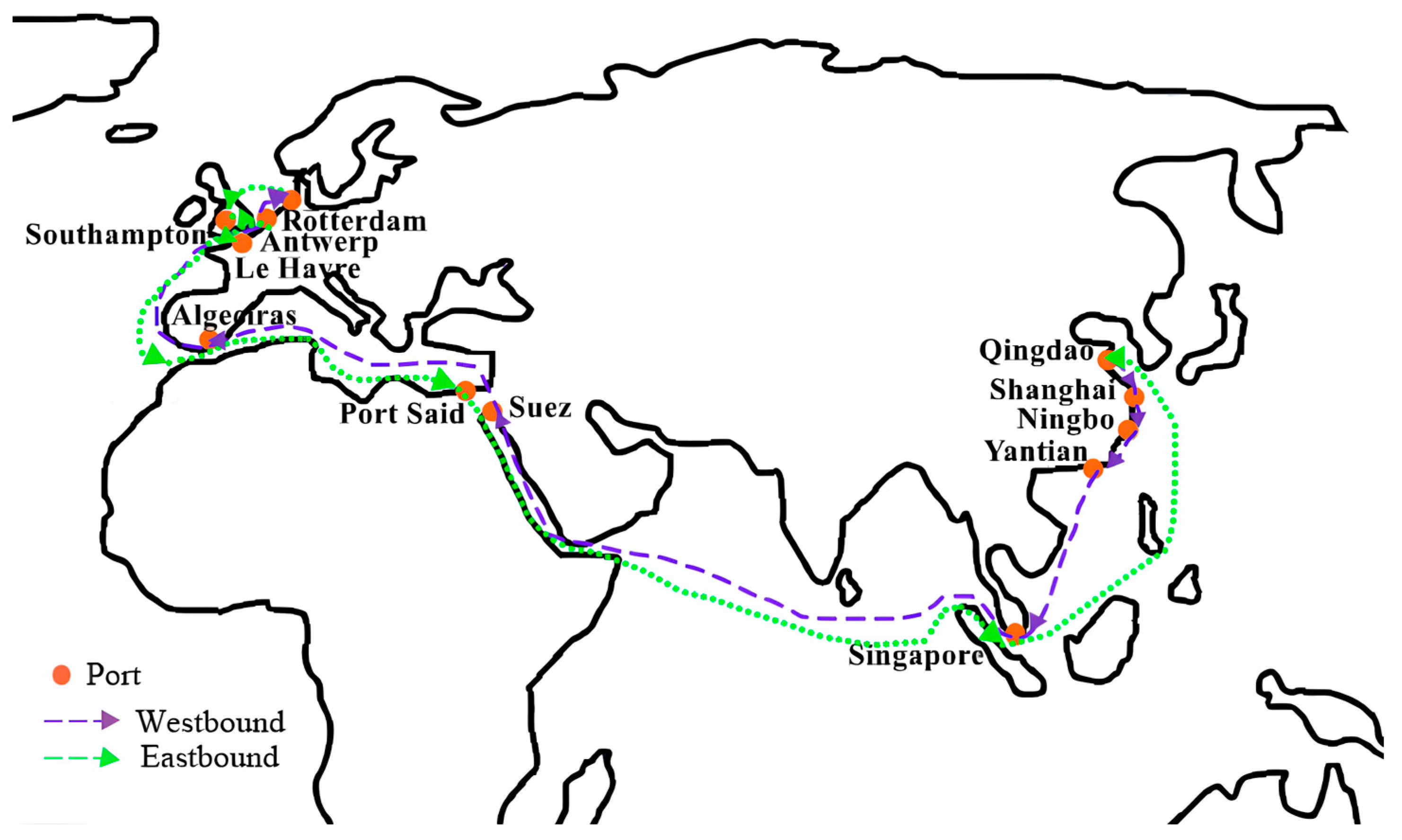
| 1 | Qingdao | 138 | 308 | 34 | 0 | 0 | 852 | 653 |
| 2 | Shanghai | 160 | 0 | 37 | 98 | 100 | 855 | 637 |
| 3 | Ningbo | 454 | 247 | 37 | 142 | 148 | 817 | 623 |
| 4 | Yantian | 44 | 1426 | 18 | 252 | 257 | 947 | 645 |
| 5 | Singapore | 0 | 5022 | 20 | 362 | 368 | 797 | 646 |
| 6 | Suez | 1939 | 88 | 12 | 652 | 660 | 1090 | 737 |
| 7 | Algeciras | 407 | 996 | 25 | 786 | 800 | 870 | 635 |
| 8 | Rotterdam | 251 | 0 | 119 | 952 | 961 | 819 | 581 |
| 9 | Southampton | 296 | 0 | 80 | 1095 | 1099 | 792 | 605 |
| 10 | Antwerp | 297 | 0 | 34 | 1210 | 1217 | 787 | 612 |
| 11 | Le Havre | 222 | 1031 | 43 | 1265 | 1279 | 810 | 618 |
| 12 | Algeciras | 1932 | 0 | 15 | 1371 | 1404 | 870 | 635 |
| 13 | Port Said | 0 | 5107 | 15 | 1516 | 1522 | 886 | 648 |
| 14 | Singapore | 33 | 2436 | 42 | 1888 | 1913 | 818 | 646 |
| 15 | Qingdao | -- | -- | 34 | 2120 | 2120 | 852 | 653 |
| No. | Port | Speed, Knots | Arrival Time, Hours | Whether or Not to Refuel | Bunkering Amount, Tons | |||
|---|---|---|---|---|---|---|---|---|
| ECA | MGO | MGO | ||||||
| 1 | Qingdao | 14.12 | 15.38 | 0 | 0 | 0 | 0 | 0 |
| 2 | Shanghai | 14.12 | -- | 63.79 | 0 | 0 | 0 | 0 |
| 3 | Ningbo | 14.12 | 15.38 | 112.12 | 0 | 1 | 0 | 1999.50 |
| 4 | Yantian | 14.12 | 15.38 | 197.32 | 0 | 0 | 0 | 0 |
| 5 | Singapore | -- | 15.38 | 311.12 | 1 | 0 | 2078.65 | 0 |
| 6 | Suez | 14.12 | 15.38 | 657.55 | 0 | 0 | 0 | 0 |
| 7 | Algeciras | 13.04 | 14.12 | 801.82 | 0 | 0 | 0 | 0 |
| 8 | Rotterdam | 13.04 | -- | 930.06 | 0 | 1 | 0 | 2637.72 |
| 9 | Southampton | 13.04 | -- | 1068.32 | 0 | 0 | 0 | 0 |
| 10 | Antwerp | 12.18 | -- | 1171.02 | 1 | 0 | 2700 | 0 |
| 11 | Le Havre | 13.04 | 14.12 | 1229.52 | 0 | 0 | 0 | 0 |
| 12 | Algeciras | 13.04 | -- | 1362.54 | 0 | 0 | 0 | 0 |
| 13 | Port Said | -- | 14.45 | 1526.62 | 0 | 0 | 0 | 0 |
| 14 | Singapore | 13.04 | 14.12 | 1903.19 | 0 | 1 | 0 | 600 |
| 15 | Qingdao | -- | -- | 2120 | -- | -- | -- | -- |
| Bunker Tank Capacity, Ton | Bunker Fuel Cost, USD | Bunker Tank Capacity, Ton | Bunker Fuel Cost, USD |
|---|---|---|---|
| 2000 | 7.25 × 10⁶ | 5000 | 6.94 × 10⁶ |
| 3000 | 6.95 × 10⁶ | 6000 | 6.96 × 10⁶ |
| 4000 | 6.94 × 10⁶ | 7000 | 6.97 × 10⁶ |
Disclaimer/Publisher’s Note: The statements, opinions and data contained in all publications are solely those of the individual author(s) and contributor(s) and not of MDPI and/or the editor(s). MDPI and/or the editor(s) disclaim responsibility for any injury to people or property resulting from any ideas, methods, instructions or products referred to in the content. |
© 2025 by the authors. Licensee MDPI, Basel, Switzerland. This article is an open access article distributed under the terms and conditions of the Creative Commons Attribution (CC BY) license (https://creativecommons.org/licenses/by/4.0/).
Share and Cite
Wang, Q.; Zhou, J.; Li, Z.; Liu, S. Towards Sustainable Shipping: Joint Optimization of Ship Speed and Bunkering Strategy Considering Ship Emissions. Atmosphere 2025, 16, 285. https://doi.org/10.3390/atmos16030285
Wang Q, Zhou J, Li Z, Liu S. Towards Sustainable Shipping: Joint Optimization of Ship Speed and Bunkering Strategy Considering Ship Emissions. Atmosphere. 2025; 16(3):285. https://doi.org/10.3390/atmos16030285
Chicago/Turabian StyleWang, Qin, Jiajie Zhou, Zheng Li, and Sinuo Liu. 2025. "Towards Sustainable Shipping: Joint Optimization of Ship Speed and Bunkering Strategy Considering Ship Emissions" Atmosphere 16, no. 3: 285. https://doi.org/10.3390/atmos16030285
APA StyleWang, Q., Zhou, J., Li, Z., & Liu, S. (2025). Towards Sustainable Shipping: Joint Optimization of Ship Speed and Bunkering Strategy Considering Ship Emissions. Atmosphere, 16(3), 285. https://doi.org/10.3390/atmos16030285