Time-Series Data-Driven PM_2.5 Forecasting: From Theoretical Framework to Empirical Analysis

Abstract

PM_2.5 in air pollution poses a significant threat to public health and the ecological environment. There is an urgent need to develop accurate PM_2.5 prediction models to support decision-making and reduce risks. This review comprehensively explores the progress of PM_2.5 concentration prediction, covering bibliometric trends, time series data characteristics, deep learning applications, and future development directions. This article obtained data on 2327 journal articles published from 2014 to 2024 from the WOS database. Bibliometric analysis shows that research output is growing rapidly, with China and the United States playing a leading role, and recent research is increasingly focusing on data-driven methods such as deep learning. Key data sources include ground monitoring, meteorological observations, remote sensing, and socioeconomic activity data. Deep learning models (including CNN, RNN, LSTM, and Transformer) perform well in capturing complex temporal dependencies. With its self-attention mechanism and parallel processing capabilities, Transformer is particularly outstanding in addressing the challenges of long sequence modeling. Despite these advances, challenges such as data integration, model interpretability, and computational cost remain. Emerging technologies such as meta-learning, graph neural networks, and multi-scale modeling offer promising solutions while integrating prediction models into real-world applications such as smart city systems can enhance practical impact. This review provides an informative guide for researchers and novices, providing an understanding of cutting-edge methods, practical applications, and systematic learning paths. It aims to promote the development of robust and efficient prediction models to contribute to global air pollution management and public health protection efforts.

1. Introduction

Globally, air pollution is one of the most pressing environmental challenges, profoundly impacting public health, ecosystems, and economic development [1,2,3,4,5]. In recent years, major pollutants such as particulate matter (PM_2.5), carbon dioxide (CO₂), and nitrogen dioxide (NO₂) have been closely associated with a variety of health problems at the urban and regional scales [6,7,8,9,10]. To mitigate these impacts and help policymakers make evidence-based decisions and management, accurate pollutant concentration predictions with high temporal and spatial resolution have attracted significant attention [11,12,13,14]. Spatial models such as land use regression (LUR) are often used to estimate PM_2.5 distribution with high spatial resolution. Reliable prediction models for short-term and long-term air quality forecasts can help response strategies, provide timely warnings to the public, and reduce exposure risks [15,16,17,18].

In air pollution forecasting research, time series data play a pivotal role. The concentrations of pollutants like PM_2.5, NO₂, and CO₂ exhibit temporal variations. They are closely associated with meteorological conditions (e.g., humidity, temperature, wind speed, and pressure) as well as human activities (e.g., traffic flow and industrial emissions) [19,20,21,22]. Early studies predominantly employed statistical and traditional machine learning methods, including linear regression [23,24,25], support vector machines (SVM) [26,27,28], naïve Bayes [29,30,31], random forests (RF) [32,33,34], and gradient-boosted trees (GBDT) [35,36,37]. These methods often relied on manually engineered features and achieved some success in short-term predictions of pollutant concentrations. Jeong et al., 2021 [38], applied simple linear regression (SLR) to forecast winter PM_2.5 concentrations in East Asia by correlating PM_2.5 levels with climate indices like ENSO and the Siberian high. Despite using a single predictor, the SLR model demonstrated a robust correlation (r > 0.72) with the observed PM_2.5 values and successfully captured abnormal winter PM_2.5 variability.

Gong et al., 2024 [39], used an enhanced SVM optimized by the Sparrow Search Algorithm (SSA) for PM_2.5 prediction. By integrating principal component analysis (PCA) into migrate data redundancy, the SSA-SVM showed excellent prediction accuracy, reduced computational complexity, and could effectively handle high-dimensional and nonlinear data. Tella et al., 2021 [40] used naïve Bayes, random forest, and K-nearest neighbor algorithms to predict PM₁₀ hotspots in Malaysia. Naïve Bayes achieved an overall accuracy of 91% but lagged behind other models regarding specificity and recall. Nevertheless, the study highlighted its utility for spatial assessments of air quality in urban areas. In a study by Chen et al., 2021 [41], random forests were combined with satellite-derived aerosol optical depth (AOD) data, meteorological parameters, and land use factors to estimate monthly PM_2.5 concentrations in Taiwan at a spatial resolution of 3 km. The model achieved an R² value of 0.82 and a root mean square error (RMSE) of 3.85 μg/m³ in cross-validation, outperforming pure machine learning methods. This hybrid approach improves prediction accuracy and considers complex terrain and topography. He et al., 2022 [42], used a boosted gradient-boosted decision tree (GBDT) model that used satellite-based AOD data and meteorological information to reconstruct high-resolution (1 km) PM_2.5 concentration data for China from 2015 to 2020. The model achieved an overall R² value of 0.92 and effectively simulated the spatial and temporal distribution of PM_2.5, providing insights into regional pollution trends.

However, as data become increasingly complex and heterogeneous, traditional models face limitations in capturing highly nonlinear patterns, long-term dependencies, and the coupled characteristics of multiple pollutants [43]. Over the past decade, deep learning techniques have emerged as a prominent focus in time series forecasting to overcome these limitations [44,45]. Convolutional neural networks (CNNs) leverage multilayer convolutional kernels to extract and learn local patterns. These networks effectively identify short-term trends in pollutant concentrations and offer new perspectives for capturing spatially localized features [46,47,48]. Recurrent neural networks (RNNs) [49,50,51] and their advanced extensions, namely long short-term memory (LSTM) [52,53,54] and gated recurrent units (GRUs) [55,56,57], excel in modeling the long-term dependencies within time series data and exhibit strong capabilities in addressing nonlinear air pollution forecasting problems. More recently, transformer models and attention mechanism-based approaches have transcended the sequential limitations of traditional RNN by enabling the parallel processing of long sequences and extracting remote dependencies through self-attention mechanisms [58,59,60].

In this context, hybrid and improved models are emerging, such as integrating traditional models like ARIMA and SVR with deep learning frameworks and ensemble learning approaches combining multiple deep learning models to enhance prediction accuracy and robustness [61,62,63,64]. However, deep learning and hybrid models still face challenges, including data scarcity, feature selection complexity, model interpretability, and high computational demands. In actual application scenarios, the absence of high-quality data and well-structured modeling processes can lead to deep learning models being susceptible to overfitting or being unable to accurately grasp the temporal variations in pollutant levels.

To systematically review the progress of this research field and explore future directions, we conducted a comprehensive review of the research on pollutant concentration prediction using time series analysis techniques. Using the Web of Science (WoS) database, 2327 journal articles published between 2014 and 2024 were retrieved and analyzed using the keywords “PM_2.5” and “time series”. We examined the selected literature in terms of methods, model development, data processing, and performance evaluation. This review is structured around four key dimensions:

1. Bibliometric Analysis: Using the CiteSpace (V6.4 R1) bibliometric tool, a comprehensive survey was carried out of research trends and trajectories in “air pollution prediction based on time series analysis”. This included time trends in publications, regional distribution, collaboration networks, keyword co-occurrence analysis, mutation word analysis, and time series cluster mapping.

2. Data Characteristics and Acquisition: By combing through existing studies, we summarize the types of data commonly used in PM_2.5 prediction, including ground monitoring data, meteorological information, remote sensing observations, and human activity-related data. Combined with the results of the quantitative literature research, we introduce various data types and their primary sources. The structure and characteristics of time series data and standard data processing methods are outlined.

3. Technical Overview: We outline the structure of deep learning models used in PM_2.5 time series forecasting (e.g., CNN, RNN, LSTM, and transformers) and their role in processing complex temporal features. Compared to large AI models with billions of parameters, the deep learning models used for PM_2.5 time series forecasting are usually smaller in scale. In the existing research, most models can be trained on CUDA-enabled GPUs, which has obvious advantages in terms of hardware cost and reproducibility. We study the advantages and disadvantages of various models in terms of feature extraction, prediction accuracy, computational efficiency, and their specific applications in air pollution forecasting.

4. Challenges and Future Prospects: We discuss unresolved challenges such as multi-source data integration, model interpretability and generalization, computational resource requirements, and algorithmic complexity. In addition, we discuss the potential of emerging technologies, such as meta-learning, reinforcement learning, graph neural networks, and multi-scale modeling, in advancing air pollution forecasting.

Based on a systematic synthesis and evaluation of the existing literature, this review provides a clear development trajectory of deep learning for air pollution prediction in recent years, as well as practical application cases. It provides a valuable reference for improving prediction accuracy, model robustness, and practical applicability. We hope this work will inspire researchers and practitioners to choose models, obtain and preprocess data, and explore new technologies.

2. Bibliometric Analysis

This survey systematically examines the research prospects and development trajectory of time series-based air pollution forecasting using bibliometric analysis and data visualization methods. CiteSpace [65], a well-known data visualization and analysis tool, was used to create a thematic knowledge graph highlighting the leading publications, the regional distribution of the research, and emerging frontiers in air pollution forecasting.

A comprehensive assessment of the relevant literature was conducted to help researchers track the latest progress and potential future trajectory of time series-based air pollution forecasting technology. The Web of Science Core Collection was searched using the terms “PM_2.5” and “Time Series” from 2014 to 2024. The selection of the 2014–2024 timeframe was based on two key considerations. First, for a systematic review, a ten-year timeframe can strike an appropriate balance between comprehensiveness and timeliness, ensuring that the study can capture the latest advances in PM_2.5 prediction. Second, deep learning-based methods first appeared in air quality prediction research around 2014 and have experienced rapid development since then. Prior to this, research mainly relied on traditional statistical and machine learning models. By selecting this timeframe, a better distinction can be made between traditional and emerging technologies. After eliminating duplicates, a total of 2327 journal articles were identified. Journal articles were selected as the primary data source for this study because they have a rigorous peer-review process that ensures scientific validity and methodological rigor. However, we also recognize the potential limitations of this approach and encourage readers to consider recent conference proceedings and preprint papers available on preprint platforms or from recent academic conferences. These sources often introduce cutting-edge research advances before they are officially published, providing valuable insights into the latest advances in the field.

The collected literature was comprehensively analyzed using CiteSpace (version 6.4. R1), focusing on five key dimensions: (1) chronological trends in publications, (2) geographic distribution and collaboration networks, (3) keyword co-occurrence networks, (4) mutation detection analysis, and (5) time series clustering plots. Publication trends indicate the intensity of academic involvement in the field. At the same time, the geographic analysis shows that air pollution forecasting is a global concern, with different levels of research investment in various countries. An analysis of keyword co-occurrence reveals core technical themes and temporal clustering plots graphically represent emerging research trajectories and frontiers.

This bibliometric approach is comprehensive and multifaceted, successfully illustrating the overall “landscape” of technical research on forecasting PM_2.5 and other air pollutants by utilizing time series datasets. The results help summarize the current achievements and shortcomings, identify potential directions for technological advancement, and provide valuable references for future research in this field.

2.1. Literature Trends

Figure 1 visually depicts the yearly publication yield and its variations in the realm of PM_2.5 time series prediction from 2014 to 2024. The data presented in the figure show an upward trend in the 2014–2021 period and a slow decline in 2021–2024.

In particular, between the years 2014 and 2015, there was a rise in the number of annual publications from 67 to 86. From 2016 onward, publication activity showed notable fluctuations while maintaining an overall upward momentum. After reaching 114 papers in 2016, it increased to 143 in 2018. The year of 2019 witnessed a substantial surge to 238 papers, nearly a 66% increase over 2018, suggesting heightened scholarly attention.

In 2020, publications continued their upward trend, reaching 240 papers. This is likely due to the impact of the global public health event of COVID-19, which further boosted research on air pollutants. In 2021, there was a more pronounced increase, with the number jumping to 363, indicating a significant increase in research output. Although there were slight declines in 2022 and 2023 to 347 and 344, respectively, these numbers are still much higher than in previous years, reflecting the extensive academic participation in the field.

While the counts for 2022 (347), 2023 (344), and 2024 (272) indicate a partial stabilization, they are still well above the levels of the mid-2010s, highlighting the ongoing and evolving nature of academic research in PM_2.5 time series forecasting.

2.2. Geographic Distribution of Research

Figure 2 shows the international cooperation network of countries involved in PM_2.5 time series prediction [65]. This analysis examines the distribution of publications by country based on the author affiliations recorded from the WOS dataset for the 2327 articles stated above. The Annual ring size represents the volume of publications from a particular country, and the link color (dark to light) represents the frequency of collaboration between countries (high to low). The color of the annual rings corresponds to the legend, and the color represents the publication date. From the information analysis in the figure, we can see that China (PEOPLES R CHINA, 1223) and the United States (USA, 534) occupy a central position, with relatively large node sizes, which indicates a more significant number of publications and greater influence in academic exchanges. Other countries, such as Australia (AUSTRALIA, 132), South Korea (SOUTH KOREA, 112), and England (ENGLAND, 109), also stand out, reflecting active research work and a clear trend of international cooperation in this field.

In addition, the purple rings around specific nodes indicate betweenness centrality [65]: this feature indicates that a country plays a vital “bridge” role in cross-national and cross-regional academic cooperation. For example, Germany, Australia, and France show relatively strong betweenness centrality, indicating their greater strength in connecting different research communities.

In general, the number and density of links between nodes indicate the frequency and closeness of scientific cooperation. The multiple connections between China and the United States point to frequent citation and joint publication activities, signaling robust scholarly interactions. Similarly, numerous European nations, such as Germany, France, Italy, and Sweden, are tightly interlinked, suggesting a certain degree of intra-regional synergy and knowledge exchange within the scope of research on PM_2.5 time series prediction.

The concentric color “year rings” on each node represents the year of publication. Darker tones correspond to earlier research results, while lighter tones represent newer research. These layered color gradients thus illustrate the changes in a country’s continuity over time and provide clues for tracking the evolution of academic focus.

In summary, the global pattern of the field shows a multi-center collaboration model with China and the United States at the core, as well as multiple interaction points across Europe, Australia, and other Asian countries. Countries with more obvious purple rings play a key role in cross-regional cooperation and knowledge dissemination, and the “year ring” color spectrum clearly shows the development of research activities and timelines in each country, ultimately providing a valuable reference for understanding the emerging trends in international academic partnerships and PM_2.5 time series forecasts.

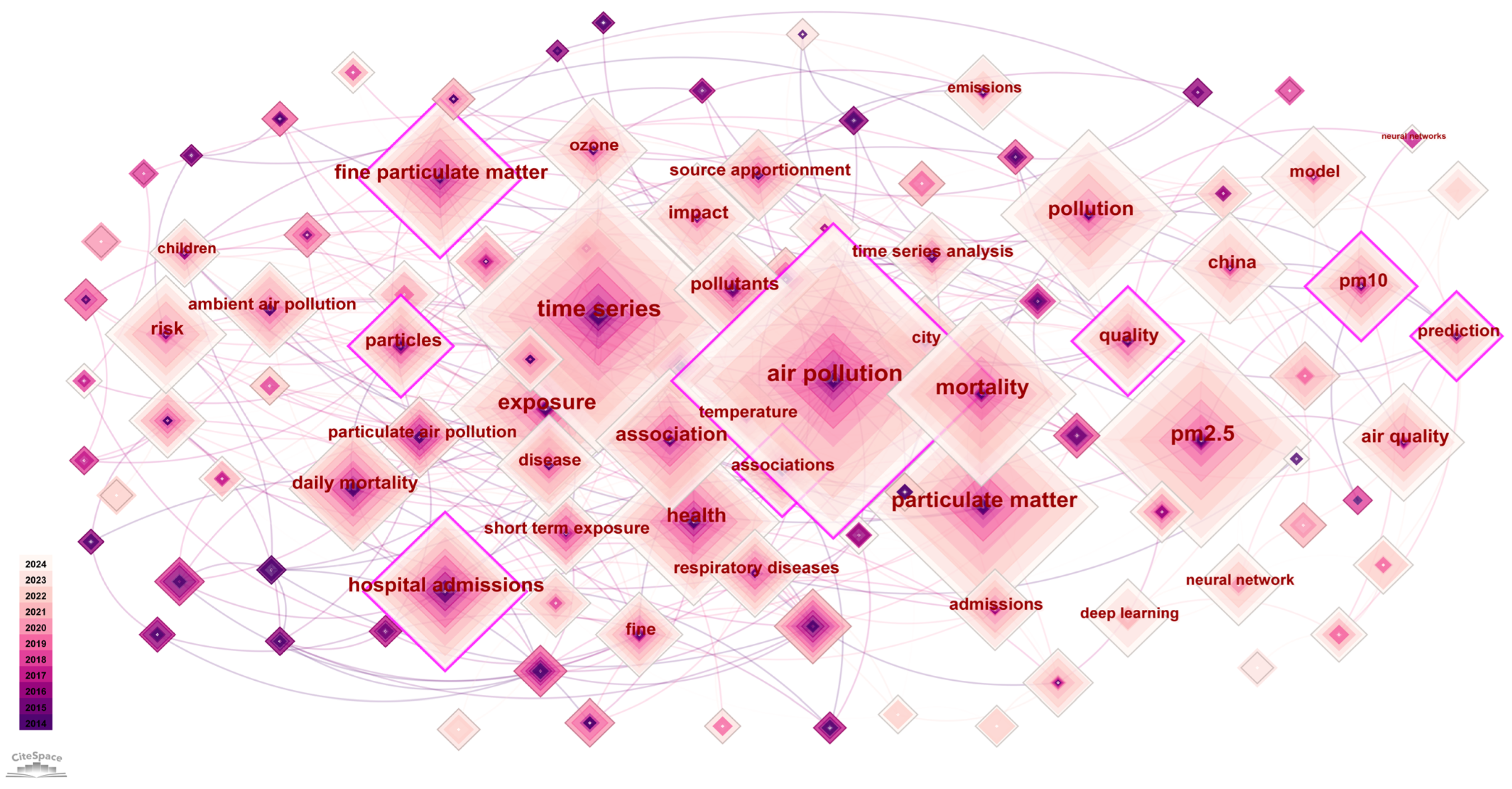
2.3. Keyword Co-Occurrence Analysis

In this survey, the data used were from 1 January 2014 to 30 December 2024 and keywords were extracted from 2327 articles as analysis data. Keyword co-occurrence analysis [65] using CiteSpace successfully highlighted the research priorities in PM_2.5 time series prediction. Figure 3 shows a keyword co-occurrence network centered on PM_2.5 time series prediction, providing insights into the core research topics and evolving methodological approaches in this field. In this image description, the size of each node is proportional to the number of articles containing the corresponding keyword. Some low-frequency words retain their spatial positions, but no specific words are displayed. The purple outer ring indicates keywords with a high betweenness centrality, meaning that they play a connecting role across multiple research topics. The interconnecting lines describe the relationship (appearing in the same article) between keywords, and the depth of the color (dark to light) represents the strength of the connection (high to low).

Health-related keywords (e.g., “mortality”, “number of hospitalizations”, “daily mortality”, and “respiratory diseases”) are all concentrated around the concept of disease impact. This co-occurrence pattern emphasizes the high importance the research community attaches to assessing public health risks and outcomes, indicating that quantifying the morbidity and mortality associated with PM_2.5 remains a key research goal.

In addition to the objective descriptive level of air pollution, the prominence of “model” (145 times) and “forecasting” (105 times) indicates that the main focus of the work is on the research and development of pollutant prediction models. Regarding the methodological level, “deep learning” (79 times) and “neural networks” (87 times) have become key computational tools, indicating that PM_2.5 research is increasingly data-oriented and combined with AI technology. The co-occurrence of these terms suggests that scholars are gradually applying and refining algorithmic models to improve prediction accuracy, adapt to complex nonlinear relationships, and handle large-scale datasets characteristic of air quality research.

Terms such as “exposure”, “risk”, “ambient air pollution”, and “daily mortality” frequently co-occur with major pollution and health descriptors. This phenomenon illustrates the close connection between environmental measurements (pollutant levels, composition, and distribution) and human health outcomes (hospital visits, mortality, and disease incidence). This convergence implies a holistic research framework in which scientists not only monitor PM_2.5 concentrations but also strive to correlate these levels with clinically meaningful endpoints.

CiteSpace’s color gradient, from darker tones for early publications to lighter tones for newer work, visualizes the evolution of the field. Traditional pollutant-related terms (e.g., “particulate matter”, “air pollution”) display darker color layers, emphasizing their longevity and dominance in the literature. In contrast, more recently emerging methods and topics like “deep learning” and “neural networks” often have lighter color layers, highlighting their relatively new but rapidly growing use in addressing PM_2.5-related challenges.

Overall, this co-occurrence network illustrates the dual focus of air pollution research focusing on the health-oriented dimensions (assessing exposure, risk, mortality, and disease outcomes) and the increasingly sophisticated computational methods used for AI modeling and forecasting pollution. These findings suggest that PM_2.5 scholarship has evolved from basic studies of pollutant impacts to data-intensive, algorithm-driven analyses designed to inform scientific understanding and policy decisions for better air quality management.

2.4. Mutant Terms

To present the evolution of keywords in this field, in this survey we used a list of mutation terms generated by CiteSpace, and the selected data were keyword data from 2327 articles retrieved from 2014 to 2024. CiteSpace’s mutation detection [65] is based on the discrete-time mutation detection model proposed by Kleinberg, which identifies significant frequency fluctuations in time series through state machines or hidden Markov models, used to identify keywords with a spike in usage over a period of time.

Table 1. Top 20 mutant keywords in PM_2.5 time series forecasting research.

Keywords	Year	Strength	Begin	End	2014–2024 *
fine particles	2014	13.6	2014	2018	▃▃▃▃▃▃▃▃▃▃▃▃
coarse particles	2014	12.74	2014	2019	▃▃▃▃▃▃▃▃▃▃▃▃
matter	2014	11.9	2014	2018	▃▃▃▃▃▃▃▃▃▃▃▃
case-crossover analysis	2014	9.41	2014	2017	▃▃▃▃▃▃▃▃▃▃▃▃
chemical composition	2014	9	2014	2018	▃▃▃▃▃▃▃▃▃▃▃▃
particulate air pollution	2014	8.53	2014	2018	▃▃▃▃▃▃▃▃▃▃▃▃
long-term exposure	2014	7.35	2014	2018	▃▃▃▃▃▃▃▃▃▃▃▃
United States	2015	11.46	2015	2019	▃▃▃▃▃▃▃▃▃▃▃▃
hospital admissions	2014	11.36	2015	2017	▃▃▃▃▃▃▃▃▃▃▃▃
chemical constituents	2015	6.95	2015	2017	▃▃▃▃▃▃▃▃▃▃▃▃
short term exposure	2014	10.87	2017	2020	▃▃▃▃▃▃▃▃▃▃▃▃
inflammation	2014	8.99	2017	2019	▃▃▃▃▃▃▃▃▃▃▃▃
cardiovascular mortality	2015	10.68	2018	2020	▃▃▃▃▃▃▃▃▃▃▃▃
burden	2019	7.24	2019	2021	▃▃▃▃▃▃▃▃▃▃▃▃
algorithm	2020	10.46	2020	2021	▃▃▃▃▃▃▃▃▃▃▃▃
models	2019	7.42	2021	2022	▃▃▃▃▃▃▃▃▃▃▃▃
machine learning	2022	11.85	2022	2024	▃▃▃▃▃▃▃▃▃▃▃▃
air pollutants	2016	11.8	2022	2024	▃▃▃▃▃▃▃▃▃▃▃▃
prevalence	2022	9.37	2022	2024	▃▃▃▃▃▃▃▃▃▃▃▃
neural network	2020	8.5	2022	2024	▃▃▃▃▃▃▃▃▃▃▃▃

* The purple bar indicates the peak mutation period. The two light-colored lines are both representing that the node was not in a “mutation” state at that time.

shows the top 20 keywords that show citation mutations in the PM _2.5 time-series prediction field, including their mutation intensity and time span (Begin-End). The timeline bar for each keyword indicates the time of its citation mutation, and the purple bar indicates the peak mutation period. The two light-colored lines are visualizations made by CiteSpace to distinguish adjacent time slices, both representing that the node was not in a “mutation” state at that time. These data provide insights into the emergence and evolution of key research topics in different periods. From a professional perspective, the following main trends can be drawn:

Between 2014 and 2018, keywords such as “fine particles” (strength = 13.6, 2014–2018), “coarse particles” (strength = 12.74, 2014–2019), and “particulate air pollution” (strength = 8.53, 2014–2018) indicate that the focus during this period was on studying particulate matter itself and the environmental or health effects it caused. It should be noted that in the search terms, “fine particles” and the topic “PM_2.5” are synonyms, so they are highly related. At the same time, health-related terms such as “long-term exposure” (strength = 7.35, 2014–2018), “short-term exposure” (strength = 10.87, 2017–2020), and “hospital admissions” (strength = 11.36, 2015–2017) highlight the development of interest from an epidemiological and public health perspective, focusing on the morbidity and hospitalization rates associated with PM_2.5 exposure.

The terms “chemical composition” (intensity = 9, 2014–2018), “chemical constituents” (intensity = 6.95, 2015–2017), etc., reflect the increasing interest in the study of PM_2.5 and its chemical composition. The keywords “inflammation” (intensity = 8.99, 2017–2019), “cardiovascular mortality” (intensity = 10.68, 2015–2020) further highlight the interest in the study of particulate matter and specific diseases.

The rapid growth of the keyword “United States” (Strength = 11.46, 2015–2019) indicates strong research activity in the region, which may be driven by extensive monitoring networks and open access data. The subsequent increase in “burden” (Strength = 7.24, 2019–2021) shows that research increasingly focuses on quantifying the disease burden generated by PM_2.5 pollution, reflecting the increasing impact of air pollution on socioeconomic costs and public health.

Keywords such as “models” (Strength = 7.42, 2019–2022) and “algorithm” (Strength = 10.46, 2020–2021) show significant citation bursts starting in 2019. This phenomenon reflects the academic community’s drive to develop and improve computational methods as the amount of air quality data increases and the overall research moves toward more systematic model-building.

Among the analysis results, “machine learning” (strength = 11.85, 2022–2024) and “neural network” (strength = 8.5, 2020–2024) show a high level of citation burst intensity in a relatively recent time frame. These terms mark the rapid rise in data-driven techniques and artificial intelligence technologies for modeling complex and nonlinear behaviors in PM_2.5 data, resulting in more accurate prediction models and enhanced analytical capabilities.

In summary, Table 1 illustrates a clear trajectory from the initial explorations of PM_2.5 composition and its health effects to epidemiological and public health assessments to a more recent focus on computational innovation. These keyword mutations indicate a development pattern from early studies of particulate matter properties and related health effects to the current dominance of big data resources and advanced artificial intelligence models. Over time, the direction of academic research on PM_2.5 has shifted from basic descriptive assessments to a more comprehensive approach that combines epidemiology, public health research, and cutting-edge deep learning. These developments have not only deepened our understanding of PM_2.5 dynamics and its health effects but also paved the way for more accurate modeling and robust policy interventions. With the expansion of monitoring coverage and the improvement in algorithmic complexity and computational efficiency, future research is likely to continue to refine our understanding of particulate matter pollution and its risks, thereby promoting further interdisciplinary collaboration and practical applications.

2.5. Clustering Timeline Mapping

To intuitively show the changing trends and relationships of keywords in research fields over time, this survey used Latent Semantic Indexing (LSI) [65] clustering in CiteSpace to group keywords into topic clusters based on their co-occurrence patterns. The dataset was divided into one-year intervals to show how keywords change over time. The input data were also the keyword data from the 2327 retrieved articles. As shown in Figure 4, this visualization provides a dynamic perspective on how the main concepts and research fields evolve over time. The clusters are numbered and arranged on the right side of the figure (#0–#9) according to their size. The horizontal axis corresponding to the cluster shows the keywords in the cluster, and the order of arrangement on the horizontal axis shows the time distribution characteristics of the keywords in the cluster. The keyword frequency is proportional to the size of the diamond icon. The purple outer circle also represents the betweenness centrality. Several noteworthy points can be observed by examining the clustering and time distribution of keywords.

The largest cluster (#0 “air pollution”) highlights the fundamental nature of air pollution research, with early research (around 2014–2016) focusing on broad descriptors such as “particulate matter” and “risk”. As the field progressed, researchers began to integrate health outcomes (e.g., “hospital admissions”, “risk factors”) and environmental indicators (e.g., “air quality”, “source apportionment”), revealing a research direction that links PM_2.5 pollution to relatable impacts on public health and ecological conditions.

The emergence of a cluster (#1 “deep learning”) highlights the growing popularity of data-driven techniques and advanced computational methods influenced by artificial intelligence technologies. Terms such as “machine learning”, “neural network”, and “algorithm” appear with high frequency starting around 2020. This development suggests that the primary research methodological trend is toward complex models that can capture nonlinearity, spatiotemporal variability, and large datasets compared to traditional statistical methods.

Clusters focused on specific diseases also stand out, with clusters (#2 “cardiovascular disease” and #8 “stroke”) reflecting interest in specific health effects of PM_2.5. Since 2015, terms such as “case crossover analysis”, “obstructive pulmonary disease” and “heart rate variability” have supported this research direction, indicating strong interdisciplinary collaborations between environmental science and medical research. The above three terms are closely linked in cluster #2. Over time, the emphasis on these health conditions has expanded from single conditions to systemic effects (e.g., “inflammation”, “respiratory diseases”, “mental disorders”). This phenomenon suggests that researchers emphasize that PM_2.5 exposure may lead to widespread adverse consequences.

Source research on air pollutants is also a focus, with clusters (#3 “source apportionment”, #7 “spatial variability”) showing research hotspots aiming to identify the spatial distribution characteristics of pollutant sources. Keywords such as “biomass burning”, “urban area”, and “chemical constituents” show specific research directions to quantify their spatial distribution. Investigations into spatial variability indicate that high-resolution monitoring and modeling are still needed in specific research implementations to allow for policymakers to target specific sources of PM_2.5 more effectively.

Clusters (#4 “particulate air pollution”, #6 “time series analysis”) demonstrate the critical role of time series techniques in understanding pollutant fluctuations and predicting near-term trends. Keywords such as “regression”, “models”, “time-series study”, and “atmospheric modeling” indicate ongoing methodological improvements from the technical side, including short- and long-term forecasting models that inform public health guidelines and regulatory strategies.

In recent years (2020–2024), the emergence of keywords such as “mental disorders” and “prevalence” indicates that researchers are increasingly studying the broader social and clinical impacts of PM_2.5 exposure while showing a cross-disciplinary research trend from environmental science to medicine.

In summary, the bibliometric analysis highlights the current status of PM_2.5 prediction research dominated by deep learning methods. The results of the timeline cluster analysis shown in Figure 4 show that, after 2020, terms such as “deep learning”, “neural network”, and “machine learning” have become the dominant themes in PM_2.5 prediction research, reflecting the shift to more complex and automated prediction models. Although the change in keywords from deep learning models such as CNN, RNN, and LSTM to Transformer is not directly reflected in the figure, its evolution trajectory can be observed from the evolution of the mainstream research literature in recent years.

It has been shown in the research that CNN can extract local temporal patterns in PM_2.5 data. CNN can extract features from time series data through one-dimensional CNN, or it can combine spatial information for multi-point prediction through two-dimensional CNN. Although CNN performs well in short-term prediction, its structural characteristics lack the ability to model time series. With the increase in data volume and the improvement in computing power, researchers have begun to adopt methods based on RNN and its variants (such as LSTM and GRU) to improve the modeling ability of long-term data. However, the RNN structure has the problem of gradient vanishing, which limits the effectiveness of the model in long time series predictions. To solve this problem, the temporal convolutional network (TCN) has gradually become a research hotspot for PM_2.5 prediction in recent years. TCN replaces the recurrent structure with causal convolution and dilated convolution, allowing the model to perform parallel calculations within a longer historical window while avoiding the gradient vanishing problem. TCN has achieved a better performance than LSTM in some time series tasks and has gradually been applied to air quality prediction tasks. In recent years, with the improvement in computing power and the rise in the Transformer architecture, researchers have begun to pay attention to the application of the self-attention mechanism to PM_2.5 prediction. Transformer has shown advantages in multiple time series prediction tasks due to its parallel computing ability and good long-distance dependency capturing ability. Although the current research is still dominated by LSTM, hybrid models combined with attention mechanisms (such as CNN-LSTM, and LSTM–Transformer) have become a new research trend. In general, PM_2.5 prediction methods are becoming more complex and more able to combine multi-source data.

3. Fundamentals of PM_2.5 Forecasting and Data Characteristics

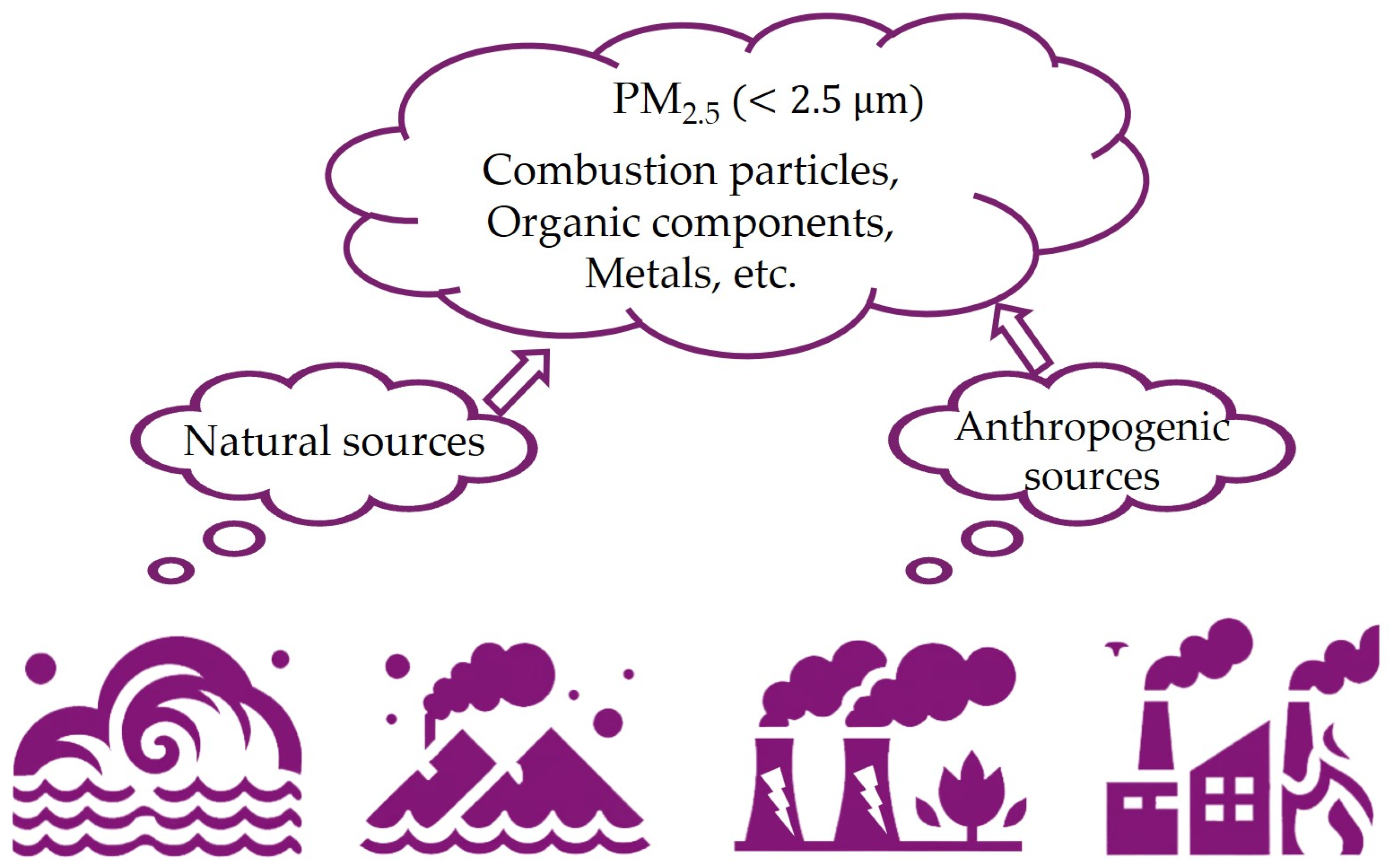
3.1. Physical and Chemical Properties and Formation Mechanism of PM_2.5

In environmental science, PM_2.5 is defined as particulate matter (solid or liquid droplets) with an aerodynamic diameter of less than or equal to 2.5 microns, an essential component of atmospheric aerosols. These tiny particles are characterized by their small size and large specific surface area, facilitating the adsorption of various toxic and harmful substances. Generally, the sources of PM_2.5 are natural and anthropogenic. Natural sources mainly include sandstorms, wildfires, ocean waves, and volcanic eruptions, and natural sources often show obvious seasonal and geographical characteristics. Anthropogenic sources include coal-fired power generation, industrial emissions, automobile exhaust, biomass burning, etc. These sources also have strong regional characteristics. The frequency and intensity of anthropogenic emissions are closely related to the level of human activity and the economic structure. Due to the size of PM_2.5 particles, they can stay in the atmosphere for a long time and can be transmitted over long distances, thus posing a major threat to the environment and human health [66,67,68,69]. Figure 5 presents an overview of the primary sources and components of PM_2.5.

From a chemical composition perspective, PM_2.5 typically includes nitrates, sulfates, organic carbon, elemental carbon, ammonium salts, and various heavy metal elements. The relative proportions of these components can differ considerably across regions and seasons. In areas with concentrated industrial activities, sulfates and elemental carbon often represent a larger fraction, whereas in agricultural regions or areas with frequent biomass burning, the organic carbon and nitrate compounds derived from nitrogen oxides may be more prevalent. Furthermore, atmospheric conditions such as temperature, humidity, wind speed, and topographic elements like boundary layer height can affect the dispersion and transformation of PM_2.5. As a result, its temporal and spatial distributions exhibit significant dynamic variability [70,71,72,73].

In terms of its formation mechanism, PM_2.5 includes primary particles emitted directly into the atmosphere and secondary particles produced through atmospheric chemical reactions involving precursors such as NO_x, SO₂, and volatile organic compounds (VOC). Secondary particulate matter accounts for a large proportion of PM_2.5, especially in cities or industrial areas. Organic pollutants can also form secondary organic aerosols through oxidative polymerization under photochemical conditions, further complicating the composition and concentration of PM_2.5. Unfavorable meteorological conditions (such as stable atmospheric stratification and low wind speed) can aggravate the local accumulation of these secondary products, leading to prolonged pollution events [74,75,76]. At the regional scale, PM_2.5 can be transported between different locations through atmospheric circulation. This cross-regional transport often results in high concentrations of PM_2.5 in some cities when external pollutants flow in, increasing the complexity of pollution control. Overall, the formation and evolution of PM_2.5 involve multiple interacting factors, including emissions from diverse sources, meteorological conditions, and atmospheric chemical reactions. For predictive modeling, accurately capturing these intricate spatiotemporal dynamics and physicochemical processes is of paramount importance.

3.2. Data Types and Sources

To build a reliable PM_2.5 prediction model, sufficient and high-quality data are an indispensable foundation. PM_2.5 data are often combined with multi-source and multi-scale information, including ground monitoring, meteorological, remote sensing, and anthropogenic activity data. This section will introduce various data types and their main sources in detail, combined with the results of the quantitative literature search. In Section 2.2, we conducted a bibliometric analysis to determine the distribution of research across countries. For consistency, we selected the top five countries with the highest number of publications as the primary source of the ground-based monitoring data used for our analysis. These publications mainly introduce the representative data acquisition channels in China, the United States, South Korea, Australia, Italy, and other countries with many publications on this subject.

3.2.1. Ground-Based Monitoring Data

Ground monitoring data are an important basis for air quality research, including particulate matter concentration and gaseous pollutant concentration. Particulate matter (including PM_2.5 and PM₁₀) data indicate the overall diffusion concentration of fine particles in the atmosphere. Gaseous pollutants, including nitrogen dioxide (NO₂), sulfur dioxide (SO₂), carbon monoxide (CO), and ozone (O₃), mainly come from industrial emissions, transportation, and combustion processes and have a significant impact on air quality and climate.

• China

Environmental quality data from across China are compiled and published at the China Environmental Monitoring Center, https://www.cnemc.cn/ (accessed on 26 February 2025). Users can access local environmental monitoring platforms in various provinces through this platform. This facilitates the retrieval of real-time and historical concentrations of air pollutants such as PM_2.5, making it suitable for large-scale, long-term studies [77,78,79].

• United States

Environmental Protection Agency (EPA) Air Quality System (AQS) provides air quality monitoring data from all U.S. states, including hourly or daily average concentrations of airborne contaminants such as PM_2.5, O₃, PM₁₀, and NO₂. Researchers can search for and download historical data from the EPA website, https://www.epa.gov/outdoor-air-quality-data (accessed on 8 January 2025) [80,81,82].

• Australia

Australia lacks a unified national platform for air quality monitoring data. Each state or territory’s environmental protection agency independently manages and provides access to monitoring data. Online air quality data retrieval services are available for various regions [83,84,85,86,87]. The primary sources are detailed in

Table 2. Australian state air quality data sources.

State	Data Source
Victoria	https://www.epa.vic.gov.au/for-community/airwatch (accessed on 8 January 2025)
New South Wales	https://www.airquality.nsw.gov.au/air-quality-in-my-area/concentration-data (accessed on 8 January 2025)
Queensland	https://apps.des.qld.gov.au/air-quality/ (accessed on 8 January 2025)
Western Australia	https://www.wa.gov.au/service/environment/environment-information-services/air-quality (accessed on 8 January 2025)
South Australia	https://www.epa.sa.gov.au/environmental_info/air_quality/new-air-quality-monitoring (accessed on 8 January 2025)

.

• Republic of Korea

Managed by the Ministry of Environment (MOE), the AirKorea website, https://www.airkorea.or.kr/web/ (accessed on 8 January 2025) provides nationwide air quality monitoring data, including PM_2.5, PM₁₀, SO₂, O₃, and NO₂. The dataset is updated frequently, allowing researchers to access daily averages or hourly measurements [88,89,90].

• Italy

The Sistema Nazionale per la Protezione dell’Ambiente (SNPA) network, established by national and regional environmental agencies in Italy, monitors and publishes real-time and past data on key pollutants like PM_2.5, NO₂, and O₃. The data can be accessed via the official website, https://www.snpambiente.it/prodotti/previsioni-qualita-dellaria-in-italia/ (accessed on 8 January 2025) or through portals shared with the European Union [91,92,93].

3.2.2. Meteorological Data

Meteorological factors include humidity, wind speed, temperature, air pressure, etc. These factors will significantly affect the spatiotemporal distribution and chemical changes in PM_2.5. Therefore, obtaining high-quality, multi-period, and appropriate spatial resolution meteorological data is essential for establishing an accurate PM_2.5 prediction model. The following section will introduce the main meteorological data collected from various countries and various reanalysis platforms.

• China

The National Meteorological Information Center, http://data.cma.cn/ (accessed on 8 January 2025) allows users to search for and download publicly available ground station observations, radar, and satellite data. Comprehensive meteorological observation data for China, including historical and real-time records of temperature, humidity, precipitation, wind direction, and wind speed, can be accessed through this platform [94,95,96].

• United States

The National Centers for Environmental Information, https://www.ncei.noaa.gov/ (accessed on 8 January 2025) provides ground observation, climate data, satellite, and radar for the United States and the globe. With a wide temporal range and diverse data types, researchers can retrieve and download data such as the temperature, wind, and precipitation for specific regions and time periods [97,98,99].

• Australia

The Bureau of Meteorology, http://www.bom.gov.au/ (accessed on 8 January 2025) offers real-time weather forecasts, observations, radar images, and a variety of historical meteorological data for Australia. Through the “Climate and Past Weather” section, users can download conventional meteorological elements like temperature, precipitation, wind direction, and speed by station and time [100,101].

• Republic of Korea

The Korea Meteorological Administration, https://www.kma.go.kr/ (accessed on 8 January 2025) provides nationwide weather forecasts, station observation data, and climate statistics. Historical and real-time observation data can be accessed through the “Data Service” or “Open Meteorological Data Portal”, https://data.kma.go.kr/cmmn/main.do (accessed on 8 January 2025) [102,103,104].

• Italy

The Italian Meteorological Service, http://www.meteoam.it/ (accessed on 8 January 2025) provides nationwide weather forecasts, monitoring, and warning information. Historical observation data are available for some regions. While the main pages are predominantly in Italian, specific observation data can be located using the site map or keyword search [105,106,107].

3.2.3. Reanalysis Data

Since some areas have no dedicated detection sites, processed reanalysis data are essential for large-scale or cross-regional studies, especially in areas with sparse ground observations. These datasets are generated by absorbing data from multiple sources, including ground observations, satellite data, and model simulations, ensuring comprehensive spatial and temporal coverage. Several commonly used Reanalysis datasets are introduced below, as follows:

• ERA5 (European Centre for Medium-Range Weather Forecasts, ECMWF)

Website: https://cds.climate.copernicus.eu/ (accessed on 8 January 2025)

ERA5 features a high spatial resolution (~0.25° × 0.25°) and hourly temporal resolution and provides a wide range of meteorological elements, including temperature, precipitation, humidity, wind direction, boundary layer height, and some aerosol data [108,109,110].

• MERRA-2 (NASA)

Website: https://gmao.gsfc.nasa.gov/reanalysis/MERRA-2/ (accessed on 8 January 2025)

MERRA-2 covers a global domain, with reanalysis starting in 1980 and continuing to the present. It includes atmospheric composition (gasses and aerosols) and standard meteorological elements, making it valuable for aerosol–meteorology coupling studies [111,112,113].

• JRA-55 (Japan Meteorological Agency)

Website: https://jra.kishou.go.jp/JRA-55/index_en.html (accessed on 8 January 2025)

Released by the Japan Meteorological Agency, this dataset has provided global meteorological information since 1958. It has relatively high simulation accuracy in East Asia, making it a complementary dataset to CMA observations [114,115,116].

• NCEP/NCAR Reanalysis and CFSR (NOAA)

Websites: https://psl.noaa.gov/data/gridded/data.ncep.reanalysis.html, (accessed on 8 January 2025)

https://rda.ucar.edu/datasets/ds093.0/ (accessed on 8 January 2025)

This dataset, developed by NOAA and NCAR, is suitable for long-term meteorological statistics and global comparative studies [117,118,119].

3.2.4. Remote Sensing Data

Ground-based monitoring data are usually difficult to apply when conducting research covering a large area because of their coverage and uneven distribution. Therefore, remote sensing data are more suitable for large-scale atmospheric observations. For PM_2.5 prediction and analysis, remote sensing data mainly focus on aerosol optical thickness and gaseous precursors (such as SO₂, NO₂, and O₃). These data can be integrated and adjusted with ground-based monitoring and meteorological data to achieve a balance between temporal and spatial coverage and fine precision. Below, commonly used remote sensors and data acquisition platforms are introduced.

• NASA and U.S.-Based Platforms

The National Aeronautics and Space Administration (NASA) operates some of the most representative satellites and sensors, including the Moderate Resolution Imaging Spectroradiometer (MODIS), onboard the Terra (morning overpass) and Aqua (afternoon overpass) polar-orbiting satellites [120]. MODIS provides global AOD data products, including MOD04 (Terra) and MYD04 (Aqua) [121,122].

Researchers can search and download these products via the LAADS DAAC (Level-1 and Atmosphere Archive & Distribution System Distributed Active Archive Center) website, https://ladsweb.modaps.eosdis.nasa.gov/ (accessed on 8 January 2025) or the NASA Earthdata platform, https://earthdata.nasa.gov/ (accessed on 8 January 2025). For large-scale data access, dedicated APIs are also available.

In addition to MODIS, NASA collaborates with the National Oceanic and Atmospheric Administration (NOAA) on the Suomi-NPP and NOAA-20 polar-orbiting satellite missions. The Visible Infrared Imaging Radiometer Suite (VIIRS) sensor aboard these satellites excels in aerosol observations, nighttime light detection, and fire point identification [123,124,125]. VIIRS Level 2/3 AOD products are also available through LAADS DAAC and Earthdata. Additionally, the Ozone Monitoring Instrument (OMI) onboard the Aura satellite specializes in atmospheric composition monitoring, including total ozone columns and gaseous precursors like NO₂ and SO₂ [126,127,128]. Access to these data is available via NASA’s GES DISC, https://disc.gsfc.nasa.gov/ (accessed on 8 January 2025), and initial visualization and statistical analyses can be performed using the Giovanni online analysis platform, https://giovanni.gsfc.nasa.gov/ (accessed on 8 January 2025).

• European Platforms and ESA

The European Space Agency (ESA) plays a key role in atmospheric monitoring and Earth observation, and the Copernicus program is a cornerstone program. The program is led by the European Union and supported by ESA’s technical and management expertise, including a series of Sentinel satellites.

Among them, the Sentinel-3 satellite is equipped with the Ocean and Land Color Instrument (OLCI) and the Sea and Land Surface Temperature Radiometer (SLSTR) to monitor the characteristics of aerosols and clouds [129,130]. The Sentinel-5P satellite is equipped with the Tropospheric Monitoring Instrument (TROPOMI), which can perform high-resolution observations of atmospheric gasses such as NO₂, SO₂, CO, and O₃. These data are of great value for studying the spatial dispersion and transport of PM_2.5-related precursors [131,132,133].

Sentinel products are accessible to researchers through the Copernicus Open Access Hub, https://scihub.copernicus.eu/ (accessed on 8 January 2025). For near-real-time and historical analyses of aerosol or PM_2.5 concentrations, the Copernicus Atmosphere Monitoring Service (CAMS), https://atmosphere.copernicus.eu/ (accessed on 8 January 2025) provides integrated products from satellite observations and numerical model assimilation [134]. These resources can also be accessed through the Atmospheric Data Store (ADS), facilitating comparison and integration with ground-based and other satellite data.

In addition, the European Space Agency’s Climate Change Initiative (CCI), https://climate.esa.int/ (accessed on 8 January 2025) provides high-quality, long-term standardized datasets for the study of climate trends and environmental change [135].

The European Organisation for the Exploitation of Meteorological Satellites (EUMETSAT), https://www.eumetsat.int/ (accessed on 8 January 2025) manages the Meteosat and Metop satellites. Researchers can access high-frequency atmospheric monitoring data on clouds, aerosols, and wind fields [136].

• NOAA and Other International Platforms

The National Oceanic and Atmospheric Administration (NOAA) operates extensive remote sensing programs and collaborates internationally. Its Comprehensive Large Array-data Stewardship System (CLASS), https://www.class.noaa.gov/ (accessed on 8 January 2025) is an integrated platform for retrieving data from polar-orbiting and geostationary satellites [137]. Researchers can access datasets from missions such as POES (Polar Orbiting Environmental Satellites), GOES (Geostationary Operational Environmental Satellites), Suomi-NPP, and NOAA-20, covering multidimensional observations of aerosols, clouds, precipitation, and sea surface temperature.

Through cooperation with NASA, NOAA’s VIIRS data can also be accessed and obtained through the CLASS platform. In addition, researchers can access datasets from instruments such as OMI and reanalysis products such as MERRA-2 through international projects such as NASA’s Goddard Earth Science Data and Information Service Center (GES DISC), https://disc.gsfc.nasa.gov/ (accessed on 8 January 2025). These data have made important contributions to promoting cross-regional and global studies of aerosol and PM_2.5 concentrations.

• Google Earth Engine

Google Earth Engine (GEE) is a cloud-based geospatial processing platform that provides access to a wide range of remote sensing datasets and provides powerful tools for large-scale geospatial analysis. Through GEE’s JavaScript and Python APIs, researchers can perform instant computation, time series analysis, and machine learning operations without having to store large amounts of data locally. The platform can quickly extract, preprocess, and fuse multi-source satellite observation data. In practice, researchers can explore and visualize these datasets on an interactive code editor, https://earthengine.google.com/ (accessed on 8 January 2025).

3.2.5. Socioeconomic and Anthropogenic Activity Data

Socioeconomic and human activity data related to the anthropogenic factors of PM_2.5 plays an indispensable role in predicting PM_2.5 concentrations. These data help researchers better understand the sources and distribution of pollutant emissions, especially in related studies such as industrial emissions and urbanization. Compared with meteorological or remote sensing data alone, socioeconomic data provide an additional dimension that can reveal deeper nonlinear relationships and potential causal mechanisms, thereby improving the accuracy and interpretability of prediction models.

• Traffic Data

Traffic data are among the most used components of socioeconomic datasets. Urban traffic departments or internet mapping platforms (e.g., Amap and Baidu Maps in China or traffic department websites in various U.S. states) often publish real-time or near-real-time information on vehicle flow, congestion indices, and vehicle speeds on major corridors. By correlating such traffic data with monitored PM_2.5 concentrations, researchers can preliminarily evaluate the relative contribution of vehicle emissions to local air pollution [138,139,140].

• Industrial Emissions and Energy Consumption

Industrial emissions and energy consumption data are another major source of socioeconomic and anthropogenic activity information, reflecting how energy structures, production scales, and technological levels impact PM_2.5 concentrations. Many countries’ emission inventories or pollution source registries record data on industrial emissions, emission types, and geographical locations.

Examples include China’s enterprise pollution permit platform [141], the U.S. Environmental Protection Agency (EPA) National Emissions Inventory (NEI) [142], Australia’s National Pollutant Inventory (NPI) [143], and industrial emissions registries in South Korea [144] and Italy [145]. These inventories often detail SO₂, NO_x, and VOC emissions, which are key contributors to the formation of secondary particulate matter.

In addition, annual or quarterly energy industry reports released by the government can also be used for model analysis. Such reports usually include statistics on coal, oil, and natural gas consumption and the composition of power generation. Correlating these macro-statistics with changes in PM_2.5 concentrations over the corresponding period can reflect the cyclical or trend-based relationship between economic activities and environmental quality.

• Population and Land Use/Land Cover Data

Socioeconomic activities directly lead to urban expansion, increased population density, and increased building density [146,147]. Such urbanization factors will have a negative impact on air quality. Usually, national statistical bureaus, geographic information departments, or academic databases store and provide census data, urban boundary data [148], and land use classification data [149] from different years. By overlaying these indicators with air pollution data, researchers can explore the spatial relationship between urbanization rate, population density, and PM_2.5 concentration. Furthermore, they can explore the differences in pollution distribution between industrial areas, transportation corridors, and residential areas.

Many cities’ official Geographic Information Systems (GIS) offer layered data on buildings, road networks, green spaces, and water bodies. Combined with high-resolution remote sensing images, this enables the detection of human activity patterns and potential pollution origins across various regions [150,151]. Furthermore, for European studies, the Corine Land Cover dataset from the Copernicus Land Monitoring Service provides harmonized land cover and land use data across multiple reference years, enabling cross-regional comparisons and integrated air pollution analyses [93]. This dataset is accessible via the Copernicus website, https://land.copernicus.eu/en/products/corine-land-cover (accessed on 8 January 2025), offering both historical and current land cover classifications.

3.3. Data Quality and Preprocessing

Ensuring data quality and applying proper preprocessing techniques are fundamental steps before modeling and analyzing PM_2.5 time-series data. During the data collection process, various factors—such as sensor malfunctions, communication interruptions, and extreme weather conditions—may introduce missing values, noise, and outliers into the raw data. Including such problematic data in models without appropriate handling can compromise the credibility of the prediction results.

This section explains key steps in data preprocessing, including missing data imputation, outlier and noise detection, denoising, stationarity transformation, feature selection, and normalization.

3.3.1. Missing Data Imputation

PM_2.5 concentration data often contain missing values, either sporadically or over continuous time periods, due to equipment maintenance or sensor failures. Leaving these missing periods unaddressed or simply deleting them may introduce biases during model training or prediction phases. Common imputation methods include simple interpolation techniques [152] and more sophisticated machine learning-based approaches [153,154]. In order to minimize errors, the imputed results should be cross-validated against adjacent time periods or data from nearby monitoring stations.

3.3.2. Outlier and Noise Detection

Sensor readings may be missing during operation due to external interference such as electromagnetic interference, equipment damage, etc. Sensor readings may have sudden peaks or distorted extreme values under abnormal weather conditions or equipment aging. In some datasets, missing value filling methods are also a research focus, and some abnormal extreme values are difficult to distinguish from actual pollution peaks. Such missing values and abnormal extreme values require a comprehensive evaluation, including meteorological conditions, observation data from neighboring stations, or historical statistical distributions. Common techniques for detecting outliers include box plots, 3σ rules, or clustering/distance-based algorithms such as DBSCAN [155,156].

3.3.3. Denoising and Stationarity Transformation

PM_2.5 data in long-term time series often exhibit non-stationary properties, where the mean and variance of the data distribution vary over time. Traditional statistical models (such as ARIMA) require the data to be roughly stationary [157]. Even when using advanced deep learning models, improving the stationarity of the data can reduce errors caused by seasonality or trends during training.

Techniques such as differencing, logarithmic transformation, or wavelet decomposition are commonly employed to mitigate trends and seasonal components. Techniques can be applied for high-frequency noise, including moving average filtering, wavelet thresholding, or exponential smoothing [158]. Specifically, differencing is effective when strong nonstationarity is present and helps stabilize the mean by removing long-term trends. Logarithmic transformations are useful for normalizing skewed distributions and dealing with heteroskedasticity. Wavelet decomposition allows for multi-resolution analysis, making it ideal for capturing both global and local patterns. For high-frequency noise reduction, moving average filtering can smooth short-term fluctuations while preserving the overall trend. Wavelet thresholding selectively removes noise without affecting key trends. Exponential smoothing is well-suited to short-term predictions as it gives greater weight to recent values. In practice, the data preprocessing method should be selected based on the specific characteristics of the dataset and the task objectives.

The denoising and stationarity steps may be simplified if the subsequent model can automatically extract multi-scale features (e.g., LSTM, Transformer). However, it is still advisable to evaluate the impact of noise levels and non-stationarity during the exploratory data analysis stage [159].

3.3.4. Feature Engineering and Normalization

In addition to PM_2.5 concentration, meteorological data (e.g., wind speed and direction, temperature) and socioeconomic activity data (e.g., traffic flow, emission inventories, population density) are often used as input features for models. During multi-source data integration, if a large number of redundant or weakly correlated candidate features exist, techniques such as Principal Component Analysis (PCA), Maximum Relevance Minimum Redundancy (mRMR), or machine learning algorithms based on feature importance (e.g., random forests, XGBoost) can be used for feature selection and dimensionality reduction, thereby reducing the risk of overfitting [160,161,162].

In different types of data series, feature values often vary greatly in magnitude and scale. For example, temperature is usually within a few tens of degrees, traffic volume ranges from thousands to tens of thousands, and some meteorological variables may exceed the kilometer level. To ensure the stability of model training and accelerate convergence, it is common practice to apply normalization or standardization to all features, such as minimum–maximum normalization or Z-score normalization.

This approach allows the model to fairly evaluate the contribution of each feature to the prediction and avoid being dominated or masked by features with too large values [163].

3.4. Common Evaluation Metrics in Prediction Tasks

Choosing accurate and appropriate evaluation metrics is critical when evaluating model quality and diagnosing the effectiveness of data preprocessing strategies. When using deep learning models to predict PM_2.5 time series data, common evaluation metrics include mean square error (MSE), root mean square error (RMSE), mean absolute error (MAE), and mean absolute percentage error (MAPE), each of which has its own focus and scope of application [164].

Comparing these metric values can quantify the performance of different models. In practice, it is possible to evaluate how missing data interpolation methods, outlier handling, or stabilization affect model performance, which can help to conduct a deeper analysis of the causes and select strategies.

• Mean Squared Error

As one of the foundational metrics for regression models, MSE quantifies the mean of the squared differences between forecasted and actual values. A lower MSE value indicates a reduced overall prediction bias. The definition of MSE is shown in Equation (1):

$$\mathrm{M}\mathrm{S}\mathrm{E}={\displaystyle \frac{1}{n}}\sum _{i=1}^n{({\widehat{y}}_i-y_i)}^2$$

(1)

where $n$ represents the total count of samples, and $y_i$ and ${\widehat{y}}_i$ represent the true value and predicted value, respectively. Since MSE is particularly susceptible to outliers, the presence of extreme errors can substantially increase the MSE.

2.

Root Mean Squared Error

The RMSE is derived by taking the square root of the MSE, providing a more direct sense of the prediction error in the same unit as the original data. It is defined as shown in Equation (2):

$$\mathrm{R}\mathrm{M}\mathrm{S}\mathrm{E}=\sqrt{{\displaystyle \frac{1}{n}}\sum _{i=1}^n{({\widehat{y}}_i-y_i)}^2}$$

(2)

Because RMSE shares the same units as the predicted target (for instance, $\mathsf{\mu }\mathrm{g}/{\mathrm{m}}^3$ for PM_2.5 concentration), it is more interpretable for practical applications. Like MSE, RMSE also responds strongly to large or extreme errors.

3.

Mean Absolute Error

Unlike MSE and RMSE, which use squared errors, MAE employs the absolute difference, making it somewhat less sensitive to outliers. It is formulated as Equation (3):

$$\mathrm{M}\mathrm{A}\mathrm{E}={\displaystyle \frac{1}{n}}\sum _{i=1}^n|{\widehat{y}}_i-y_i|$$

(3)

MAE offers a direct assessment of the average magnitude of prediction error in absolute terms. Researchers often use RMSE together with MAE to evaluate both overall error and extreme deviations.

4.

Mean Absolute Percentage Error

When focusing on relative errors—particularly when dealing with smaller concentration values—MAPE helps quantify the percentage deviation between predictions and true values. Its definition is shown in Equation (4):

$$\mathrm{M}\mathrm{A}\mathrm{P}\mathrm{E}={\displaystyle \frac{100\%}{n}}\sum _{i=1}^n\left|{\displaystyle \frac{{\widehat{y}}_i-y_i}{y_i}}\right|$$

(4)

MAPE provides a more intuitive “sense of proportion” for predictive errors. However, when $y_i$ is close to zero, MAPE may become unstable or lose meaning, calling for improved metrics (e.g., sMAPE) to handle such situations.

5.

Coefficient of Determination ($R^2$)

In some research, $R^2$ is used to assess the ratio of variance within the true values that are accounted for by the model. A figure nearing 1 signifies a superior fit. It is shown in Equation (5):

$$R^2=1-{\displaystyle \frac{{\sum }_{i=1}^n{({\widehat{y}}_i-y_i)}^2}{{\sum }_{i=1}^n{(y_i-\overline{y})}^2}}$$

(5)

where $\overline{y}$ is the mean of the true values. Note that for time-series forecasts, $R^2$ can occasionally become negative, indicating that the model might underperform for even a naive mean prediction. It should thus be interpreted alongside RMSE and MAE.

4. Deep Learning for PM_2.5 Time Series Forecasting

Commonly used air pollution data, including PM_2.5, often exhibit significant spatiotemporal heterogeneity and uncertainty. Traditional regression models or machine learning methods that rely on manually designed feature engineering have difficulty capturing highly nonlinear temporal dependencies for data-specific seasonal patterns or sudden events.

In contrast, deep learning models use a multi-layer network architecture to perform end-to-end feature extraction, enabling them to reveal the complex coupling relationships between multiple data types, such as PM_2.5, meteorological variables, and socioeconomic activity data. These deep learning models also perform well in training on large-scale, long-term datasets, achieving robust fitting and generalization capabilities [165,166,167,168,169].

Furthermore, deep learning models can effectively handle integrated multi-source datasets with large data volumes, which were previously difficult to process using traditional statistical methods. This development creates important opportunities for more accurate PM_2.5 predictions over a wider range of spatial and temporal scales.

On this basis, academic scholars in related fields have conducted in-depth research on the use of different deep learning structures for single-step and multi-step prediction tasks related to PM_2.5 prediction in recent years. These architectures include CNN and RNN and their enhanced variants, such as LSTM and GRU. There are also the latest methods, such as temporal convolutional network (TCN) and Transformer model based on the attention mechanism.

In this section, we will explore the principles and structural characteristics of each network architecture in depth and visualize the model architecture. In addition, we also show specific research cases and references to illustrate their real-world applications and performance results.

4.1. RNN and Its Improvements (LSTM, GRU)

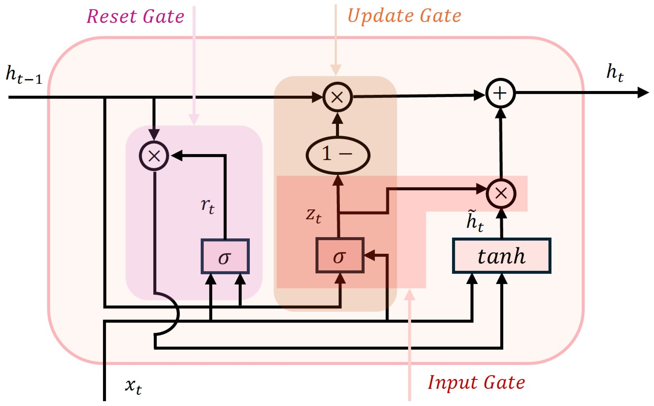
4.1.1. Model Structure and Principle Description (RNN, LSTM, and GRU)

RNN is a widely used deep learning architecture for modeling sequential data. Due to its sensitivity to sequence order and time, it was first widely used in natural language processing tasks. As research progressed, it was gradually found that its characteristics were also applicable to meteorological problems strongly related to time series. The core mechanism of RNN is to use the hidden state of the previous time step and the current input to capture the temporal dependency in the sequence. This mechanism adds a correlation between different inputs. Figure 6 shows the basic architectural layout of RNN.

The update of the hidden state is governed by Equation (6):

$$a^{⟨t⟩}=g_h\left(W_{aa}{a}^{⟨t-1⟩}+W_{ax}{x}^{⟨t⟩}+b_a\right)$$

(6)

where $a^{⟨t⟩}$ represents the hidden state at the current time $t$; $x^{⟨t⟩}$ represents the input at the current time $t$.

The computation at the output layer follows Equation (7):

$${\widehat{y}}^{⟨t⟩}=g_o\left(W_{ya}{a}^{⟨t⟩}+b_y\right)$$

(7)

where ${\widehat{y}}^{⟨t⟩}$ denotes the prediction of the output at the present moment. In practice, RNN stores time series information through the hidden state of the recurrent connection, which can capture the short-term changes in PM_2.5 concentration. $x^{⟨t⟩}$ is the input of the current time step (such as PM_2.5 concentration, temperature, etc.); $a^{⟨t⟩}$ is the hidden state of the current time step; ${\widehat{y}}^{⟨t⟩}$ is the predicted PM_2.5 value.

The parameters involved are defined as indicated in

Table 3. Common parameters of RNNs.

Parameter	Definition	Description
$W_{aa}$	Weight matrix from the previous hidden state to the current hidden state	Maps the previous hidden state $a^{⟨t-1⟩}$ to the current time step
$W_{ax}$	Weight matrix from the input to the current hidden state	Projects the input $x^{⟨t⟩}$ to the hidden representation
$W_{ya}$	Weight matrix from the hidden state to the output layer	Maps the hidden state to the output space
$b_a$	Bias vector for the hidden state	Shifts the output of the activation function
$b_y$	Bias vector for the output layer	Adjusts the result at the output layer
$g_h\left(·\right)$	Activation function at the hidden layer	Commonly $tanh$ or $ReLU$, enhances nonlinear representation
$g_o\left(·\right)$	Activation function at the output layer	Typically, sigmoid or $softmax$ for output computations

:

RNN often faces problems such as gradient vanishing or exploding when processing long sequences. This is because as the time step increases, the gradient may become too small or too large during the back-propagation process, resulting in invalid or unstable network weight updates, which limits the ability of RNNs to capture long-distance dependencies.

To address this problem, researchers have developed advanced architectures such as LSTM and GRU. These improved models can effectively selectively retain or forget information at different time steps by introducing storage units and gating mechanisms, thereby alleviating the gradient problem and enhancing the ability to model long-term dependencies.

In LSTM, the key gating mechanisms include input gates, forget gates and output gates. The input gate determines the extent to which the information of the current time step is stored in the memory unit; the forget gate is responsible for deciding which past information needs to be discarded; and the output gate controls how the information in the memory unit affects the current output. Through these gating mechanisms, LSTM can dynamically adjust the flow of information, avoiding the premature forgetting of valuable contextual information and effectively suppressing the interference of redundant or irrelevant information.

Figure 7 illustrates the basic structure of a single-layer LSTM network, showing the functions of the input gate, forget gate, and output gate in detail.

LSTM builds upon RNN by introducing the “cell state” $c_t$ and multiple “gate” mechanisms to better address the issue of long-term dependencies. The core computations of a single-layer LSTM at each time step $t$ are defined as follows.

The information from the previous cell state $c_{t-1}$ is controlled by the forget gate to be retained or forgotten. The computation is shown in Equation (8):

$$f_t=\sigma \left(W_{xf}^T\cdot x_t+W_{hf}^T\cdot h_{t-1}+b_f\right)$$

(8)

The values of $f_t$ fall in the range $(0,1)$, indicating the proportion of $c_{t-1}$ to be maintained or discarded.

The input gate dictates the extent of new information to be written into the cell state $c_t$. Its calculation is presented in Equation (9):

$$i_t=\sigma \left(W_{xi}^T\cdot x_t+W_{hi}^T\cdot h_{t-1}+b_i\right)$$

(9)

$i_t$ denotes the amount of new information to be added to $c_t$, with values ranging from 0 to 1.

The candidate information represents the new content to be potentially added to the cell state. It is computed using Equation (10):

$$g_t=tanh\left(W_{xg}^T\cdot x_t+W_{hg}^T\cdot h_{t-1}+b_g\right)$$

(10)

$g_t$ is the candidate information, with values constrained within (−1, 1).

The cell state $c_t$ is updated as Equation (11):

$$c_t=f_t\otimes c_{t-1}+i_t\otimes g_t$$

(11)

$c_t$ is computed by combining the retained information from $c_{t-1}$ (controlled by $f_t$) with the novel information (controlled by $i_t$ and $g_t$).

The output gate regulates the degree to which information from the cell state is utilized to form the hidden state or output. Its computation is shown in Equation (12):

$$o_t=\sigma \left(W_{xo}^T\cdot x_t+W_{ho}^T\cdot h_{t-1}+b_o\right)$$

(12)

$o_t$ controls the proportion of $c_t$ included in the hidden state.

The hidden state is computed as Equation (13):

$$y_t,h_t=o_t\otimes tanh\left(c_t\right)$$

(13)

First, $c_t$ is scaled using $tanh(\cdot )$; then, $o_t$ determines the portion of information to output. In some applications, $h_t$ is further processed (e.g., through a fully connected layer or additional activation functions) to produce the final output $y_t$. In practice, $x_t$ is a multidimensional feature of the time series, which usually contains the time concentration information and meteorological information of various air pollutants (PM_2.5 NO₂, SO₂, O₃, temperature, humidity, wind speed, wind direction). Cell state $c_t$ records the accumulated time series information, including the past trend of PM_2.5 and the impact of current meteorological conditions on PM_2.5 changes. $h_t$ is the output state of LSTM, which encodes the feature information of all past time steps and is used to predict future PM_2.5 concentrations. $y_t$ corresponds to the predicted value of PM_2.5.

Table 4. Common parameters in LSTM.

Parameter	Definition	Description
$W_{xf},W_{xi},W_{xo},W_{xg}$	Input-to-gate and candidate weight matrices	$\mathrm{Affect} \mathrm{forget} \mathrm{gate} f_t$$, \mathrm{input} \mathrm{gate} i_t$$, \mathrm{output} \mathrm{gate} o_t$$, \mathrm{and} \mathrm{candidate} g_t$$(\mathrm{for} \mathrm{input} x_t$)
$W_{hf},W_{hi},W_{ho},W_{hg}$	Hidden-to-gate and candidate weight matrices	$\mathrm{Map} \mathrm{previous} \mathrm{hidden} \mathrm{state} h_{t-1}$ to current gates or candidate
$b_f,b_i,b_o,b_g$	Bias vectors for gates and candidate	Adjust values for forget gate, input gate, output gate, and candidate
$\sigma (\cdot )$	Sigmoid activation function	Controls gate opening, range [0, 1]
$tanh(\cdot )$	Hyperbolic tangent activation function	Maps values to range [−1, 1]; enhances nonlinearity
$\otimes$	Element-wise multiplication (Hadamard product)	Used for gate control and state updates

summarizes the common parameters in LSTM:

Compared to LSTM, GRU simplifies the structure by removing the explicit cell state $c_t$. It merges the input and forget gates into one “update gate”, which decreases the parameter count while still being able to grasp long-term dependencies effectively. The fundamental structure of a GRU network comprises elements like the update gate, reset gate, and the candidate hidden state, as depicted in Figure 8.

In GRU, the update gate controls the proportion of the preceding hidden state $h_{t-1}$ and the new candidate state ${\tilde{h}}_t$ that contributes to the current hidden state $h_t$. The computation is given by Equation (14)

$$z_t=\sigma \left(W_z\cdot \left[h_{t-1},x_t\right]+b_z\right)$$

(14)

where $z_t\in \left(\mathrm{0,1}\right)$ determines the balance between historical information and new information. $[h_{t-1},x_t]$ represents the concatenation of the preceding hidden state and the current input.

The reset gate decides how significantly the prior hidden state influences the creation of the prospective hidden state ${\tilde{h}}_t$. Its computation is presented in Equation (15):

$$r_t=\sigma \left(W_r\cdot \left[h_{t-1},x_t\right]+b_r\right)$$

(15)

where $r_t\in \left(\mathrm{0,1}\right)$ regulates the influence of $h_{t-1}$ on ${\tilde{h}}_t$. If $r_t$ is close to 0, more historical information is ignored. If it is close to 1, more historical information is retained.

The candidate hidden state ${\tilde{h}}_t$ denotes the potential new hidden state based on the reset gate. It is calculated as Equation (16):

$${\tilde{h}}_t=\mathrm{t}\mathrm{a}\mathrm{n}\mathrm{h}\left(W_h\cdot \left[r_t\otimes h_{t-1},x_t\right]+b_h\right)$$

(16)

where ${\tilde{h}}_t$ is constrained to [−1, 1] by the $tanh(\cdot )$ function. $r_t\otimes h_{t-1}$ represents the element-wise product of $r_t$ and $h_{t-1}$, which modulates the previous hidden state information.

The current hidden state $h_t$ is computed as a weighted combination of the preceding hidden state and the candidate hidden state, controlled by the update gate $z_t$, as shown in Equation (17):

$$h_t=\left(1-z_t\right)\otimes h_{t-1}+z_t\otimes {\tilde{h}}_t$$

(17)

where $z_t$ interpolates between $h_{t-1}$ and ${\tilde{h}}_t$, balancing historical and new information. In practical applications, the data input and output of GRU are similar to LSTM, but its calculation is simpler. GRU only uses the update gate and reset gate to control the flow of information.

Table 5. Common parameters of GRU.

Parameter	Definition	Description
$W_z,W_r,W_h$	Weight matrices for update gate, reset gate, and candidate hidden state	Used to transform $\left[h_{t-1},x_t\right]$ into corresponding gate values or the candidate state
$b_z,b_r,b_h$	Bias vectors for update gate, reset gate, and candidate hidden state	$\mathrm{Adjust} \mathrm{the} \mathrm{values} \mathrm{of} z_t$, $r_t$$\mathrm{and} {\tilde{h}}_t$
$\sigma (\cdot )$	Activation functions	Sigmoid for gate control ([0, 1]);
$tanh(\cdot )$		Hyperbolic tangent for nonlinearity ([−1, 1])
$\otimes$	Element-wise multiplication (Hadamard product)	Used in reset gate and hidden state update

presents the pivotal parameters of the GRU.

4.1.2. Research Cases (RNN, LSTM, and GRU)

In the realm of air pollution forecasting, a substantial body of the literature has applied RNN, LSTM, and GRU models to time-series PM_2.5 predictions. For instance, Ho et al., 2021 [170], integrated an RNN with the Community Multiscale Air Quality (CMAQ) model to correct prediction biases in Seoul, South Korea. Historical PM concentrations, meteorological parameters, and trajectory data were used as inputs. The model demonstrated 74–81% accuracy for 1–2-day forecasts, outperforming standalone CMAQ predictions by 20% and combined CMAQ–human forecasts by 10%, enhancing forecasting reliability.

Dai et al., 2021 [49], constructed an RNN model with an autoencoder to predict indoor PM_2.5 concentrations in residential buildings in Tianjin, China. The model used one year of indoor and outdoor PM_2.5 measurement data, as well as time and environmental parameters, as input. The experimental results show that the model can effectively predict PM_2.5 concentration within 30 min, with a median prediction error of 8.3 µg/m³ for the entire test set, demonstrating its potential for application in intelligent ventilation systems.

Tsai et al., 2018 [171], developed an RNN-LSTM model using Keras and TensorFlow frameworks to predict PM_2.5 in Taiwan. The model used historical PM_2.5 data from the Taiwan Environmental Protection Agency (EPA) from 2012 to 2016 as training data and 2017 data as test data. The experimental prediction results for 66 monitoring stations showed that the model can effectively predict concentrations for the next 4 h, highlighting the model’s potential for real-time air quality alerts.

Lin et al., 2024 [54], proposed an innovative LSTM model called Application-Strategy-Based LSTM (ASLSTM), mainly used for short-term PM_2.5 concentration predictions. The model optimizes the input features and uses a sequential BLSTM (Base LSTM) module to predict hourly concentrations. The experiment used historical PM_2.5 and meteorological data (2008–2010) from Dali Station in Taiwan. By integrating the output at time$t$ into the input at $t+1$, ASLSTM effectively predicts high-concentration scenarios. The experimental results show that its performance is better than the standard LSTM model, especially for critical air pollution levels.

Gao and Li, 2021 [52], designed a graph-enhanced LSTM (GLSTM) framework to account for spatiotemporal correlations when predicting PM_2.5 concentration values. In this model, air quality monitoring points in Gansu Province are represented as vertices in a graph structure, and a parameterized adjacency matrix is used to describe the spatial interdependencies between these points. Compared with traditional LSTM and other advanced methods, the GLSTM model achieved higher accuracy, highlighting the value of spatial information in regional air quality forecasting.

Wu et al., 2021 [172] introduced a multi-layer LSTM architecture for haze prediction in Chengdu, China. The model used past 24 h concentrations of PM_2.5, PM₁₀, and other pollutants (e.g., O₃, CO, NO₂, SO₂) to forecast future PM_2.5 levels. Compared to single-layer LSTM, the multi-layer structure significantly improved prediction accuracy, offering a useful tool for predicting air pollution in the Sichuan Basin.

Ho et al., 2023 [173], applied LSTM to predict CMAQ for PM_2.5 forecasts across South Korea. The model was trained on PM_2.5 data and meteorological variables from 19 regions in 2019. The experimental results showed comparable accuracy to AirKorea’s operational forecasts, achieving a 72–79% success rate in 1-day forecasts. This achievement validates the ability of AI models such as LSTM to enhance air quality forecasts.

Huang and Qian, 2023 [174], developed a GRU model that combines variational mode decomposition (VMD) with a self-weighted composite loss function. In this model, VMD is first used to decompose the PM_2.5 concentration series into intrinsic mode functions (IMFs), and each decomposed subsequence is fed into the GRU network. The model adaptively assigns higher weights to subsequences with larger prediction errors to improve overall accuracy. The experimental results obtained using datasets from eastern and western cities in China show that the RMSE and MAE are significantly reduced compared to the traditional VMD-GRU and single GRU models, indicating enhanced prediction performance.

Huang et al., 2021 [55], proposed an Empirical Mode Decomposition (EMD)-based GRU model for PM_2.5 concentration forecasting. EMD was employed to break down PM_2.5 time series into stationary subsequences, which, along with meteorological features (e.g., temperature, humidity, wind speed), were input into the GRU model for multi-step forecasting. Applied to Beijing’s PM_2.5 data, the EMD-GRU model achieved a 44% decrease in RMSE, a 40.82% decrease in MAE, and an 11.63% reduction in SMAPE compared to single-GRU models, significantly improving prediction accuracy.

These studies demonstrate the versatility of RNN, LSTM, and GRU models in addressing the nonlinear and spatiotemporal challenges in PM_2.5 forecasting. With their powerful time series modeling capabilities, these deep learning models can effectively capture the complex dynamics and potential patterns of PM_2.5 concentration changes, especially when the data have obvious nonlinear trends and complex time dependencies. These methods improve the accuracy and stability of PM_2.5 concentration prediction and provide a more reliable technical means for supervising air quality.

4.2. CNN and Their Hybrid Structures

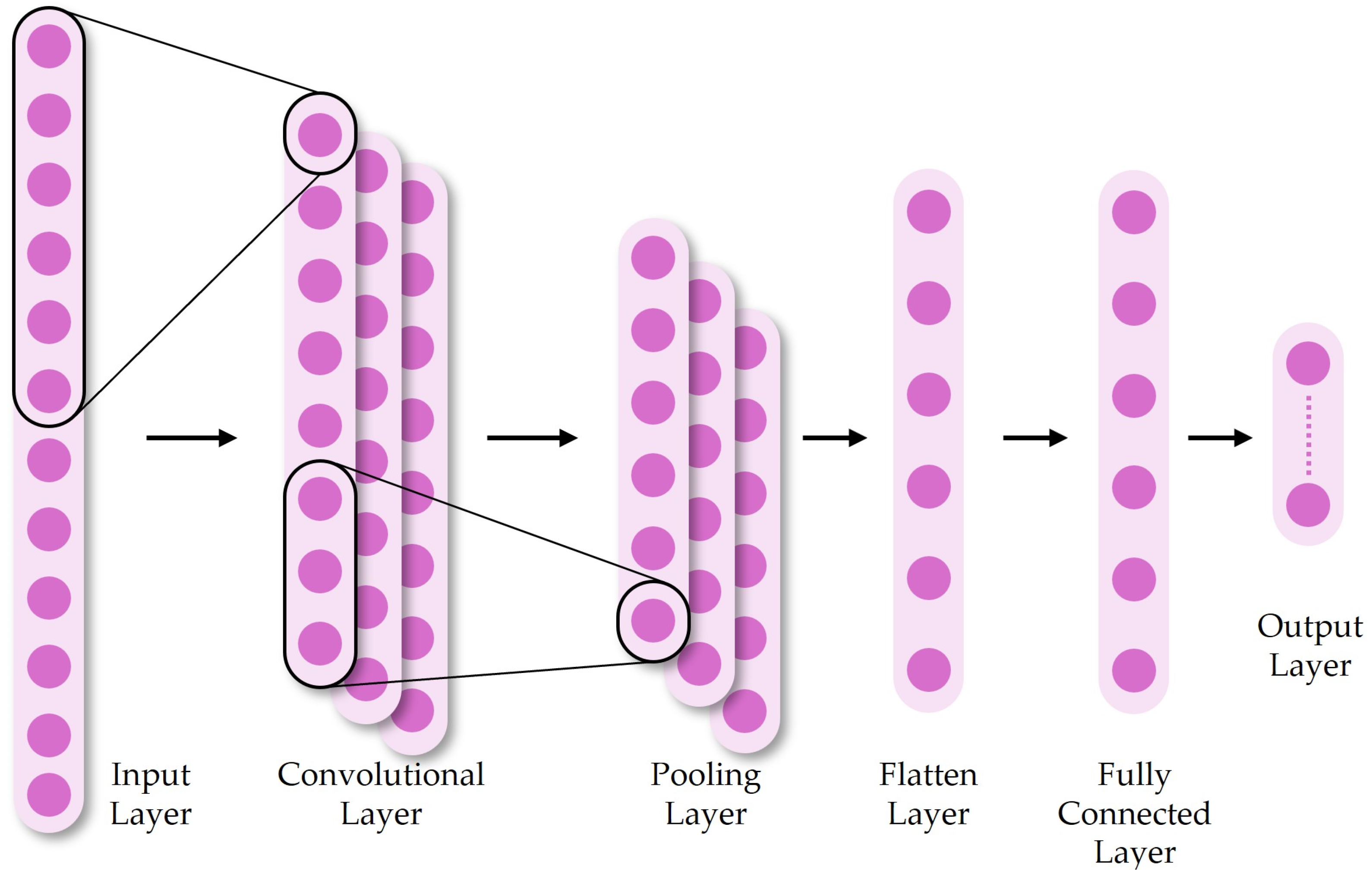
4.2.1. Model Structure and Principle Description (CNN)

In some research cases, researchers usually regard time series as one-dimensional signal input and extract local features through sliding convolution in the time dimension through 1D-CNN. Some researchers also construct multi-site or multi-dimensional data into 2D matrices for 2D convolution, thereby extracting local dependencies in “time and space” at the same time. Figure 9 shows the typical architecture of 1D-CNN in sequence prediction tasks, including convolutional layers, pooling layers, flattening layers, and fully connected layers.

In a 1D-CNN, time series or one-dimensional feature sequences are used as input, and convolutional kernels (filters) slide along this dimension to extract local features. As illustrated, the sequence commences with convolutional and pooling layers, which are subsequently linked to fully connected layers or output layers via a flattening process, facilitating regression or classification tasks. Taking a single-channel input and a single convolutional kernel as an example, Equation (18) presents the convolution operation.

$$z\left[t\right]=\sum _{i=0}^{k-1}w\left[i\right]·x\left[t+1\right]+b$$

(18)

where $x\left[t\right]$ represents the value of the input sequence at position $t$; $k$is the size of the convolutional kernel (filter); $w\left[i\right]$ denotes the weight of the kernel at index$i$; $b$ is the bias term; and $z\left[t\right]$ is the value of the output feature map at position $t$.

For multi-channel input or multiple convolutional kernels, the summation is extended to include weighted sums across channels or kernels, resulting in multiple output channels. In practical networks, activation functions are typically applied immediately after convolution to introduce nonlinearity, as shown in Equation (19):

$$\tilde{z}\left[t\right]=\sigma \left(z\left[t\right]\right)$$

(19)

where $\sigma (\cdot )$ represents the activation function, which enhances the model’s capacity to express nonlinear relationships.

Subsequently, a pooling layer is used to downsample the features (max. pooling or average pooling). This step can effectively reduce the number of parameters and reduce the risk of overfitting while retaining key information. Finally, the output of the convolutional layer is flattened and passed to a fully connected layer or other structure to further integrate and predict sequential features.

In practice, the input data of CNN are usually a multidimensional time series matrix. For 1D-CNN, the input tensor shape is $(N,C)$, where $N$ is the number of data time steps, and $C$ is the feature number corresponding to the pollutant data or meteorological data.

For 2D-CNN, if the spatial distribution of PM_2.5 is considered, the grid data of the air quality monitoring station can be constructed to make the input a tensor of the shape of $(H,W,C)$, similar to image processing. $H$ represents the number of grid rows in PM_2.5 data, $W$ represents the number of grid columns in PM_2.5 data, and $C$ is the number of features.

4.2.2. Research Cases (CNN and Their Hybrid Structures)

Through the successful implementation of various CNN-based research schemes, it has been demonstrated that CNN has advantages in extracting local patterns and performs well in PM_2.5 prediction. Zhang et al., 2021 [175], introduced a method for predicting haze concentration using 1D-CNN for hourly predictions. The input includes haze data for the past 24 h, and the output predicts the concentration level for the next time-step. The prediction accuracy of this method exceeds 95%, which is significantly better than the GRU model and the method achieved an outstanding performance in short-term haze prediction tasks.

In the field of air pollution forecasting, Zheng et al., 2021 [176], developed a random forest-convolutional neural network (RF-CNN) joint model. The model is used for high-resolution PM_2.5 prediction in Delhi and Beijing. In this model, satellite images and meteorological data are used, where the RF component generates a baseline PM_2.5 concentration map, while the CNN component captures spatial residuals to further improve the prediction accuracy. In addition, the model can be applied to the local contrast normalization (LCN) algorithm to automatically detect local PM_2.5 hotspots. The RF-CNN model achieved a normalized RMSE (NRMSE) of ~31% and a normalized MAE (NMAE) of ~19% on a test dataset of two cities. The results showed that the model can effectively detect local changes and hotspot configurations of PM_2.5 concentrations, providing accurate spatial distribution insights for air pollution control.

Unlike 1D-CNN and 2D-CNN, Faraji et al., 2022 [177] introduced a deep learning framework combining a 3D convolutional neural network (3D-CNN) with GRU to predict spatiotemporal PM_2.5 concentrations in urban environments. The model uses Dynamic Time Warping (DTW) to select relevant air quality stations and incorporates meteorological data as auxiliary variables. The experimental results obtained in the Tehran area show that the hourly prediction $R^2$= 0.84 and daily prediction $R^2$ = 0.78 are better than traditional methods such as LSTM, GRU, SVR, and ARIMA.

Kow et al., 2022 [178], introduced an MCNN-BP model that combines a multi-convolutional neural network (MCNN) and a back-propagation neural network (BPNN). The model was used to predict 72 h regional PM_2.5 levels in Taiwan. Atmospheric chemical transport (ACT) model output data and monitoring data were used in the MCNN-BP model, and separate CNNs extracted features from the above datasets. Compared with the single ACT model, the MCNN-BP model significantly reduced the prediction bias and improved the accuracy of spatiotemporal PM_2.5 prediction.

For multi-source data input, Zhu and Xie, 2023 [179] developed a parallel multi-input one-dimensional CNN-BiLSTM (1D-CNN-biLSTM) model for hourly PM_2.5 prediction. The model combines data from the target monitoring station and adjacent monitoring stations, selected according to wind direction and distance, and focuses on seasonal fluctuations. The experimental results show that the average RMSE of the model at nine stations was 3.88, MAE = 2.52, and R² = 0.94, showing a significant improvement in the prediction performance.

Li et al., 2022 [180], designed a hybrid CBAM-CNN-BiLSTM model that combines convolutional block attention module (CBAM), CNN, and BiLSTM for multi-site PM_2.5 prediction in Beijing. The CBAM is used to extract the relationship between pollutants and meteorological data, the CNN architecture is used to capture spatial features, and the BiLSTM architecture can resolve the long-term dependencies of the data. Experimental results show that the model obtained an excellent performance in 1–12 h forecasts and satisfactory results in 13 to 48 h forecasts.

CNN has become an essential tool in PM_2.5 concentration prediction due to its powerful spatial feature extraction capability and flexibility. Still, it has certain limitations in terms of its ability to capture time series features, data quality dependence, and computational cost. Therefore, the current research aims to combine CNN with other deep learning methods and develop more efficient data preprocessing and model optimization techniques.

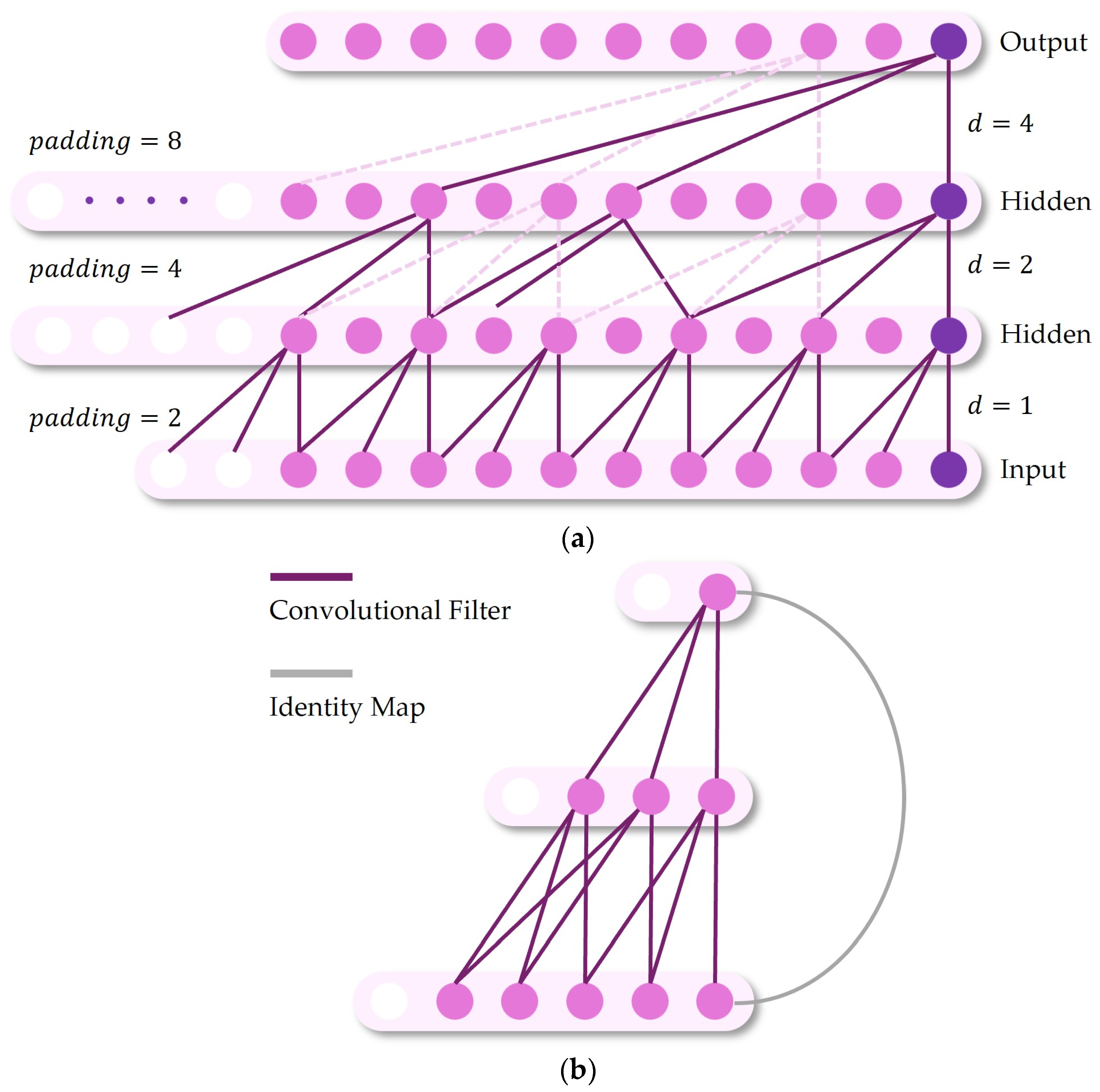
4.3. Temporal Convolutional Network (TCN)

4.3.1. Model Structure and Principle Description (TCN)

TCN [181] is a parallelized structure that has emerged within the domain of time series prediction in recent years. It is based on causal convolution to ensure that information in the direction of time only comes from the past. It uses dilated convolution to capture the dependencies of distant time steps. Compared with RNN/LSTM, TCN can more effectively utilize parallel computing and often shows higher training efficiency in long sequence modeling. Figure 10 shows the overall structure of TCN, the core of which is the combination of multi-layer dilated convolution and skip connections.

As shown in Figure 10, TCN uses different expansion factors in its layers and introduces corresponding degrees of zero padding at the beginning of the input sequence. This design ensures that the output is consistent with the dimension of the input in terms of the time dimension. In the TCN model, as the number of layers increases, the receptive field of the network expands exponentially, enabling it to grasp the long-term dependencies in time series data.

TCN utilizes causal convolution to guarantee that the output at time $t$ is only related to the position in the input sequence that is no greater than $t$, avoiding the leakage of “future information.” If the input sequence is $\{x\left[0\right],x\left[1\right],\dots ,x[T\left]\right\}$, then the causal convolution follows Equation (20) when calculating the output z$\left[t\right]$ (taking a single channel as an example):

$$z\left[t\right]=\sum _{i=0}^{k=1}w\left[i\right]·x\left[t-i\right]+b$$

(20)

where $k$ is the convolution kernel size, $w\left[i\right]$ is the weight of the $i-th$ convolution kernel, and$b$ is the bias term. In order to prevent the output from depending on future moments, the convolution is only performed on $x\left[t-i\right]$, and the output sequence length is ensured to be the same as the input by padding the input sequence with zeros.

In TCN, to cover a longer time range and capture long-distance dependencies, the expansion factor $d$ is introduced so that the convolution kernels are not sampled adjacently on the input sequence. The calculation formula can be written as Equation (21):

$$z\left[t\right]=\sum _{i=0}^{k=1}w\left[i\right]·x\left[t-d·i\right]+b$$

(21)

when $d>1$, the convolution kernel will “skip” $d-1$ positions and take one more point, thereby quickly expanding the receptive field. For example, in the schematic diagram, the first layer ($d=1$) extracts neighboring dependencies, while the second layer ($d=2$) or the third layer ($d=4$) can perceive more distant historical moments.

The actual TCN usually adopts the design of the residual block. After each convolutional layer input $x$ is operated with two (or more) dilated causal convolutions, it is directly incorporated into the initial input to form the output $y$, which is shown in Equation (22):

$$y=x+F(x;W)$$

(22)

where $F ( \cdot ; W )$ represents the convolution transformation function composed of the convolution kernel weight $W$ and the activation function. This residual connection can alleviate the gradient vanishing problem of deep networks and maintain good training results when the number of convolution layers increases. In practice, the input format of TCN is similar to that of 1D-CNN, using the $(N, C)$ structure, but with differences in the convolution method and convolution kernel design.

By parallelizing convolution operations, TCN shows a comparable or better prediction accuracy and training efficiency than LSTM in scenarios such as large-scale time series prediction, especially PM_2.5 multi-step prediction.

4.3.2. Specific Research Cases (TCN)

In recent times, TCN models and hybrid models incorporating TCN elements have gained traction in the realm of PM_2.5 forecasting. Jiang and colleagues, 2021 [182], introduced a hybrid prediction model that combines Complete Ensemble Empirical Mode Decomposition with Adaptive Noise (CEEMDAN) and a Deep Temporal Convolutional Network (DeepTCN) to anticipate PM_2.5 levels in Beijing, China. The study used historical PM_2.5 data, meteorological variables (e.g., temperature, humidity), and time-related features. By decomposing the original data with CEEMDAN and capturing short- and long-term dependencies with DeepTCN, the model significantly improved prediction accuracy and generalization capabilities compared to traditional linear and hybrid models.

Tan et al., 2022 [183], introduced a multi-model ensemble method that combines graph attention network (GAT), LSTM, and TCN and optimized the model through the reinforcement learning (RL-GAT-TCN) method. PM_2.5 concentration data and meteorological data from air quality monitoring stations in multiple cities in China were used in this study. By integrating data from different regions and time scales, this hybrid model effectively captures the spatiotemporal correlation of PM_2.5. The experimental results show that this method outperforms 25 baseline models and exhibits excellent generalization and adaptability.

Lei et al., 2022 [184], designed a multi-channel asymmetric temporal convolutional network (MC-TCN) to predict PM_2.5 concentration in Fushun City, Liaoning Province, China. This study used pollutant concentration data and meteorological parameters collected from 40 air monitoring stations from January to December 2019 as the experimental data. By increasing the number of convolution channels, the model expands its perception range and can grasp additional temporal features. The experimental results show that the MC-TCN model achieves higher levels of prediction accuracy and reliability compared to the base model.

Ren et al., 2023 [185], developed a composite model combining TCN with LSTM for PM_2.5 concentration predictions in Xi’an, China. The dataset used in the study included air quality monitoring data and meteorological parameters from January 2015 to July 2022. The study showed that the R² value of the TCN-LSTM model was always higher than 0.88, significantly outperforming traditional models such as support vector regression and random forest. The key relationships between PM_2.5 and other variables, such as CO, were further identified through a sensitivity analysis, providing valuable insights for environmental monitoring and management.

To address the dual challenges of missing data and prediction in PM_2.5 forecasting, Samal et al., 2024 [186], developed a temporal convolutional network with interpolation blocks (TCN-I). This study used PM_2.5 and meteorological data (temperature, wind speed, humidity) from monitoring stations in India and China. By simultaneously imputing missing values and performing prediction tasks, the TCN-I model outperformed baseline models on multiple datasets, providing a reliable tool for air quality assessment and early warning mechanisms.

Chen et al., 2024 [187], developed a composite model that combines graph convolutional networks (GCNs), TCNs, and autoregressive (AR) components, called GCN-TCN-AR. The model was used to predict PM_2.5 concentrations on the northern slope of the Tianshan Mountains in Xinjiang, China. The study used data from 21 monitoring stations, including PM_2.5 concentrations and meteorological variables (temperature, wind speed, and pressure) in 2019. The model achieved an R² value of more than 0.91 across multiple stations. It also outperformed other neural network models in comparative experiments on accuracy and stability. These findings provide important insights into the spatiotemporal dispersion of PM_2.5, supporting sustainable environmental management in arid regions.

Hu et al., 2024 [188], developed a composite model for predicting PM_2.5 concentration. The model integrates GRU with a modified temporal convolutional network (LR-TCN), referred to as GRU-LR-TCN. In this study, air quality indicators and atmospheric parameters from monitoring stations in many cities in China were used as experimental data. Using RMSE-based weighted integration, the GRU-LR-TCN model showed higher prediction accuracy and adaptability performance on different datasets, demonstrating its utility in predicting high-dimensional temporal data.

TCN-based models can skillfully discern both immediate and extended temporal trends while maintaining computational efficiency due to their parallel computing capabilities. TCNs are often enhanced through hybrid frameworks. These combinations improve model accuracy and generalization by leveraging complementary strengths. In addition, TCN models often incorporate meteorological data and pollutant correlations, further improving prediction performance.

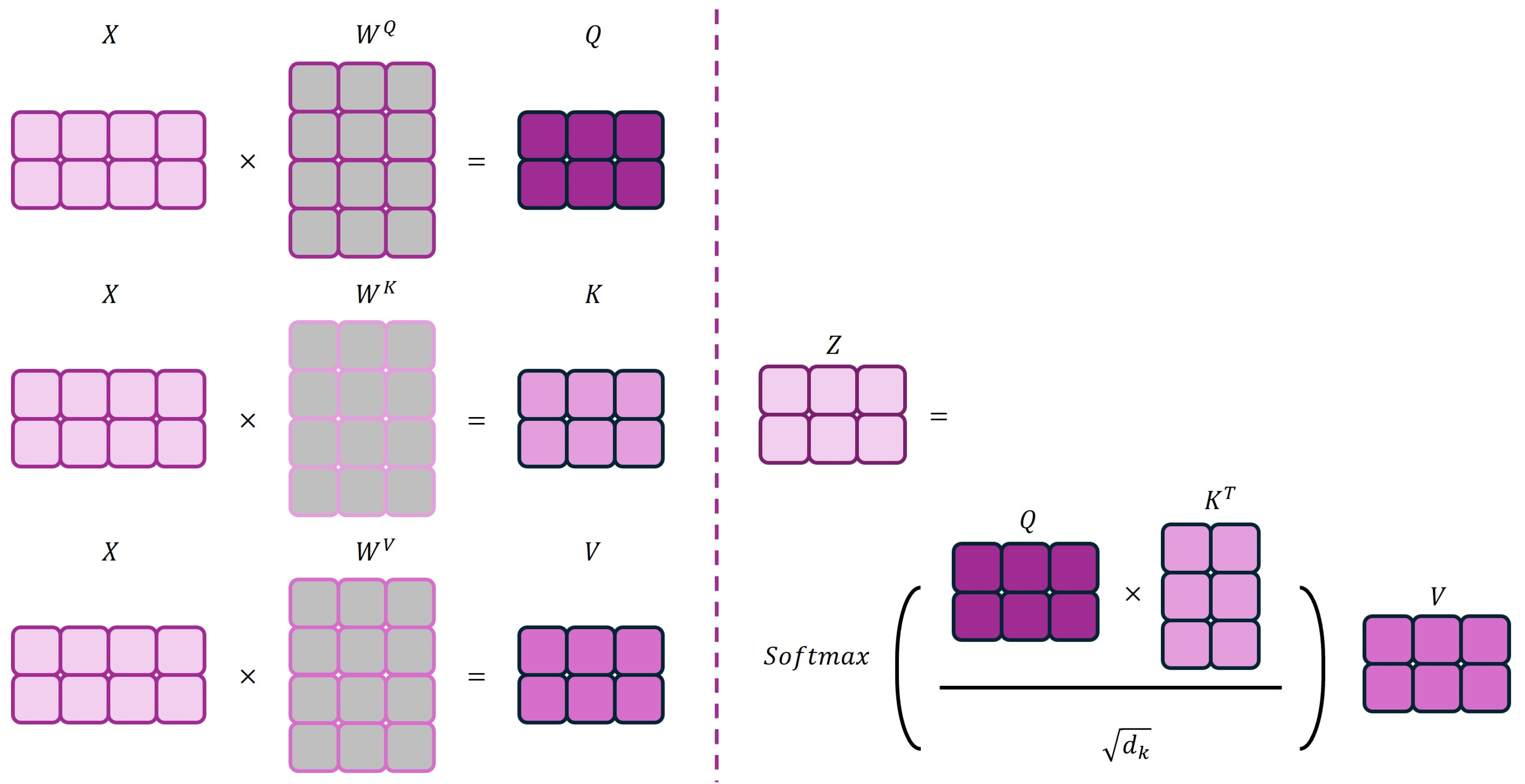
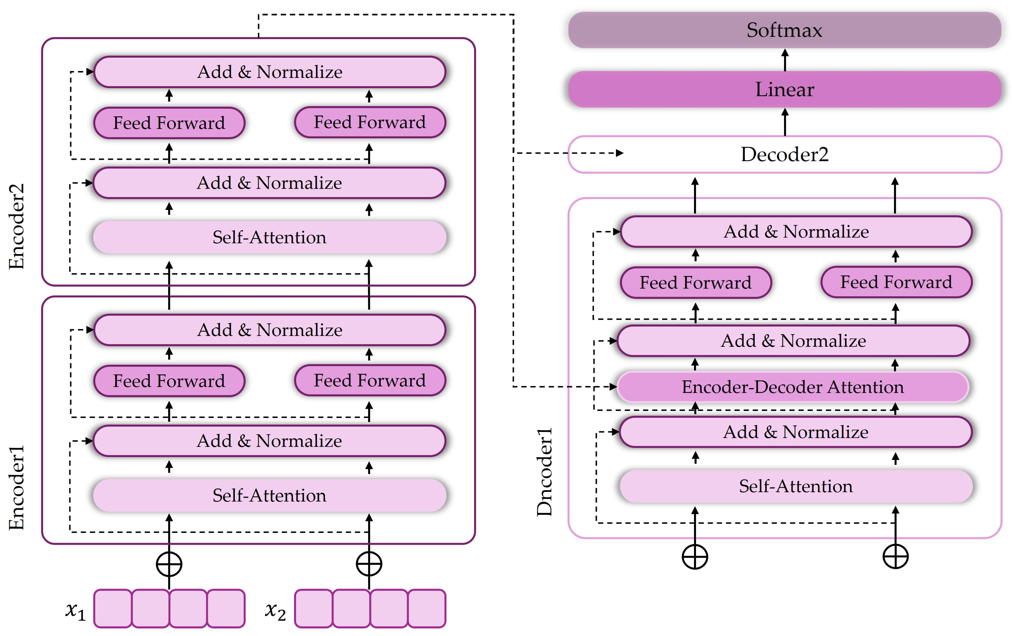
4.4. Transformer and Attention Mechanism

4.4.1. Model Structure and Principle Description (Transformer)

In the PM_2.5 prediction scenario, the Transformer uses a multi-head self-attention mechanism to capture remote dependencies between different time steps or different monitoring sites in parallel, breaking the limitations of RNN on sequence-order calculations. At the same time, Transformer also has flexible scalability in multi-variable and multi-head prediction and can be integrated with multi-source data such as meteorology, traffic, and emissions. Figure 11 shows the Q, K, and V vectors and attention-scoring methods.

In Transformer, the input sequence is first embedded and positionally encoded and then mapped to three sets of vectors: Query (Q), Key (K), and Value (V). As shown in the figure, they are obtained by multiplying the same input $X$ with the trainable parameter matrix $W^Q,W^K,W^V$, shown in Equation (23):

$$Q=X{W}^Q,K=X{W}^K,V=X{W}^V$$

(23)

where $X$ can be a representation of a certain moment or all moments, and $W^Q,W^K,W^V$ are the projection matrices of query, key, and value, respectively. Then, the attention score is calculated as Equation (24):

$$Attention(Q,K,V)=Softmax\left({\displaystyle \frac{Q{K}^T}{\sqrt{d_k}}}\right)V$$

(24)

Among them, $d_k$ represents the vector dimension of $K$ or $Q$, which is used for scaling to prevent the dot product value from being excessively large. The Softmax function normalizes the relevance scores of all moments (or sequence positions) to between 0 and 1 so that the output tensor aggregates the corresponding $V$ information by weight. In the self-attention scenario, $Q=K=V=XW$ (the same input sequence) can capture the dependency between any two positions in the sequence in parallel.

Figure 12 shows a typical Encoder–Decoder structure, with self-attention and feedforward networks in each layer. The input can be an embedded vector of PM_2.5 sequence and other meteorological and traffic characteristics. Transformer distributes dependencies between long-distance time steps or multi-source data by learning attention weights.

In Encoder–Decoder Attention, the Decoder’s Query matrix interacts with the Key and Value generated by the Encoder output to learn cross-module contextual information.

To enhance expressive power and allow the model to capture the dependency patterns in different subspaces, Transformer also splits the above attention mechanism into multi-head calculations, as shown in Equation (25):

$$MultiHead(Q,K,V)=Concat({head}_1,\dots ,{head}_h)W^O$$

(25)

Each ${head}_i=Attention(Q{W}_i^Q,K{W}_i^K,V{W}_i^K)$ uses its own projection matrix, and $Concat$ means concatenating the outputs of all heads in the vector dimension and then multiplying them by $W^O$ for integration. $W^O$ is usually called the Output Projection Matrix. It is learned along with other parameters during model training to coordinate the synergy between the outputs of different attention heads.

The encoder and decoder structures in Figure 13 stack multiple attention and feedforward network modules and use “Add & Normalize” (residual connection + normalization) between layers to maintain stable training. This approach allows the Transformer to process long sequences or multi-dimensional features in parallel. Figure 13 shows the “Add & Normalize” process.

The “Add & Normalize” process aims to convert the input into data with a mean of 0 and a variance of 1 to avoid the input data falling into the saturation area of the activation function.

In practice, the input of Transformer also adopts the $(N, C)$ structure. Because Transformer has no loop structure, position encoding (PE) is required to make the model understand the time order. At this time, the time and pollutant concentration information will form a vector, such as PE (PM_2.5, 12:00), which contains PM_2.5 value + time position information. During the calculation process, the data are converted into the $(K-V-Q)$ form for self-attention calculation. $Q$ represents the information of the current time step (PM_2.5, meteorological variables); $K$ is the information of the historical time step; $V$ is the characteristic value of the historical time step.

Compared with RNN, the most significant advantages of Transformer are parallelization and global dependency capture, which can better cope with the joint prediction needs of multi-variable, multi-site, and long sequences. However, its disadvantage is that the computational cost of the attention matrix increases quadratically with the sequence length, so it is necessary to focus on efficiency or adopt sparse attention improvement in large-scale data scenarios.

4.4.2. Research Cases (Transformer)

Research on Transformer-based air pollutant prediction has also become a hot topic in recent years. Multiple research cases have shown that Transformer can achieve performance advantages over LSTM and CNN when dealing with multidimensional time series forecasts involving multiple pollutants and meteorological elements.

Zeng et al., 2023 [189], introduced a hybrid model that combines the fully integrated empirical mode decomposition adaptive noise (CEEMDAN) with the deep transformer neural network (DeepTransformer) for the PM_2.5 long-term forecasting task. In a specific case, the model is used for long-term PM_2.5 forecasting in China. The model combines a non-autoregressive direct multi-step (DMS) forecasting method with an innovative decoder to improve the prediction accuracy. The experimental results show that DeepTransformer achieves R² = 0.984 and RMSE = 11.61 $\mathsf{\mu }\mathrm{g}/{\mathrm{m}}^3$ in 1 h forecasts and R² = 0.704 and RMSE = 30.78 $\mathsf{\mu }\mathrm{g}/{\mathrm{m}}^3$ in 24 h forecasts. Compared with the single model, this approach significantly improves the prediction accuracy, reducing the MAE and RMSE by 30% and 27%, respectively.

Wang et al., 2023 [190], developed MSAFormer, a Transformer-based model that uses sparse autoencoding and position embedding to predict PM_2.5 concentrations in Haidian District, Beijing. The model can skillfully extract features from high-dimensional meteorological data by integrating the Meteorological Sparse Autoencoding module. The PM_2.5 Prediction Transformer component uses self-attention technology to capture temporal relationships. The experimental results show that it performs well in urban PM_2.5 prediction, an improvement over the traditional method.

Kim et al., 2025 [191], proposed a hybrid attention transformer (HAT) for daily PM_2.5 prediction in Seoul. The experimental results show that the model outperforms traditional chemical transport models (CTMs) and LSTM-based models in terms of prediction accuracy. Compared with CTM, HAT reduces the error by 22.09% and the bias by 82.59%. Notably, the model shows robustness in scenarios such as El Niño events, highlighting its adaptability to dynamic environmental changes.

Al-Qaness et al., 2023 [192], developed the ResInformer model based on the residual transformer. It was used to predict PM_2.5 concentrations in Beijing, Wuhan, and Shijiazhuang. In this case, the ResInformer model used air quality index data collected over 98 months and combined residual blocks to improve computational efficiency. The test results showed that ResInformer outperformed the baseline model in both short-term and long-term predictions, thus demonstrating its effectiveness in urban air quality monitoring.

Zou et al., 2024 [193], developed the PD-LL–Transformer model to predict hourly PM_2.5 concentrations in the Yangtze River Delta urban agglomeration. The model integrated multidimensional embedding, local LSTM, and Transformer blocks, achieving R² = 0.8929 and RMSE = 7.2683 μg/m³ on the 2022 test set. In this case, air pollutant data, meteorological variables, and AOD data derived from the Sunflower 8 satellite were used as experimental data. The test results demonstrated its high accuracy and applicability in regional prediction.

Tong et al., 2024 [194], developed TSPPM25, a spatiotemporal prediction model based on the Transformer architecture, specifically designed for predicting PM_2.5 levels in California. The model uses innovative embedding techniques and a hierarchical attention mechanism to capture the complex spatiotemporal relationships in AOD and the meteorological data. TSPPM25 outperforms LSTM and Bi-LSTM models on multiple evaluation metrics, establishing their robustness in real datasets.

Zhang et al., 2023 [195], proposed a sparse attention transformer network (STN) for PM_2.5 forecasting in Beijing and Taizhou. The model’s design features enable it to reduce computational complexity while maintaining high accuracy. On the Beijing dataset, it achieves R² = 0.937 and RMSE = 19.04 $\mathsf{\mu }\mathrm{g}/{\mathrm{m}}^3$, and on the Taizhou dataset, it achieves R² = 0.924 and RMSE = 5.79 $\mathsf{\mu }\mathrm{g}/{\mathrm{m}}^3$. The model performs well in both short-term and long-term predictions, outperforming baseline models such as Transformer, LSTM, and CNN.

Transformer can effectively model complex temporal and spatial interactions using the self-attention mechanism. The analysis of multiple cases shows that Transformer and its hybrid models outperform traditional methods, such as LSTM and chemical transport models, especially in multi-step and long-term forecasts. Extended and diversified data sources, such as hybrid models, including meteorological data and satellite-derived AOD, further improve their applicability and accuracy. These developments highlight the potential of Transformers as an effective method for predicting air quality and managing public health.

5. Discussion and Future Directions

5.1. Research Status and Main Findings

This survey summarized the preliminary consensus and main findings by systematically sorting out the relevant research on PM_2.5 time series prediction based on deep learning models in recent years. A bibliometric analysis of 2327 articles published between 2014 and 2024 revealed a significant upward trend in PM_2.5 time series forecasting research. The number of publications increased steadily from 2014 to 2021, reflecting the increasing importance of data-driven air quality forecasting. However, there was a slight decline or stagnation in publication output after 2021, indicating that research interest may have stabilized, which may be attributed to research saturation or the maturity of deep learning applications in this field. The keyword co-occurrence analysis highlights the increasing dominance of deep learning-based methods, with models such as CNN, LSTM, and Transformer architectures becoming mainstream methods. Hybrid models that combine deep learning with statistical methods are also gaining popularity, reflecting the need for interpretable and scalable forecasting solutions. Geographically, the research output from China and the United States leads, with strong international collaboration in Europe and Asia. The shift towards interdisciplinary research is evident, with studies increasingly combining meteorological, remote sensing, and socioeconomic data to improve forecast accuracy.

From a technical perspective, first, compared with traditional machine learning or statistical methods, deep learning has shown a stronger ability to capture the complex nonlinear dependencies between PM_2.5 concentrations and various factors. Secondly, the multi-layer neural network structure of the deep learning model provides the possibility of automatically extracting key features from the data, significantly reducing the dependence on artificial feature engineering and showing superior generalization ability when processing complex and large-scale datasets. These advantages show that deep learning has essential application value in the field of PM_2.5 prediction and provides a new research direction for further exploration.

Many studies have shown that combining CNN with hybrid structures such as LSTM can strike a balance between extracting short-term local features and capturing long-range dependencies, thereby showing a relatively stable performance in the multi-step forecasting of PM_2.5 (such as the next 12~48 h). In addition, emerging architectures such as Transformers are friendly to long sequence processing and parallel computing and are gradually becoming strong candidates within the domain of multi-step predicting.

Air pollution prediction often requires integrating multi-source heterogeneous data, which significantly increases the amount of information available in the model and leads to higher requirements for data cleaning, alignment, and preprocessing. Studies that use remote sensing data (AOD) combined with ground monitoring provide a new perspective for capturing large-scale pollution transmission and local emergencies.

The main sources and pollution characteristics of PM_2.5 in different regions vary significantly due to factors such as climate, topography, and industrial structure. This objective factor makes the model prone to performance degradation when generalized across regions. With the complexity of the model structure and the enhancement of computing power, the research content has gradually expanded from predictions at the city scale to regional and even global scales and from general prediction scenarios to diversified applications such as severe pollution emergency responses and public health risk assessments.

Deep learning models are generally regarded as “black boxes”, and the focus on interpreting their predictive outcomes is still in the initial exploration stage. The current research often uses methods such as attention weight visualization and SHAP/LIME to explain the prediction process a posteriori. Still, the principle-level understanding of the pollutant generation mechanism and the cross-temporal and spatial transmission path must be further deepened.

5.2. Existing Problems and Limitations

Although deep learning models are becoming more mature in PM_2.5 prediction, many problems and limitations remain. Among them, data availability and uneven quality are the most critical issues. The data coverage in different regions varies, and many small cities and remote areas lack high-density and high-frequency observation stations. When conducting comparative studies or migrating models across regions, the data scale, monitoring indicators, and quality control standards are inconsistent, and the missing value and noise processing methods are also inconsistent, which affects the overall model performance and comparability.

Although deep models can capture nonlinear mutations to some degree, they still struggle to perceive and accurately quantify sudden events such as sandstorms, fires, and industrial accidents in advance. This requires interdisciplinary integration from prior physical and atmospheric chemical mechanisms, real-time satellite or remote sensing monitoring, and social media information.

Compared with traditional models, deep learning is still weak in theoretical interpretability. For public decision-making and industry applications, the inability to clearly understand the decision-making path and principles within the model may lead to distrust or difficulty in converting the prediction results into a policy-making basis.

The training of long time series and multi-source big data often requires high-performance computing resources, which are costly and require high maintenance pressure. In research scenarios with relatively insufficient computing power or a limited data volume, it is difficult for models to be fully trained or to achieve extrapolated predictions.

5.3. Future Research Directions and Development Trends

Research on PM_2.5 time-series prediction using deep learning techniques holds considerable promise for future development. More diversified data are available with the increasing popularity of new data sources such as mobile sensor networks and social media. In this context, interdisciplinary data fusion is becoming a promising research direction. The use of multi-source data could make a huge potential contribution to improving prediction accuracy and practical applicability. By leveraging flexible platforms to share and align heterogeneous multi-source data, researchers can automate data cleaning and feature extraction to capture the combined effects of a long series, complex geography, and multidimensional socioeconomic factors on PM_2.5 concentrations. At the same time, in pursuit of efficiency and stability for practical applications, modeling methods are no longer limited to traditional architectures. Emerging algorithms, including graph neural networks [196,197,198], reinforcement learning [199,200], and meta-learning [201,202], provide an expanding selection for handling long-term spatiotemporal dependencies, dynamic decision-making, and rapid iteration.

In the process of using deep learning models, interpretability and uncertainty quantification are becoming increasingly important. Public agencies and policymakers need to seek an in-depth understanding of what the model focuses on and the model’s confidence intervals when dealing with pollution events. There are also studies showing that topics on public platforms such as social media have an impact on air pollution control [203]. Mitigating the “black box” nature of deep neural networks is a direction that needs continuous research. In the current research, the visualization of attention weights, post hoc interpretability techniques, or causal inference methods can make the output results more transparent, helping researchers and government agencies better understand the causes of pollution and spatial transmission pathways. In areas lacking comprehensive data, cross-regional transfer learning or federated learning can achieve robust generalization in the presence of significant differences in climate, topography, and emission structures while proposing new data security and privacy protection strategies. At the same time, online learning and data stream-based methods have the potential to capture high-speed data streams and update models in real-time, providing instant air quality alerts in emergencies and winning critical increases in response time.

With the boom in large-scale language models, cross-modal research is facing unprecedented opportunities. Researchers can quickly identify core issues and indicators from the academic literature and policy reports using text-mining and natural language processing technologies. They can also efficiently obtain real-time data from social media and news reports. This multi-source fusion approach provides a broader approach for accurately analyzing the causes of PM_2.5 and opens up new paths for grasping public risk perception.

Furthermore, suppose the language model is combined with meteorological observations, remote sensing monitoring, and socioeconomic data, and the model is calibrated through targeted training. In that case, it can evolve into a comprehensive multimodal analysis tool, gaining deeper insights into fine particulate matter’s formation mechanism and evolution. Strengthening interdisciplinary and cross-departmental collaboration becomes crucial to breaking traditional disciplines’ boundaries, significantly improving the depth and breadth of research and opening up more comprehensive and feasible technical solutions for environmental management and public health protection.

6. Conclusions

This review provides a general overview of the progress of PM_2.5 concentration prediction, focusing on four aspects: bibliometric trends, basic data characteristics, deep learning applications, and future research directions. A systematic bibliometric analysis of journal articles published from 2014 to 2024 demonstrates the growth trend of PM_2.5 time series prediction research activities and the evolution of research hotspots. Through keyword evolution analysis, the research topics transitioned from basic concepts such as “air pollution” to complex methods such as “deep learning” and “neural networks.” This trend reflects the increasing importance of artificial intelligence technology in PM_2.5 prediction.

The study of the physicochemical properties and formation mechanism of PM_2.5 shows that future research directions still need to continuously combine multi-source data. In view of objective problems such as the easy-to-be-true and distorted air pollution data, future research may need to continue developing more appropriate preprocessing techniques to improve reliability and accuracy.

This review combines model architecture and specific cases to widely explore the application of deep learning models in PM_2.5 prediction. These models are good at capturing nonlinear relationships and long-term dynamics. In particular, Transformer is able to effectively model large-scale and long sequence data using its self-attention mechanism and parallel processing capabilities. In all cutting-edge research, models that combine traditional statistical methods with deep learning have significantly improved the accuracy and flexibility of predictions, which may be the direction of future research.

Despite these advances, challenges such as multi-source data integration, model interpretability, and computational resource limitations remain. New technologies such as meta-learning and multi-scale modeling can be explored to improve generalization ability and computational efficiency to address these issues. In addition, embedding prediction models into smart city management platforms can provide real-time monitoring and operational recommendations for decision-makers and the public.

This article summarizes the current status and progress of PM_2.5 prediction research, aiming to provide researchers in this field with resources to quickly obtain the latest progress and trends in this field. At the same time, we hope this survey will provide a systematic introductory guide covering the core content of data acquisition, preprocessing, and model structure.

References

1. Mokhtar, S.B.; Viljoen, J.; van der Kallen, C.J.; Berendschot, T.T.; Dagnelie, P.C.; Albers, J.D.; Soeterboek, J.; Scarpa, F.; Colonna, A.; van der Heide, F.C. Greater exposure to PM2.5 and PM10 was associated with lower corneal nerve measures: The Maastricht study-a cross-sectional study. Environ. Health 2024, 23, 70. [Google Scholar] [CrossRef] [PubMed]
2. Zheng, T.; Wang, Y.; Zhou, Z.; Chen, S.; Jiang, J.; Chen, S. PM2.5 Causes Increased Bacterial Invasion by Affecting HBD1 Expression in the Lung. J. Immunol. Res. 2024, 2024, 6622950. [Google Scholar] [CrossRef]
3. Qiao, H.; Xue, W.T.; Li, L.; Fan, Y.; Xiao, L.; Guo, M.M. Atmospheric Particulate Matter 2.5 (PM2.5) Induces Cell Damage and Pruritus in Human Skin. Biomed. Environ. Sci. 2024, 37, 216–220. [Google Scholar]
4. Li, M.; Tang, B.; Zheng, J.; Luo, W.; Xiong, S.; Ma, Y.; Ren, M.; Yu, Y.; Luo, X.; Mai, B. Typical organic contaminants in hair of adult residents between inland and coastal capital cities in China: Differences in levels and composition profiles, and potential impact factors. Sci. Total Environ. 2023, 869, 161559. [Google Scholar] [CrossRef] [PubMed]
5. Min, K.B.; Min, J.Y. Association of Ambient Particulate Matter Exposure with the Incidence of Glaucoma in Childhood. Am. J. Ophthalmol. 2020, 211, 176–182. [Google Scholar] [CrossRef] [PubMed]
6. Gan, T.; Bambrick, H.; Tong, S.L.; Hu, W.B. Air pollution and liver cancer: A systematic review. J. Environ. Sci. 2023, 126, 817–826. [Google Scholar] [CrossRef]
7. Paik, K.; Na, J.-I.; Huh, C.-H.; Shin, J.-W. Particulate Matter and Its Molecular Effects on Skin: Implications for Various Skin Diseases. Int. J. Mol. Sci. 2024, 25, 9888. [Google Scholar] [CrossRef] [PubMed]
8. Zhang, F.; Zhu, S.; Di, Y.; Pan, M.; Xie, W.; Li, X.; Zhu, W. Ambient PM2.5 components might exacerbate bone loss among middle-aged and elderly women: Evidence from a population-based cross-sectional study. Int. Arch. Occup. Environ. Health 2024, 97, 855–864. [Google Scholar] [CrossRef] [PubMed]
9. Yang, Y.; Li, R.; Cai, M.; Wang, X.J.; Li, H.P.; Wu, Y.L.; Chen, L.; Zou, H.T.; Zhang, Z.L.; Li, H.T.; et al. Ambient air pollution, bone mineral density and osteoporosis: Results from a national population-based cohort study. Chemosphere 2023, 310, 8. [Google Scholar] [CrossRef]
10. Jiang, R.; Qu, Q.; Wang, Z.; Luo, F.; Mou, S. Association between air pollution and bone mineral density: A Mendelian randomization study. Arch. Med. Sci. 2024, 20, 1334–1338. [Google Scholar] [CrossRef]
11. Zhao, L.; Li, Z.; Qu, L. A novel machine learning-based artificial intelligence method for predicting the air pollution index PM2.5. J. Clean. Prod. 2024, 468, 143042. [Google Scholar] [CrossRef]
12. Xiao, Y.-j.; Wang, X.-k.; Wang, J.-q.; Zhang, H.-y. An adaptive decomposition and ensemble model for short-term air pollutant concentration forecast using ICEEMDAN-ICA. Technol. Forecast. Soc. Change 2021, 166, 120655. [Google Scholar] [CrossRef]
13. Liao, K.; Huang, X.; Dang, H.; Ren, Y.; Zuo, S.; Duan, C. Statistical Approaches for Forecasting Primary Air Pollutants: A Review. Atmosphere 2021, 12, 686. [Google Scholar] [CrossRef]
14. Zhang, B.; Rong, Y.; Yong, R.; Qin, D.; Li, M.; Zou, G.; Pan, J. Deep learning for air pollutant concentration prediction: A review. Atmos. Environ. 2022, 290, 119347. [Google Scholar] [CrossRef]
15. Su, J.G.; Meng, Y.-Y.; Chen, X.; Molitor, J.; Yue, D.; Jerrett, M. Predicting differential improvements in annual pollutant concentrations and exposures for regulatory policy assessment. Environ. Int. 2020, 143, 105942. [Google Scholar] [CrossRef] [PubMed]
16. Wen, Q.; Zhang, T. Economic policy uncertainty and industrial pollution: The role of environmental supervision by local governments. China Econ. Rev. 2022, 71, 101723. [Google Scholar] [CrossRef]
17. Yang, W.; Wang, J.; Zhang, K.; Hao, Y. A novel air pollution forecasting, health effects, and economic cost assessment system for environmental management: From a new perspective of the district-level. J. Clean. Prod. 2023, 417, 138027. [Google Scholar] [CrossRef]
18. Wong, K.-S.; Chew, Y.J.; Ooi, S.Y.; Pang, Y.H. Toward forecasting future day air pollutant index in Malaysia. J. Supercomput. 2021, 77, 4813–4830. [Google Scholar] [CrossRef]
19. Li, H.; Xu, X.-L.; Dai, D.-W.; Huang, Z.-Y.; Ma, Z.; Guan, Y.-J. Air pollution and temperature are associated with increased COVID-19 incidence: A time series study. Int. J. Infect. Dis. 2020, 97, 278–282. [Google Scholar] [CrossRef]
20. Gu, J.; Shi, Y.; Zhu, Y.; Chen, N.; Wang, H.; Zhang, Z.; Chen, T. Ambient air pollution and cause-specific risk of hospital admission in China: A nationwide time-series study. PLoS Med. 2020, 17, e1003188. [Google Scholar] [CrossRef] [PubMed]
21. Moshammer, H.; Poteser, M.; Hutter, H.-P. COVID-19 and air pollution in Vienna—A time series approach. Wien. Klin. Wochenschr. 2021, 133, 951–957. [Google Scholar] [CrossRef] [PubMed]
22. Kim, H.; Lee, J.-T. Inter-mortality displacement hypothesis and short-term effect of ambient air pollution on mortality in seven major cities of South Korea: A time-series analysis. Int. J. Epidemiol. 2020, 49, 1802–1812. [Google Scholar] [CrossRef] [PubMed]
23. He, Z.; Liu, P.; Zhao, X.; He, X.; Liu, J.; Mu, Y. Responses of surface O3 and PM2.5 trends to changes of anthropogenic emissions in summer over Beijing during 2014–2019: A study based on multiple linear regression and WRF-Chem. Sci. Total Environ. 2022, 807, 150792. [Google Scholar] [CrossRef]
24. Wong, P.-Y.; Lee, H.-Y.; Chen, Y.-C.; Zeng, Y.-T.; Chern, Y.-R.; Chen, N.-T.; Candice Lung, S.-C.; Su, H.-J.; Wu, C.-D. Using a land use regression model with machine learning to estimate ground level PM2.5. Environ. Pollut. 2021, 277, 116846. [Google Scholar] [CrossRef] [PubMed]
25. Kumar, V.; Sahu, M. Evaluation of nine machine learning regression algorithms for calibration of low-cost PM2.5 sensor. J. Aerosol Sci. 2021, 157, 105809. [Google Scholar] [CrossRef]
26. Zhang, P.; Ma, W.; Wen, F.; Liu, L.; Yang, L.; Song, J.; Wang, N.; Liu, Q. Estimating PM2.5 concentration using the machine learning GA-SVM method to improve the land use regression model in Shaanxi, China. Ecotoxicol. Environ. Saf. 2021, 225, 112772. [Google Scholar] [CrossRef]
27. Ibrir, A.; Kerchich, Y.; Hadidi, N.; Merabet, H.; Hentabli, M. Prediction of the concentrations of PM1, PM2.5, PM4, and PM10 by using the hybrid dragonfly-SVM algorithm. Air Qual. Atmos. Health 2021, 14, 313–323. [Google Scholar] [CrossRef]
28. Lai, X.; Li, H.; Pan, Y. A combined model based on feature selection and support vector machine for PM2.5 prediction. J. Intell. Fuzzy Syst. 2021, 40, 10099–10113. [Google Scholar] [CrossRef]
29. Sethi, J.K.; Mittal, M. Efficient weighted naive bayes classifiers to predict air quality index. Earth Sci. Inform. 2022, 15, 541–552. [Google Scholar] [CrossRef]
30. Apriani, N.F.; Salampessy, J.E.B.; Kusumadewi, S.; Rizky, R.R.; Siagian, A.H.A.M.; Siahaan, F.B.; Riyanto, S.; Sriyadi; Irfiani, E. Classification and Forecasting Air Pollution Using Naive Bayes and Prophet: A Use Case of Air Quality Index in Jakarta. In Proceedings of the 2024 International Conference on Computer, Control, Informatics and its Applications (IC3INA), Bandung, Indonesia, 9–10 October 2024; pp. 279–284. [Google Scholar]
31. Merdani, A. Comparative Machine Learning Analysis of PM25 and PM10 Forecasting in Albania. In Proceedings of the 2024 International Conference on Software, Telecommunications and Computer Networks (SoftCOM), Croatia, Balkans, 26–28 September 2024; pp. 1–7. [Google Scholar]
32. Guo, B.; Zhang, D.; Pei, L.; Su, Y.; Wang, X.; Bian, Y.; Zhang, D.; Yao, W.; Zhou, Z.; Guo, L. Estimating PM2.5 concentrations via random forest method using satellite, auxiliary, and ground-level station dataset at multiple temporal scales across China in 2017. Sci. Total Environ. 2021, 778, 146288. [Google Scholar] [CrossRef]
33. Su, Z.; Lin, L.; Chen, Y.; Hu, H. Understanding the distribution and drivers of PM2.5 concentrations in the Yangtze River Delta from 2015 to 2020 using Random Forest Regression. Environ. Monit. Assess. 2022, 194, 284. [Google Scholar] [CrossRef] [PubMed]
34. Zhang, Y.; Zhai, S.; Huang, J.; Li, X.; Wang, W.; Zhang, T.; Yin, F.; Ma, Y. Estimating high-resolution PM2.5 concentration in the Sichuan Basin using a random forest model with data-driven spatial autocorrelation terms. J. Clean. Prod. 2022, 380, 134890. [Google Scholar] [CrossRef]
35. Zhang, T.; He, W.; Zheng, H.; Cui, Y.; Song, H.; Fu, S. Satellite-based ground PM2.5 estimation using a gradient boosting decision tree. Chemosphere 2021, 268, 128801. [Google Scholar] [CrossRef]
36. Liu, M.; Chen, H.; Wei, D.; Wu, Y.; Li, C. Nonlinear relationship between urban form and street-level PM2.5 and CO based on mobile measurements and gradient boosting decision tree models. Build. Environ. 2021, 205, 108265. [Google Scholar] [CrossRef]
37. Wang, Z.; Wu, X.; Wu, Y. A spatiotemporal XGBoost model for PM2.5 concentration prediction and its application in Shanghai. Heliyon 2023, 9, e22569. [Google Scholar] [CrossRef]
38. Jeong, J.I.; Park, R.J.; Yeh, S.-W.; Roh, J.-W. Statistical predictability of wintertime PM2.5 concentrations over East Asia using simple linear regression. Sci. Total Environ. 2021, 776, 146059. [Google Scholar] [CrossRef]
39. Gong, H.; Guo, J.; Mu, Y.; Guo, Y.; Hu, T.; Li, S.; Luo, T.; Sun, Y. Atmospheric PM2.5 Prediction Model Based on Principal Component Analysis and SSA–SVM. Sustainability 2024, 16, 832. [Google Scholar] [CrossRef]
40. Tella, A.; Balogun, A.-L.; Adebisi, N.; Abdullah, S. Spatial assessment of PM10 hotspots using Random Forest, K-Nearest Neighbour and Naïve Bayes. Atmos. Pollut. Res. 2021, 12, 101202. [Google Scholar] [CrossRef]
41. Chen, C.-C.; Wang, Y.-R.; Yeh, H.-Y.; Lin, T.-H.; Huang, C.-S.; Wu, C.-F. Estimating monthly PM2.5 concentrations from satellite remote sensing data, meteorological variables, and land use data using ensemble statistical modeling and a random forest approach. Environ. Pollut. 2021, 291, 118159. [Google Scholar] [CrossRef]
42. He, W.; Meng, H.; Han, J.; Zhou, G.; Zheng, H.; Zhang, S. Spatiotemporal PM2.5 estimations in China from 2015 to 2020 using an improved gradient boosting decision tree. Chemosphere 2022, 296, 134003. [Google Scholar] [CrossRef] [PubMed]
43. Unik, M.; Sitanggang, I.S.; Syaufina, L.; Jaya, I.N.S. PM2.5 estimation using machine learning models and satellite data: A literature review. Int. J. Adv. Comput. Sci. Appl. 2023, 14, 359–370. [Google Scholar] [CrossRef]
44. Torres, J.F.; Hadjout, D.; Sebaa, A.; Martínez-Álvarez, F.; Troncoso, A. Deep Learning for Time Series Forecasting: A Survey. Big Data 2020, 9, 3–21. [Google Scholar] [CrossRef]
45. Lim, B.; Zohren, S. Time-series forecasting with deep learning: A survey. Philos. Trans. R. Soc. A 2021, 379, 20200209. [Google Scholar] [CrossRef]
46. Park, Y.; Kwon, B.; Heo, J.; Hu, X.; Liu, Y.; Moon, T. Estimating PM2.5 concentration of the conterminous United States via interpretable convolutional neural networks. Environ. Pollut. 2020, 256, 113395. [Google Scholar] [CrossRef] [PubMed]
47. Xia, S.; Zhang, R.; Zhang, L.; Wang, T.; Wang, W. Multi-dimensional distribution prediction of PM2.5 concentration in urban residential areas based on CNN. Build. Environ. 2025, 267, 112167. [Google Scholar] [CrossRef]
48. Kow, P.-Y.; Wang, Y.-S.; Zhou, Y.; Kao, I.F.; Issermann, M.; Chang, L.-C.; Chang, F.-J. Seamless integration of convolutional and back-propagation neural networks for regional multi-step-ahead PM2.5 forecasting. J. Clean. Prod. 2020, 261, 121285. [Google Scholar] [CrossRef]
49. Dai, X.; Liu, J.; Li, Y. A recurrent neural network using historical data to predict time series indoor PM2.5 concentrations for residential buildings. Indoor Air 2021, 31, 1228–1237. [Google Scholar] [CrossRef] [PubMed]
50. Liu, B.; Yan, S.; Li, J.; Li, Y.; Lang, J.; Qu, G. A Spatiotemporal Recurrent Neural Network for Prediction of Atmospheric PM2.5: A Case Study of Beijing. IEEE Trans. Comput. Soc. Syst. 2021, 8, 578–588. [Google Scholar] [CrossRef]
51. Xie, N.; Li, B. PM2.5 Monitoring and Prediction Based on IOT and RNN Neural Network. In Proceedings of the Artificial Intelligence Security and Privacy, Singapore, 6–7 December 2024; pp. 241–253. [Google Scholar]
52. Gao, X.; Li, W. A graph-based LSTM model for PM2.5 forecasting. Atmos. Pollut. Res. 2021, 12, 101150. [Google Scholar] [CrossRef]
53. Kristiani, E.; Lin, H.; Lin, J.-R.; Chuang, Y.-H.; Huang, C.-Y.; Yang, C.-T. Short-Term Prediction of PM2.5 Using LSTM Deep Learning Methods. Sustainability 2022, 14, 2068. [Google Scholar] [CrossRef]
54. Lin, M.-D.; Liu, P.-Y.; Huang, C.-W.; Lin, Y.-H. The application of strategy based on LSTM for the short-term prediction of PM2.5 in city. Sci. Total Environ. 2024, 906, 167892. [Google Scholar] [CrossRef] [PubMed]
55. Huang, G.; Li, X.; Zhang, B.; Ren, J. PM2.5 concentration forecasting at surface monitoring sites using GRU neural network based on empirical mode decomposition. Sci. Total Environ. 2021, 768, 144516. [Google Scholar] [CrossRef] [PubMed]
56. Qing, L. PM2.5 Concentration Prediction Using GRA-GRU Network in Air Monitoring. Sustainability 2023, 15, 1973. [Google Scholar] [CrossRef]
57. Jiang, W.; Li, S.; Xie, Z.; Chen, W.; Zhan, C. Short-term PM2.5 Forecasting with a Hybrid Model Based on Ensemble GRU Neural Network. In Proceedings of the 2020 IEEE 18th International Conference on Industrial Informatics (INDIN), Warwick, UK, 20–23 July 2020; pp. 729–733. [Google Scholar]
58. Yu, M.; Masrur, A.; Blaszczak-Boxe, C. Predicting hourly PM2.5 concentrations in wildfire-prone areas using a SpatioTemporal Transformer model. Sci. Total Environ. 2023, 860, 160446. [Google Scholar] [CrossRef]
59. Cui, B.; Liu, M.; Li, S.; Jin, Z.; Zeng, Y.; Lin, X. Deep learning methods for atmospheric PM2.5 prediction: A comparative study of transformer and CNN-LSTM-attention. Atmos. Pollut. Res. 2023, 14, 101833. [Google Scholar] [CrossRef]
60. Dai, Z.; Ren, G.; Jin, Y.; Zhang, J. Research on PM2.5 concentration prediction based on transformer. J. Phys. Conf. Ser. 2024, 2813, 012023. [Google Scholar] [CrossRef]
61. Wang, P.; Zhang, H.; Qin, Z.; Zhang, G. A novel hybrid-Garch model based on ARIMA and SVM for PM2.5 concentrations forecasting. Atmos. Pollut. Res. 2017, 8, 850–860. [Google Scholar] [CrossRef]
62. Pakrooh, P.; Pishbahar, E. Forecasting Air Pollution Concentrations in Iran, Using a Hybrid Model. Pollution 2019, 5, 739–747. [Google Scholar] [CrossRef]
63. Liu, B.; Jin, Y.; Li, C. Analysis and prediction of air quality in Nanjing from autumn 2018 to summer 2019 using PCR–SVR–ARMA combined model. Sci. Rep. 2021, 11, 348. [Google Scholar] [CrossRef] [PubMed]
64. Shahriar, S.A.; Kayes, I.; Hasan, K.; Hasan, M.; Islam, R.; Awang, N.R.; Hamzah, Z.; Rak, A.E.; Salam, M.A. Potential of ARIMA-ANN, ARIMA-SVM, DT and CatBoost for Atmospheric PM2.5 Forecasting in Bangladesh. Atmosphere 2021, 12, 100. [Google Scholar] [CrossRef]
65. Chen, C. CiteSpace: A Practical Guide for Mapping Scientific Literature; Nova Science Publishers: Hauppauge, NY, USA, 2016. [Google Scholar]
66. Tucker, W.G. An overview of PM2.5 sources and control strategies. Fuel Process. Technol. 2000, 65–66, 379–392. [Google Scholar] [CrossRef]
67. Lim, C.-H.; Ryu, J.; Choi, Y.; Jeon, S.W.; Lee, W.-K. Understanding global PM2.5 concentrations and their drivers in recent decades (1998–2016). Environ. Int. 2020, 144, 106011. [Google Scholar] [CrossRef]
68. Burke, M.; Childs, M.L.; de la Cuesta, B.; Qiu, M.; Li, J.; Gould, C.F.; Heft-Neal, S.; Wara, M. The contribution of wildfire to PM2.5 trends in the USA. Nature 2023, 622, 761–766. [Google Scholar] [CrossRef] [PubMed]
69. Geng, G.; Xiao, Q.; Liu, S.; Liu, X.; Cheng, J.; Zheng, Y.; Xue, T.; Tong, D.; Zheng, B.; Peng, Y.; et al. Tracking Air Pollution in China: Near Real-Time PM2.5 Retrievals from Multisource Data Fusion. Environ. Sci. Technol. 2021, 55, 12106–12115. [Google Scholar] [CrossRef]
70. Pan, S.; Qiu, Y.; Li, M.; Yang, Z.; Liang, D. Recent Developments in the Determination of PM2.5 Chemical Composition. Bull. Environ. Contam. Toxicol. 2022, 108, 819–823. [Google Scholar] [CrossRef]
71. Alves, C.; Evtyugina, M.; Vicente, E.; Vicente, A.; Rienda, I.C.; de la Campa, A.S.; Tomé, M.; Duarte, I. PM2.5 chemical composition and health risks by inhalation near a chemical complex. J. Environ. Sci. 2023, 124, 860–874. [Google Scholar] [CrossRef] [PubMed]
72. Sidwell, A.; Smith, S.C.; Roper, C. A comparison of fine particulate matter (PM2.5) in vivo exposure studies incorporating chemical analysis. J. Toxicol. Environ. Health Part B 2022, 25, 422–444. [Google Scholar] [CrossRef]
73. Kim, N.K.; Kim, Y.P.; Ghim, Y.S.; Song, M.J.; Kim, C.H.; Jang, K.S.; Lee, K.Y.; Shin, H.J.; Jung, J.S.; Wu, Z.; et al. Spatial distribution of PM2.5 chemical components during winter at five sites in Northeast Asia: High temporal resolution measurement study. Atmos. Environ. 2022, 290, 119359. [Google Scholar] [CrossRef]
74. Xie, Y.; Zhou, M.; Hunt, K.M.R.; Mauzerall, D.L. Recent PM2.5 air quality improvements in India benefited from meteorological variation. Nat. Sustain. 2024, 7, 983–993. [Google Scholar] [CrossRef]
75. Zhang, X.; Xu, H.; Liang, D. Spatiotemporal variations and connections of single and multiple meteorological factors on PM2.5 concentrations in Xi’an, China. Atmos. Environ. 2022, 275, 119015. [Google Scholar] [CrossRef]
76. Lu, X.; Yuan, D.; Chen, Y.; Fung, J.C.H. Impacts of urbanization and long-term meteorological variations on global PM2.5 and its associated health burden. Environ. Pollut. 2021, 270, 116003. [Google Scholar] [CrossRef] [PubMed]
77. Liu, G.; Dong, X.; Kong, Z.; Dong, K. Does national air quality monitoring reduce local air pollution? The case of PM2.5 for China. J. Environ. Manag. 2021, 296, 113232. [Google Scholar] [CrossRef]
78. Liu, S.; Geng, G.; Xiao, Q.; Zheng, Y.; Liu, X.; Cheng, J.; Zhang, Q. Tracking Daily Concentrations of PM2.5 Chemical Composition in China since 2000. Environ. Sci. Technol. 2022, 56, 16517–16527. [Google Scholar] [CrossRef]
79. Zhang, Q.; Zheng, Y.; Tong, D.; Shao, M.; Wang, S.; Zhang, Y.; Xu, X.; Wang, J.; He, H.; Liu, W.; et al. Drivers of improved PM2.5 air quality in China from 2013 to 2017. Proc. Natl. Acad. Sci. USA 2019, 116, 24463–24469. [Google Scholar] [CrossRef] [PubMed]
80. Solomon, P.A.; Crumpler, D.; Flanagan, J.B.; Jayanty, R.K.M.; Rickman, E.E.; McDade, C.E. U.S. National PM2.5 Chemical Speciation Monitoring Networks—CSN and IMPROVE: Description of networks. J. Air Waste Manag. Assoc. 2014, 64, 1410–1438. [Google Scholar] [CrossRef]
81. Heo, J.; Adams, P.J.; Gao, H.O. Public Health Costs of Primary PM2.5 and Inorganic PM2.5 Precursor Emissions in the United States. Environ. Sci. Technol. 2016, 50, 6061–6070. [Google Scholar] [CrossRef]
82. Nazarenko, Y.; Pal, D.; Ariya, P.A. Air quality standards for the concentration of particulate matter 2.5, global descriptive analysis. Bull World Health Organ 2021, 99, 125–137d. [Google Scholar] [CrossRef] [PubMed]
83. Bailie, C.R.; Ghosh, J.K.C.; Kirk, M.D.; Sullivan, S.G. Effect of ambient PM2.5 on healthcare utilisation for acute respiratory illness, Melbourne, Victoria, Australia, 2014-2019. J. Air Waste Manag. Assoc. 2023, 73, 120–132. [Google Scholar] [CrossRef]
84. Chang, L.T.-C.; Scorgie, Y.; Duc, H.N.; Monk, K.; Fuchs, D.; Trieu, T. Major Source Contributions to Ambient PM2.5 and Exposures within the New South Wales Greater Metropolitan Region. Atmosphere 2019, 10, 138. [Google Scholar] [CrossRef]
85. Danesi, N.; Jain, M.; Lee, Y.H.; Dev, S. Predicting Ground-based PM2.5 Concentration in Queensland, Australia. In Proceedings of the 2021 Photonics & Electromagnetics Research Symposium (PIERS), Hangzhou, China, 21–25 November 2021; pp. 1183–1190. [Google Scholar]
86. Dong, T.T.T.; Stock, W.D.; Callan, A.C.; Strandberg, B.; Hinwood, A.L. Emission factors and composition of PM2.5 from laboratory combustion of five Western Australian vegetation types. Sci. Total Environ. 2020, 703, 134796. [Google Scholar] [CrossRef]
87. Johnston, F.H.; Borchers-Arriagada, N.; Morgan, G.G.; Jalaludin, B.; Palmer, A.J.; Williamson, G.J.; Bowman, D.M.J.S. Unprecedented health costs of smoke-related PM2.5 from the 2019–2020 Australian megafires. Nat. Sustain. 2021, 4, 42–47. [Google Scholar] [CrossRef]
88. Kumar, N.; Park, R.J.; Jeong, J.I.; Woo, J.-H.; Kim, Y.; Johnson, J.; Yarwood, G.; Kang, S.; Chun, S.; Knipping, E. Contributions of international sources to PM2.5 in South Korea. Atmos. Environ. 2021, 261, 118542. [Google Scholar] [CrossRef]
89. Kumar, N.; Johnson, J.; Yarwood, G.; Woo, J.-H.; Kim, Y.; Park, R.J.; Jeong, J.I.; Kang, S.; Chun, S.; Knipping, E. Contributions of domestic sources to PM2.5 in South Korea. Atmos. Environ. 2022, 287, 119273. [Google Scholar] [CrossRef]
90. Lee, H.-M.; Kim, N.K.; Ahn, J.; Park, S.-M.; Lee, J.Y.; Kim, Y.P. When and why PM2.5 is high in Seoul, South Korea: Interpreting long-term (2015–2021) ground observations using machine learning and a chemical transport model. Sci. Total Environ. 2024, 920, 170822. [Google Scholar] [CrossRef]
91. Cesari, D.; De Benedetto, G.E.; Bonasoni, P.; Busetto, M.; Dinoi, A.; Merico, E.; Chirizzi, D.; Cristofanelli, P.; Donateo, A.; Grasso, F.M.; et al. Seasonal variability of PM2.5 and PM10 composition and sources in an urban background site in Southern Italy. Sci. Total Environ. 2018, 612, 202–213. [Google Scholar] [CrossRef]
92. Ciucci, A.; D’Elia, I.; Wagner, F.; Sander, R.; Ciancarella, L.; Zanini, G.; Schöpp, W. Cost-effective reductions of PM2.5 concentrations and exposure in Italy. Atmos. Environ. 2016, 140, 84–93. [Google Scholar] [CrossRef]
93. Stafoggia, M.; Bellander, T.; Bucci, S.; Davoli, M.; de Hoogh, K.; de’ Donato, F.; Gariazzo, C.; Lyapustin, A.; Michelozzi, P.; Renzi, M.; et al. Estimation of daily PM10 and PM2.5 concentrations in Italy, 2013–2015, using a spatiotemporal land-use random-forest model. Environ. Int. 2019, 124, 170–179. [Google Scholar] [CrossRef]
94. Peng, S.; Ding, Y.; Liu, W.; Li, Z. 1 km monthly temperature and precipitation dataset for China from 1901 to 2017. Earth Syst. Sci. Data 2019, 11, 1931–1946. [Google Scholar] [CrossRef]
95. He, J.; Yang, K.; Tang, W.; Lu, H.; Qin, J.; Chen, Y.; Li, X. The first high-resolution meteorological forcing dataset for land process studies over China. Sci. Data 2020, 7, 25. [Google Scholar] [CrossRef] [PubMed]
96. Zhang, X.; Xu, X.; Ding, Y.; Liu, Y.; Zhang, H.; Wang, Y.; Zhong, J. The impact of meteorological changes from 2013 to 2017 on PM2.5 mass reduction in key regions in China. Sci. China Earth Sci. 2019, 62, 1885–1902. [Google Scholar] [CrossRef]
97. Banzon, V.; Smith, T.M.; Chin, T.M.; Liu, C.; Hankins, W. A long-term record of blended satellite and in situ sea-surface temperature for climate monitoring, modeling and environmental studies. Earth Syst. Sci. Data 2016, 8, 165–176. [Google Scholar] [CrossRef]
98. Young, A.M.; Skelly, K.T.; Cordeira, J.M. High-impact hydrologic events and atmospheric rivers in California: An investigation using the NCEI Storm Events Database. Geophys. Res. Lett. 2017, 44, 3393–3401. [Google Scholar] [CrossRef]
99. Brewer, M.J.; Hollingshead, A.; Dissen, J.; Jones, N.; Webster, L.F. User Needs for Weather and Climate Information: 2019 NCEI Users’ Conference. Bull. Am. Meteorol. Soc. 2020, 101, E645–E649. [Google Scholar] [CrossRef]
100. Su, C.H.; Eizenberg, N.; Steinle, P.; Jakob, D.; Fox-Hughes, P.; White, C.J.; Rennie, S.; Franklin, C.; Dharssi, I.; Zhu, H. BARRA v1.0: The Bureau of Meteorology Atmospheric high-resolution Regional Reanalysis for Australia. Geosci. Model Dev. 2019, 12, 2049–2068. [Google Scholar] [CrossRef]
101. Hudson, D.; Alves, O.; Hendon, H.H.; Lim, E.-P.; Liu, G.; Luo, J.-J.; MacLachlan, C.; Marshall, A.G.; Shi, L.; Wang, G.; et al. ACCESS-S1 The new Bureau of Meteorology multi-week to seasonal prediction system. J. South. Hemisph. Earth Syst. Sci. 2017, 67, 132–159. [Google Scholar] [CrossRef]
102. Park, M.S.; Park, S.H.; Chae, J.H.; Choi, M.H.; Song, Y.; Kang, M.; Roh, J.W. High-resolution urban observation network for user-specific meteorological information service in the Seoul Metropolitan Area, South Korea. Atmos. Meas. Tech. 2017, 10, 1575–1594. [Google Scholar] [CrossRef]
103. Park, M.-S. Overview of Meteorological Surface Variables and Boundary-layer Structures in the Seoul Metropolitan Area during the MAPS-Seoul Campaign. Aerosol Air Qual. Res. 2018, 18, 2157–2172. [Google Scholar] [CrossRef]
104. Hong, S.-Y.; Kwon, Y.C.; Kim, T.-H.; Esther Kim, J.-E.; Choi, S.-J.; Kwon, I.-H.; Kim, J.; Lee, E.-H.; Park, R.-S.; Kim, D.-I. The Korean Integrated Model (KIM) System for Global Weather Forecasting. Asia-Pac. J. Atmos. Sci. 2018, 54, 267–292. [Google Scholar] [CrossRef]
105. Panagos, P.; Ballabio, C.; Borrelli, P.; Meusburger, K.; Klik, A.; Rousseva, S.; Tadić, M.P.; Michaelides, S.; Hrabalíková, M.; Olsen, P.; et al. Rainfall erosivity in Europe. Sci. Total Environ. 2015, 511, 801–814. [Google Scholar] [CrossRef] [PubMed]
106. Fratianni, S.; Acquaotta, F. The Climate of Italy. In Landscapes and Landforms of Italy, Soldati, M., Marchetti, M., Eds.; Springer International Publishing: Cham, Switzerland, 2017; pp. 29–38. [Google Scholar]
107. Squizzato, S.; Masiol, M. Application of meteorology-based methods to determine local and external contributions to particulate matter pollution: A case study in Venice (Italy). Atmos. Environ. 2015, 119, 69–81. [Google Scholar] [CrossRef]
108. Hersbach, H.; Bell, B.; Berrisford, P.; Hirahara, S.; Horányi, A.; Muñoz-Sabater, J.; Nicolas, J.; Peubey, C.; Radu, R.; Schepers, D.; et al. The ERA5 global reanalysis. Q. J. R. Meteorol. Soc. 2020, 146, 1999–2049. [Google Scholar] [CrossRef]
109. Soci, C.; Hersbach, H.; Simmons, A.; Poli, P.; Bell, B.; Berrisford, P.; Horányi, A.; Muñoz-Sabater, J.; Nicolas, J.; Radu, R.; et al. The ERA5 global reanalysis from 1940 to 2022. Q. J. R. Meteorol. Soc. 2024, 150, 4014–4048. [Google Scholar] [CrossRef]
110. Crossett, C.C.; Betts, A.K.; Dupigny-Giroux, L.-A.L.; Bomblies, A. Evaluation of Daily Precipitation from the ERA5 Global Reanalysis against GHCN Observations in the Northeastern United States. Climate 2020, 8, 148. [Google Scholar] [CrossRef]
111. Gelaro, R.; McCarty, W.; Suárez, M.J.; Todling, R.; Molod, A.; Takacs, L.; Randles, C.A.; Darmenov, A.; Bosilovich, M.G.; Reichle, R.; et al. The Modern-Era Retrospective Analysis for Research and Applications, Version 2 (MERRA-2). J. Clim. 2017, 30, 5419–5454. [Google Scholar] [CrossRef]
112. Draper, C.; Reichle, R.H. Assimilation of Satellite Soil Moisture for Improved Atmospheric Reanalyses. Mon. Weather Rev. 2019, 147, 2163–2188. [Google Scholar] [CrossRef]
113. Cullather, R.I.; Nowicki, S.M.J. Greenland Ice Sheet Surface Melt and Its Relation to Daily Atmospheric Conditions. J. Clim. 2018, 31, 1897–1919. [Google Scholar] [CrossRef]
114. Kobayashi, S.; Ota, Y.; Harada, Y.; Ebita, A.; Moriya, M.; Onoda, H.; Onogi, K.; Kamahori, H.; Kobayashi, C.; Endo, H.; et al. The JRA-55 Reanalysis: General Specifications and Basic Characteristics. J. Meteorol. Soc. Japan. Ser. II 2015, 93, 5–48. [Google Scholar] [CrossRef]
115. Harada, Y.; Kamahori, H.; Kobayashi, C.; Endo, H.; Kobayashi, S.; Ota, Y.; Onoda, H.; Onogi, K.; Miyaoka, K.; Takahashi, K. The JRA-55 Reanalysis: Representation of Atmospheric Circulation and Climate Variability. J. Meteorol. Soc. Jpn. Ser. II 2016, 94, 269–302. [Google Scholar] [CrossRef]
116. Kobayashi, C.; Iwasaki, T. Brewer-Dobson circulation diagnosed from JRA-55. J. Geophys. Res. Atmos. 2016, 121, 1493–1510. [Google Scholar] [CrossRef]
117. Kalnay, E.; Kanamitsu, M.; Kistler, R.; Collins, W.; Deaven, D.; Gandin, L.; Iredell, M.; Saha, S.; White, G.; Woollen, J.; et al. The NCEP/NCAR 40-Year Reanalysis Project. Bull. Am. Meteorol. Soc. 1996, 77, 437–472. [Google Scholar] [CrossRef]
118. Decker, M.; Brunke, M.A.; Wang, Z.; Sakaguchi, K.; Zeng, X.; Bosilovich, M.G. Evaluation of the Reanalysis Products from GSFC, NCEP, and ECMWF Using Flux Tower Observations. J. Clim. 2012, 25, 1916–1944. [Google Scholar] [CrossRef]
119. Sharp, E.; Dodds, P.; Barrett, M.; Spataru, C. Evaluating the accuracy of CFSR reanalysis hourly wind speed forecasts for the UK, using in situ measurements and geographical information. Renew. Energy 2015, 77, 527–538. [Google Scholar] [CrossRef]
120. Román, M.O.; Justice, C.; Paynter, I.; Boucher, P.B.; Devadiga, S.; Endsley, A.; Erb, A.; Friedl, M.; Gao, H.; Giglio, L.; et al. Continuity between NASA MODIS Collection 6.1 and VIIRS Collection 2 land products. Remote Sens. Environ. 2024, 302, 113963. [Google Scholar] [CrossRef]
121. Levy, R.C.; Mattoo, S.; Sawyer, V.; Shi, Y.; Colarco, P.R.; Lyapustin, A.I.; Wang, Y.; Remer, L.A. Exploring systematic offsets between aerosol products from the two MODIS sensors. Atmos. Meas. Tech. 2018, 11, 4073–4092. [Google Scholar] [CrossRef]
122. He, J.; Zha, Y.; Zhang, J.; Gao, J.; Wang, Q. Synergetic retrieval of terrestrial AOD from MODIS images of twin satellites Terra and Aqua. Adv. Space Res. 2014, 53, 1337–1346. [Google Scholar] [CrossRef]
123. Wu, J.; Yao, F.; Li, W.; Si, M. VIIRS-based remote sensing estimation of ground-level PM2.5 concentrations in Beijing–Tianjin–Hebei: A spatiotemporal statistical model. Remote Sens. Environ. 2016, 184, 316–328. [Google Scholar] [CrossRef]
124. Chen, Q.-X.; Han, X.-L.; Gu, Y.; Yuan, Y.; Jiang, J.H.; Yang, X.-B.; Liou, K.-N.; Tan, H.-P. Evaluation of MODIS, MISR, and VIIRS daily level-3 aerosol optical depth products over land. Atmos. Res. 2022, 265, 105810. [Google Scholar] [CrossRef]
125. Yao, F.; Si, M.; Li, W.; Wu, J. A multidimensional comparison between MODIS and VIIRS AOD in estimating ground-level PM2.5 concentrations over a heavily polluted region in China. Sci. Total Environ. 2018, 618, 819–828. [Google Scholar] [CrossRef] [PubMed]
126. Tariq, S.; Ali, M. Spatio–temporal distribution of absorbing aerosols over Pakistan retrieved from OMI onboard Aura satellite. Atmos. Pollut. Res. 2015, 6, 254–266. [Google Scholar] [CrossRef]
127. Choi, S.; Joiner, J.; Choi, Y.; Duncan, B.N.; Vasilkov, A.; Krotkov, N.; Bucsela, E. First estimates of global free-tropospheric NO2 abundances derived using a cloud-slicing technique applied to satellite observations from the Aura Ozone Monitoring Instrument (OMI). Atmos. Chem. Phys. 2014, 14, 10565–10588. [Google Scholar] [CrossRef]
128. Krotkov, N.A.; McLinden, C.A.; Li, C.; Lamsal, L.N.; Celarier, E.A.; Marchenko, S.V.; Swartz, W.H.; Bucsela, E.J.; Joiner, J.; Duncan, B.N.; et al. Aura OMI observations of regional SO2 and NO2 pollution changes from 2005 to 2015. Atmos. Chem. Phys. 2016, 16, 4605–4629. [Google Scholar] [CrossRef]
129. Clerc, S.; Donlon, C.; Borde, F.; Lamquin, N.; Hunt, S.E.; Smith, D.; McMillan, M.; Mittaz, J.; Woolliams, E.; Hammond, M.; et al. Benefits and Lessons Learned from the Sentinel-3 Tandem Phase. Remote Sens. 2020, 12, 2668. [Google Scholar] [CrossRef]
130. Quartly, G.D.; Nencioli, F.; Raynal, M.; Bonnefond, P.; Nilo Garcia, P.; Garcia-Mondéjar, A.; Flores de la Cruz, A.; Crétaux, J.-F.; Taburet, N.; Frery, M.-L.; et al. The Roles of the S3MPC: Monitoring, Validation and Evolution of Sentinel-3 Altimetry Observations. Remote Sens. 2020, 12, 1763. [Google Scholar] [CrossRef]
131. Zheng, Z.; Yang, Z.; Wu, Z.; Marinello, F. Spatial Variation of NO2 and Its Impact Factors in China: An Application of Sentinel-5P Products. Remote Sens. 2019, 11, 1939. [Google Scholar] [CrossRef]
132. Bodah, B.W.; Neckel, A.; Stolfo Maculan, L.; Milanes, C.B.; Korcelski, C.; Ramírez, O.; Mendez-Espinosa, J.F.; Bodah, E.T.; Oliveira, M.L.S. Sentinel-5P TROPOMI satellite application for NO2 and CO studies aiming at environmental valuation. J. Clean. Prod. 2022, 357, 131960. [Google Scholar] [CrossRef]
133. Reshi, A.R.; Pichuka, S.; Tripathi, A. Applications of Sentinel-5P TROPOMI Satellite Sensor: A Review. IEEE Sens. J. 2024, 24, 20312–20321. [Google Scholar] [CrossRef]
134. Peuch, V.-H.; Engelen, R.; Rixen, M.; Dee, D.; Flemming, J.; Suttie, M.; Ades, M.; Agustí-Panareda, A.; Ananasso, C.; Andersson, E.; et al. The Copernicus Atmosphere Monitoring Service: From Research to Operations. Bull. Am. Meteorol. Soc. 2022, 103, E2650–E2668. [Google Scholar] [CrossRef]
135. Plummer, S.; Lecomte, P.; Doherty, M. The ESA Climate Change Initiative (CCI): A European contribution to the generation of the Global Climate Observing System. Remote Sens. Environ. 2017, 203, 2–8. [Google Scholar] [CrossRef]
136. Klaes, K.D. A status update on EUMETSAT programmes and plans. Proc. SPIE 2017, 10402, 1040202. [Google Scholar]
137. Hager, L.; Lemieux, P. Data Stewardship Maturity Report for NOAA JPSS Ozone Mapping and Profile Suite (OMPS) Nadir Total Column Science Sensor Data Record (SDR) from IDPS; National Oceanic and Atmospheric Administration: Washington, DC, USA, 2021. [Google Scholar] [CrossRef]
138. Requia, W.J.; Higgins, C.D.; Adams, M.D.; Mohamed, M.; Koutrakis, P. The health impacts of weekday traffic: A health risk assessment of PM2.5 emissions during congested periods. Environ. Int. 2018, 111, 164–176. [Google Scholar] [CrossRef] [PubMed]
139. Askariyeh, M.H.; Zietsman, J.; Autenrieth, R. Traffic contribution to PM2.5 increment in the near-road environment. Atmos. Environ. 2020, 224, 117113. [Google Scholar] [CrossRef]
140. Chen, S.; Cui, K.; Yu, T.-Y.; Chao, H.-R.; Hsu, Y.-C.; Lu, I.C.; Arcega, R.D.; Tsai, M.-H.; Lin, S.-L.; Chao, W.-C.; et al. A Big Data Analysis of PM2.5 and PM10 from Low Cost Air Quality Sensors near Traffic Areas. Aerosol Air Qual. Res. 2019, 19, 1721–1733. [Google Scholar] [CrossRef]
141. Mailloux, N.A.; Abel, D.W.; Holloway, T.; Patz, J.A. Nationwide and Regional PM2.5-Related Air Quality Health Benefits From the Removal of Energy-Related Emissions in the United States. GeoHealth 2022, 6, e2022GH000603. [Google Scholar] [CrossRef]
142. Wang, Y.; Chen, S.; Yao, J. Impacts of deregulation reform on PM2.5 concentrations: A case study of business registration reform in China. J. Clean. Prod. 2019, 235, 1138–1152. [Google Scholar] [CrossRef]
143. Hendryx, M.; Islam, M.S.; Dong, G.-H.; Paul, G. Air Pollution Emissions 2008–2018 from Australian Coal Mining: Implications for Public and Occupational Health. Int. J. Environ. Res. Public Health 2020, 17, 1570. [Google Scholar] [CrossRef]
144. Lee, S.-J.; Lee, H.-Y.; Kim, S.-J.; Kim, N.-K.; Jo, M.; Song, C.-K.; Kim, H.; Kang, H.-J.; Seo, Y.-K.; Shin, H.-J.; et al. Mapping the spatial distribution of primary and secondary PM2.5 in a multi-industrial city by combining monitoring and modeling results. Environ. Pollut. 2024, 348, 123774. [Google Scholar] [CrossRef] [PubMed]
145. Perrino, C.; Gilardoni, S.; Landi, T.; Abita, A.; Ferrara, I.; Oliverio, S.; Busetto, M.; Calzolari, F.; Catrambone, M.; Cristofanelli, P.; et al. Air Quality Characterization at Three Industrial Areas in Southern Italy. Front. Environ. Sci. 2020, 7, e1700300. [Google Scholar] [CrossRef]
146. Shen, H.; Tao, S.; Chen, Y.; Ciais, P.; Güneralp, B.; Ru, M.; Zhong, Q.; Yun, X.; Zhu, X.; Huang, T.; et al. Urbanization-induced population migration has reduced ambient PM2.5 concentrations in China. Sci. Adv. 2017, 3, e1700300. [Google Scholar] [CrossRef] [PubMed]
147. Han, L.; Zhou, W.; Pickett, S.T.A.; Li, W.; Li, L. An optimum city size? The scaling relationship for urban population and fine particulate (PM2.5) concentration. Environ. Pollut. 2016, 208, 96–101. [Google Scholar] [CrossRef]
148. Wang, L.; Wang, H.; Liu, J.; Gao, Z.; Yang, Y.; Zhang, X.; Li, Y.; Huang, M. Impacts of the near-surface urban boundary layer structure on PM2.5 concentrations in Beijing during winter. Sci. Total Environ. 2019, 669, 493–504. [Google Scholar] [CrossRef]
149. Yang, H.; Chen, W.; Liang, Z. Impact of Land Use on PM2.5 Pollution in a Representative City of Middle China. Int. J. Environ. Res. Public Health 2017, 14, 462. [Google Scholar] [CrossRef] [PubMed]
150. Zhou, Y.; Liu, H.; Zhou, J.; Xia, M. GIS-Based Urban Afforestation Spatial Patterns and a Strategy for PM2.5 Removal. Forests 2019, 10, 875. [Google Scholar] [CrossRef]
151. Guo, L.; Luo, J.; Yuan, M.; Huang, Y.; Shen, H.; Li, T. The influence of urban planning factors on PM2.5 pollution exposure and implications: A case study in China based on remote sensing, LBS, and GIS data. Sci. Total Environ. 2019, 659, 1585–1596. [Google Scholar] [CrossRef]
152. Hadeed, S.J.; O’Rourke, M.K.; Burgess, J.L.; Harris, R.B.; Canales, R.A. Imputation methods for addressing missing data in short-term monitoring of air pollutants. Sci. Total Environ. 2020, 730, 139140. [Google Scholar] [CrossRef] [PubMed]
153. Belachsen, I.; Broday, D.M. Imputation of Missing PM2.5 Observations in a Network of Air Quality Monitoring Stations by a New kNN Method. Atmosphere 2022, 13, 1934. [Google Scholar] [CrossRef]
154. Yuan, H.; Xu, G.; Yao, Z.; Jia, J.; Zhang, Y. Imputation of Missing Data in Time Series for Air Pollutants Using Long Short-Term Memory Recurrent Neural Networks. In Proceedings of the 2018 ACM International Joint Conference and 2018 International Symposium on Pervasive and Ubiquitous Computing and Wearable Computers, Singapore, 8–12 October 2018; pp. 1293–1300. [Google Scholar]
155. Aslan, M.E.; Onut, S. Detection of Outliers and Extreme Events of Ground Level Particulate Matter Using DBSCAN Algorithm with Local Parameters. Water Air Soil Pollut. 2022, 233, 203. [Google Scholar] [CrossRef]
156. Yin, Z.; Fang, X. An Outlier-Robust Point and Interval Forecasting System for Daily PM2.5 Concentration. Front. Environ. Sci. 2021, 9, 747101. [Google Scholar] [CrossRef]
157. Wang, Z.; Chen, H.; Zhu, J.; Ding, Z. Daily PM2.5 and PM10 forecasting using linear and nonlinear modeling framework based on robust local mean decomposition and moving window ensemble strategy. Appl. Soft Comput. 2022, 114, 108110. [Google Scholar] [CrossRef]
158. Xing, G.; Zhao, E.-l.; Zhang, C.; Wu, J. A Decomposition-Ensemble Approach with Denoising Strategy for PM2.5 Concentration Forecasting. Discret. Dyn. Nat. Soc. 2021, 2021, 5577041. [Google Scholar] [CrossRef]
159. Dong, L.; Hua, P.; Gui, D.; Zhang, J. Extraction of multi-scale features enhances the deep learning-based daily PM2.5 forecasting in cities. Chemosphere 2022, 308, 136252. [Google Scholar] [CrossRef] [PubMed]
160. Kristiani, E.; Kuo, T.Y.; Yang, C.T.; Pai, K.C.; Huang, C.Y.; Nguyen, K.L.P. PM2.5 Forecasting Model Using a Combination of Deep Learning and Statistical Feature Selection. IEEE Access 2021, 9, 68573–68582. [Google Scholar] [CrossRef]
161. Wang, J.; Wang, R.; Li, Z. A combined forecasting system based on multi-objective optimization and feature extraction strategy for hourly PM2.5 concentration. Appl. Soft Comput. 2022, 114, 108034. [Google Scholar] [CrossRef]
162. Lee, Y.S.; Choi, E.; Park, M.; Jo, H.; Park, M.; Nam, E.; Kim, D.G.; Yi, S.-M.; Kim, J.Y. Feature extraction and prediction of fine particulate matter (PM2.5) chemical constituents using four machine learning models. Expert Syst. Appl. 2023, 221, 119696. [Google Scholar] [CrossRef]
163. Luo, G.; Zhang, L.; Hu, X.; Qiu, R. Quantifying public health benefits of PM2.5 reduction and spatial distribution analysis in China. Sci. Total Environ. 2020, 719, 137445. [Google Scholar] [CrossRef] [PubMed]
164. Zhou, S.; Wang, W.; Zhu, L.; Qiao, Q.; Kang, Y. Deep-learning architecture for PM2.5 concentration prediction: A review. Environ. Sci. Ecotechnol. 2024, 21, 100400. [Google Scholar] [CrossRef]
165. Yin, L.; Wang, L.; Huang, W.; Tian, J.; Liu, S.; Yang, B.; Zheng, W. Haze Grading Using the Convolutional Neural Networks. Atmosphere 2022, 13, 522. [Google Scholar] [CrossRef]
166. Liu, Y.; Tian, J.; Zheng, W.; Yin, L. Spatial and temporal distribution characteristics of haze and pollution particles in China based on spatial statistics. Urban Clim. 2022, 41, 101031. [Google Scholar] [CrossRef]
167. Chen, X.; Yin, L.; Fan, Y.; Song, L.; Ji, T.; Liu, Y.; Tian, J.; Zheng, W. Temporal evolution characteristics of PM2.5 concentration based on continuous wavelet transform. Sci. Total Environ. 2020, 699, 134244. [Google Scholar] [CrossRef]
168. Tian, J.; Liu, Y.; Zheng, W.; Yin, L. Smog prediction based on the deep belief—BP neural network model (DBN-BP). Urban Clim. 2022, 41, 101078. [Google Scholar] [CrossRef]
169. Wu, C.; Lu, S.; Tian, J.; Yin, L.; Wang, L.; Zheng, W. Current Situation and Prospect of Geospatial AI in Air Pollution Prediction. Atmosphere 2024, 15, 1411. [Google Scholar] [CrossRef]
170. Chang-Hoi, H.; Park, I.; Oh, H.-R.; Gim, H.-J.; Hur, S.-K.; Kim, J.; Choi, D.-R. Development of a PM2.5 prediction model using a recurrent neural network algorithm for the Seoul metropolitan area, Republic of Korea. Atmos. Environ. 2021, 245, 118021. [Google Scholar] [CrossRef]
171. Tsai, Y.T.; Zeng, Y.R.; Chang, Y.S. Air Pollution Forecasting Using RNN with LSTM. In Proceedings of the 2018 IEEE 16th Intl Conf on Dependable, Autonomic and Secure Computing, 16th Intl Conf on Pervasive Intelligence and Computing, 4th Intl Conf on Big Data Intelligence and Computing and Cyber Science and Technology Congress(DASC/PiCom/DataCom/CyberSciTech), Athens, Greece, 12–15 August 2018; pp. 1074–1079. [Google Scholar]
172. Wu, X.; Liu, Z.; Yin, L.; Zheng, W.; Song, L.; Tian, J.; Yang, B.; Liu, S. A Haze Prediction Model in Chengdu Based on LSTM. Atmosphere 2021, 12, 1479. [Google Scholar] [CrossRef]
173. Ho, C.-H.; Park, I.; Kim, J.; Lee, J.-B. PM2.5 Forecast in Korea using the Long Short-Term Memory (LSTM) Model. Asia-Pac. J. Atmos. Sci. 2023, 59, 563–576. [Google Scholar] [CrossRef]
174. Huang, H.; Qian, C. Modeling PM2.5 forecast using a self-weighted ensemble GRU network: Method optimization and evaluation. Ecol. Indic. 2023, 156, 111138. [Google Scholar] [CrossRef]
175. Zhang, Z.; Tian, J.; Huang, W.; Yin, L.; Zheng, W.; Liu, S. A Haze Prediction Method Based on One-Dimensional Convolutional Neural Network. Atmosphere 2021, 12, 1327. [Google Scholar] [CrossRef]
176. Zheng, T.; Bergin, M.; Wang, G.; Carlson, D. Local PM2.5 Hotspot Detector at 300 m Resolution: A Random Forest–Convolutional Neural Network Joint Model Jointly Trained on Satellite Images and Meteorology. Remote Sens. 2021, 13, 1356. [Google Scholar] [CrossRef]
177. Faraji, M.; Nadi, S.; Ghaffarpasand, O.; Homayoni, S.; Downey, K. An integrated 3D CNN-GRU deep learning method for short-term prediction of PM2.5 concentration in urban environment. Sci. Total Environ. 2022, 834, 155324. [Google Scholar] [CrossRef]
178. Kow, P.-Y.; Chang, L.-C.; Lin, C.-Y.; Chou, C.C.K.; Chang, F.-J. Deep neural networks for spatiotemporal PM2.5 forecasts based on atmospheric chemical transport model output and monitoring data. Environ. Pollut. 2022, 306, 119348. [Google Scholar] [CrossRef] [PubMed]
179. Zhu, M.; Xie, J. Investigation of nearby monitoring station for hourly PM2.5 forecasting using parallel multi-input 1D-CNN-biLSTM. Expert Syst. Appl. 2023, 211, 118707. [Google Scholar] [CrossRef]
180. Li, D.; Liu, J.; Zhao, Y. Prediction of Multi-Site PM2.5 Concentrations in Beijing Using CNN-Bi LSTM with CBAM. Atmosphere 2022, 13, 1719. [Google Scholar] [CrossRef]
181. Bai, S.; Kolter, J.Z.; Koltun, V. An empirical evaluation of generic convolutional and recurrent networks for sequence modeling. arXiv 2018, arXiv:1803.01271. [Google Scholar]
182. Jiang, F.; Zhang, C.; Sun, S.; Sun, J. Forecasting hourly PM2.5 based on deep temporal convolutional neural network and decomposition method. Appl. Soft Comput. 2021, 113, 107988. [Google Scholar] [CrossRef]
183. Tan, J.; Liu, H.; Li, Y.; Yin, S.; Yu, C. A new ensemble spatio-temporal PM2.5 prediction method based on graph attention recursive networks and reinforcement learning. Chaos Solitons Fractals 2022, 162, 112405. [Google Scholar] [CrossRef]
184. Fei, L.; Xuan, Z.; Yuning, Y. PM2.5 concentration prediction based on temporal convolutional network. In Proceedings of the International Conference on Cloud Computing, Performance Computing, and Deep Learning (CCPCDL 2022), Wuhan, China, 11–13 March 2022; p. 122871W. [Google Scholar]
185. Ren, Y.; Wang, S.; Xia, B. Deep learning coupled model based on TCN-LSTM for particulate matter concentration prediction. Atmos. Pollut. Res. 2023, 14, 101703. [Google Scholar] [CrossRef]
186. Samal, K.K.R. Auto imputation enabled deep Temporal Convolutional Network (TCN) model for pm2.5 forecasting. EAI Endorsed Trans. Scalable Inf. Syst. 2024, 12, 1–15. [Google Scholar] [CrossRef]
187. Chen, W.; Bai, X.; Zhang, N.; Cao, X. An improved GCN–TCN–AR model for PM2.5 predictions in the arid areas of Xinjiang, China. J. Arid Land 2024, 17, 93–111. [Google Scholar] [CrossRef]
188. Hu, J.; Jia, Y.; Jia, Z.-H.; He, C.-B.; Shi, F.; Huang, X.-H. Prediction of PM2.5 Concentration Based on Deep Learning for High-Dimensional Time Series. Appl. Sci. 2024, 14, 8745. [Google Scholar] [CrossRef]
189. Zeng, Q.; Wang, L.; Zhu, S.; Gao, Y.; Qiu, X.; Chen, L. Long-term PM2.5 concentrations forecasting using CEEMDAN and deep Transformer neural network. Atmos. Pollut. Res. 2023, 14, 101839. [Google Scholar] [CrossRef]
190. Wang, H.; Zhang, L.; Wu, R. MSAFormer: A Transformer-Based Model for PM2.5 Prediction Leveraging Sparse Autoencoding of Multi-Site Meteorological Features in Urban Areas. Atmosphere 2023, 14, 1294. [Google Scholar] [CrossRef]
191. Kim, H.S.; Han, K.M.; Yu, J.; Youn, N.; Choi, T. Development of a Hybrid Attention Transformer for Daily PM2.5 Predictions in Seoul. Atmosphere 2025, 16, 37. [Google Scholar] [CrossRef]
192. Al-qaness, M.A.A.; Dahou, A.; Ewees, A.A.; Abualigah, L.; Huai, J.; Abd Elaziz, M.; Helmi, A.M. ResInformer: Residual Transformer-Based Artificial Time-Series Forecasting Model for PM2.5 Concentration in Three Major Chinese Cities. Mathematics 2023, 11, 476. [Google Scholar] [CrossRef]
193. Zou, R.; Huang, H.; Lu, X.; Zeng, F.; Ren, C.; Wang, W.; Zhou, L.; Dai, X. PD-LL-Transformer: An Hourly PM2.5 Forecasting Method over the Yangtze River Delta Urban Agglomeration, China. Remote Sens. 2024, 16, 1915. [Google Scholar] [CrossRef]
194. Tong, W.; Limperis, J.; Hamza-Lup, F.; Xu, Y.; Li, L. Robust Transformer-based model for spatiotemporal PM2.5 prediction in California. Earth Sci. Inform. 2024, 17, 315–328. [Google Scholar] [CrossRef]
195. Zhang, Z.; Zhang, S. Modeling air quality PM2.5 forecasting using deep sparse attention-based transformer networks. Int. J. Environ. Sci. Technol. 2023, 20, 13535–13550. [Google Scholar] [CrossRef]
196. Kim, D.-Y.; Jin, D.-Y.; Suk, H.-I. Spatiotemporal graph neural networks for predicting mid-to-long-term PM2.5 concentrations. J. Clean. Prod. 2023, 425, 138880. [Google Scholar] [CrossRef]
197. Mandal, S.; Thakur, M. A city-based PM2.5 forecasting framework using Spatially Attentive Cluster-based Graph Neural Network model. J. Clean. Prod. 2023, 405, 137036. [Google Scholar] [CrossRef]
198. Zhao, G.; He, H.; Huang, Y.; Ren, J. Near-surface PM2.5 prediction combining the complex network characterization and graph convolution neural network. Neural Comput. Appl. 2021, 33, 17081–17101. [Google Scholar] [CrossRef]
199. An, Y.; Xia, T.; You, R.; Lai, D.; Liu, J.; Chen, C. A reinforcement learning approach for control of window behavior to reduce indoor PM2.5 concentrations in naturally ventilated buildings. Build. Environ. 2021, 200, 107978. [Google Scholar] [CrossRef]
200. An, Y.; Chen, C. Energy-efficient control of indoor PM2.5 and thermal comfort in a real room using deep reinforcement learning. Energy Build. 2023, 295, 113340. [Google Scholar] [CrossRef]
201. Yang, X.; Zhang, Z. An attention-based domain spatial-temporal meta-learning (ADST-ML) approach for PM2.5 concentration dynamics prediction. Urban Clim. 2023, 47, 101363. [Google Scholar] [CrossRef]
202. Yadav, K.; Arora, V.; Kumar, M.; Tripathi, S.N.; Motghare, V.M.; Rajput, K.A. Few-Shot Calibration of Low-Cost Air Pollution (PM2.5) Sensors Using Meta Learning. IEEE Sens. Lett. 2022, 6, 113340. [Google Scholar] [CrossRef]
203. Wang, J.; Wei, Y.D.; Lin, B. How social media affects PM2.5 levels in urban China? Geogr. Rev. 2023, 113, 48–71. [Google Scholar] [CrossRef]
Figure 1. Annual publication volume of PM2.5 time series forecasts (2014–2024).
Atmosphere 16 00292 g001
Figure 2. A collaborative network of countries involved in PM2.5 time series forecasting.
Atmosphere 16 00292 g002
Figure 3. Keyword co-occurrence network centered on PM2.5 time series forecasting.
Atmosphere 16 00292 g003
Figure 4. Keyword timeline clustering diagram for research on PM2.5 time series analysis.
Atmosphere 16 00292 g004
Figure 5. Main sources and constituents of PM2.5.
Atmosphere 16 00292 g005
Figure 6. RNN network structure.
Atmosphere 16 00292 g006
Figure 7. LSTM structure diagram.
Atmosphere 16 00292 g007
Figure 8. Diagram of GRU structure.
Atmosphere 16 00292 g008
Figure 9. 1D-CNN structure diagram.
Atmosphere 16 00292 g009
Figure 10. (a) TCN basic structure diagram, where d represents the dilated convolution rate; (b) residual block (skip connection).
Atmosphere 16 00292 g010
Figure 11. Q, K, and V vectors and attention scoring methods.
Atmosphere 16 00292 g011
Figure 12. Transformer’s basic Encoder–Decoder structure.
Atmosphere 16 00292 g012
Figure 13. “Add & Normalize” structure.
Atmosphere 16 00292 g013