Article

Nitrogen Dioxide Source Attribution for Urban and Regional Background Locations Across Germany

1
Institute of Meteorology, Freie Universität Berlin, Carl-Heinrich-Becker-Weg 6-10, 12165 Berlin, Germany
2
TNO, Department Climate Air and Sustainability, Princetonlaan 6, 3584 CB Utrecht, The Netherlands
*
Author to whom correspondence should be addressed.
Atmosphere 2025, 16(3), 312; https://doi.org/10.3390/atmos16030312
Submission received: 29 January 2025 / Revised: 27 February 2025 / Accepted: 7 March 2025 / Published: 9 March 2025
(This article belongs to the Section Air Quality)

Abstract

:
It is important to understand the sources causing exposure to nitrogen dioxide. Previous studies on nitrogen dioxide (NO2) source attribution have largely focused on local urban scales. This study aims to assess the source contributions to NO2 levels at regional and urban background locations in Germany. For this purpose, we used the chemistry-transport model LOTOS-EUROS. Road transport was identified as the largest contributor, particularly in urban background settings (up to 59% in major cities), with larger shares from light-duty vehicles than from heavy-duty vehicles. Modelled contributions from traffic on highways exceed those from urban roads in the urban background. This study also highlights contributions from shipping, agriculture, energy, and industry, which vary significantly from region to region. Transboundary contributions also play a role, particularly near the border. The model performance has been validated by comparison with ground-based observations from the federal state networks and the Federal Environmental Agency. The comparison to the observations showed an underestimation of NO2 concentrations in cities, hinting at shortcomings in the spatial allocation of the emissions. The observed difference between the NO2 levels in Berlin and those in the rural background showed a large sensitivity to ambient temperature, which was not reproduced by the model. These results indicate that the way the traffic emissions are described, including the temperature influence, needs to be updated.

1. Introduction

Nitrogen dioxide (NO2) is a reactive gas and a priority air pollutant. Exposure to NO2 has been associated with a wide range of adverse health effects [1,2,3]. Short term effects may aggravate respiratory diseases, particularly asthma, leading to coughing, wheezing, or difficulty breathing and subsequent hospital admissions and visits to emergency rooms [4,5]. Long term exposure may lead to cardiovascular and respiratory diseases and increased mortality, as evidenced by numerous epidemiological studies [4,6,7,8,9,10]. A global study shows a share of 16 percent of the new paediatric asthma cases in 2019 could be attributed to NO2 exposure, mostly within urban agglomerations [11,12], which is in accordance with a study over the last 50 years [11,12]. The European Environmental Agency (EEA) estimates about 9200 premature deaths per year in Germany from exposure to NO2 [13]. Due to the implementation of air pollution control measures over the last three decades, the EU-limit values are currently kept in most German cities [14]. In only a few German cities annual mean concentrations above the current limit value of 40 µg/m3 [15] were detected in recent years (2020–2023) [16]. But attaining the EU limit values does not guarantee sufficient health protection for the population. According to the latest findings published by the World Health Organization (WHO) [17], limit values of 10 µg/m3 (annual mean), respectively, 25 µg/m3 (24 h) ensure health protection. This annual limit value is currently exceeded at 74% of all monitoring sites in Germany and at all urban sites. The limit values proposed in the renewal process of the EU air quality directive (annual mean of 20 µg/m3) [18] are more in line with the WHO guidelines and are currently still widely exceeded in Germany. Hence, a detailed understanding of the sources that cause population exposure to NO2 is required to inform policy makers where to target potential measures.
In addition to the direct effect on human health, NO2 and its main precursor NO (collectively termed as NOX) lead to further adverse effects. NOX plays a key role in the build-up of ozone. Elevated levels of ground-level ozone have negative effects on human health [19,20,21], and the deposition of ozone negatively impacts terrestrial ecosystems and biodiversity [22,23]. NOX further acts as a precursor for the formation of secondary particulate matter (PM). In the atmosphere, NO2 is oxidised to nitric acid, which combines with ammonia to form particulate ammonium nitrate. Ammonium nitrate contributes about 20–30% to PM10 concentration in northwestern Europe [7,24] and may thus contribute to the adverse health impacts of PM [25]. When removed from the atmosphere through dry or wet deposition, NOX and its reaction products contribute to acidification and eutrophication of soils and surface waters [26]. In Germany, critical loads for nitrogen deposition are widely exceeded, threatening natural habitats and biodiversity [27]. Nitrogen oxides were responsible for about one third of the total N deposition in the period between 2010 and 2019. Hence, to attain the future limit values for PM and ozone as well as to reach the desired state of ecosystem protection, a substantial reduction of NOX emissions is also required.
For Germany, studies on the contributions of the main source sectors and regions are available for ozone [28] and PM [29,30]. While information on traffic NOX emissions at city level and their local impact on street level is widely available [31,32,33], data on the contribution of different sources in the regional and urban background are scarce. However, the attribution of relevant sources to the regional background concentration is a crucial step to explain local NO2 levels. There are two main methods to perform source attribution using a chemistry transport model: (1) source apportionment approaches based on a labelling (or tagging) approach [28,34], and (2) brute force algorithms that are based on sensitivity simulations perturbing the emission input data [35,36]. Due to the non-linear photochemical equilibrium for nitrogen oxides and ozone, Thürkow et al. [37] recommended applying the labelling approach to estimate sector contributions for nitrogen oxides, especially when small-sized emission source sectors are under investigation.
We aim to quantify the source attribution of NO2 in both regional background and urban background conditions in Germany using the LOTOS-EUROS model and to assess how far the model is able to reproduce the concentration differences between urban and rural locations. In this study, we have modelled the NO2 concentration in the urban and regional background for Germany and evaluated the model performance in comparison to measurements. A time-resolved source attribution using the labelling approach was applied to identify the main source sectors of NO2. We demonstrate the source attribution for all 16 federal state capitals. We evaluate how far the model is able to reproduce the different concentration levels in urban background and rural background conditions for the state capitals. For Berlin, we provide additional analyses regarding the dependency of the increments to ambient temperature. In Section 2 we provided an overview of the modelling system and the source attribution setup. The results are presented and discussed in Section 3. Concluding remarks are given in Section 4.

2. Materials and Methods

2.1. Chemistry Transport Modelling with LOTOS-EUROS

LOTOS-EUROS is a regional-scale Eulerian chemistry transport model developed by the Netherlands Organization for Applied Scientific Research (TNO) and partners including the Freie Universität Berlin (FUB). The model is widely used in the scientific community and provides air quality analysis and operational forecasts for Europe as part of the regional ensemble of the Copernicus Atmosphere Monitoring Service (CAMS) [38]. In addition, information on the source attribution for particulate matter is provided operationally for major European cities [39]. LOTOS-EUROS handles the full atmospheric nitrogen cycle and has been widely used for NO2 applications in the past [37]. The model’s performance for NO2 was assessed in several model-intercomparison studies for Europe [40] and Germany [41]. For a complete description of all processes included in the model, such as advection, hydrolysis of N2O5, cloud chemistry, gas-phase chemistry, aerosol chemistry, or dry and wet deposition, we refer to Manders et al. [42] and references therein.
The model simulations were performed for 2019 with LOTOS-EUROS version 2.2. The model domain covers the target region of Germany and parts of the neighbouring countries with a horizontal resolution of 0.125 and 0.0625 degrees in longitude and latitude (~7 × 7 km2), respectively. The model domain was nested in a model simulation for Europe with a four times lower horizontal grid resolution. This allows for the capture of long-range transport of air pollutants to Germany. Sixteen model layers were used that follow the vertical resolution of the meteorological input data from the German Weather Service (Deutscher Wetterdienst, DWD, [43]). Forecasts of ICON-EU (DWD) with approximately 7 × 7 km2 grid resolution are used as the input for the European simulation. COSMO-D2 (DWD) forecasts with a higher grid resolution of about 2 km were used for the nested model simulation (see Figure 1). At the boundary of the outer European domain and the model top, we used the global reanalysis data EAC4 (ECMWF Atmospheric Composition Reanalysis 4) of CAMS [44].
We used the European wide regional emission inventory from CAMS for 2018 (CAMS-REG, [45]). The CAMS-REG (version 5.1; submission 2020 and base year 2018) inventory provides a consistent spatial distribution of 0.1 × 0.1 degrees. The German emissions were replaced in the CAMS-REG inventory by the official reporting of the German Environment Agency (Umweltbundesamt, UBA, available upon request) for 2019. The GRETA system (Gridding Emission Tool for ArcGIS, [46]) was used for the spatial distribution of the emissions. Emissions from forest fires were taken from the CAMS global fire assimilation system [47]. Static time profiles from the CAMS-REG inventory were used to distribute the annual emission totals in time. This allows for the reflection of the temporal evolution of sector-specific emissions. Only for the residential sector were modelled emissions based on meteorological conditions, using the heating degree day approach [48]. The direct NO2 emission fraction for road transport was set to 20%. Hence, 80% was emitted in the form of NO. For all other source sectors, the direct NO2 emission fraction was set to 3%.

2.2. Source Attribution of NO2

LOTOS-EUROS includes a module for source attribution and for tracing the contributions of pre-defined source sectors and source regions to all reactive nitrogen components [37]. Thürkow et al. [37] demonstrated the added value of the labelling technique for small-sized emission sources, which also reflects the situation when a large number of sectors are discriminated. In this study, 15 sectors were labelled for domestic German emissions and non-domestic European emissions, totalling 30 labels. First, the main (GNFR) sectors were combined into 7 categories: road transport, non-road transport, energy, industry, agriculture, residential combustion, and all other sources. The emissions from road traffic were subdivided into heavy- and light-duty vehicles (HDV and LDV), and their origin (urban, rural, and highway traffic). Non-road transport was further subdivided in emissions from air traffic, rail traffic, and shipping. All other non-road emissions were combined into non-road-others. Emissions from outside the EU were tracked with a single label, thus without sector information. Natural emissions, boundary conditions and initial conditions were also given labels. This breakdown results in a total of 35 source categories.

2.3. Evaluation Using Monitoring Data

For model validation we used hourly resolved NO2 and NO time series for 245 German air quality monitoring sites. The measurements were provided by the German Environment Agency (Umweltbundesamt, UBA). We selected measurement sites in the urban (110), suburban (67), and rural (68) backgrounds, as the model simulation does not capture concentrations at the local level. The modelled data have been selected using a nearest-neighbour interpolation. Furthermore, we excluded all sites higher than 900 m above sea level, as these stations are often located in the free troposphere, and the evaluation results will be biased towards the ability to correctly assess whether the station is in the boundary layer or not. A source attribution has been performed for the 16 federal state capitals in Germany (see Figure 1). Please note that Rostock was chosen as the representative city for Mecklenburg–Western Pomerania, as the state capital Schwerin is lacking an observation site. In Table 1, we provide information for all capitals. This includes the number of inhabitants, the city area, and the coordinates of the administrative centre. To evaluate how far the model is able to reproduce the different concentration levels in urban background and rural background conditions, the measurement sites in the urban background were selected by distance from the administrative centre, pre-defined to cover the main area of each capital (see yellow cycles in Figure 1). All rural background sites were selected by a 15-times larger distance, with a limit of 90 km (see blue cycles in Figure 1). This criterion allowed for the selection of at least two rural background sites for each city. Note, that the selection of measurement sites for the rural background in some cases contains sites from more than one federal state. For each capital, we calculated the averaged concentration time series from the selected measurement sites for the urban and rural background and the concentration difference between the averaged urban and rural background concentration, which are referred to below as city increment.
To address how far shortcomings in the representation of urban emissions drive the differences between modelled and observed city increments, we focused on the most isolated city with low emission density around it as the case study, i.e., Berlin. For this purpose, we also investigated the sensitivity of the city increment to ambient temperature. We defined 5-degree temperature classes and calculated the average of the concentration and each modelled source contribution within these temperature bins.

3. Results and Discussion

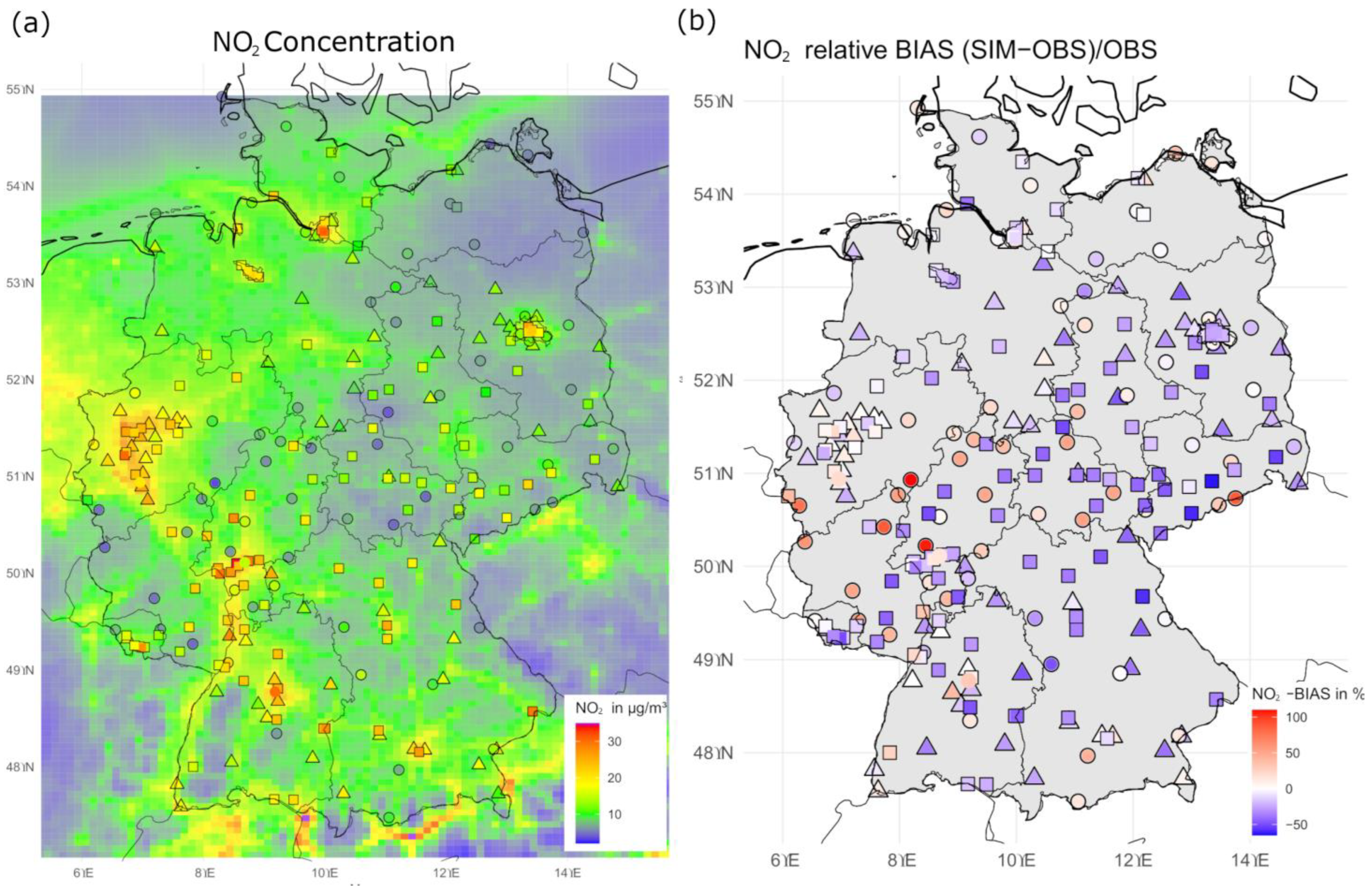
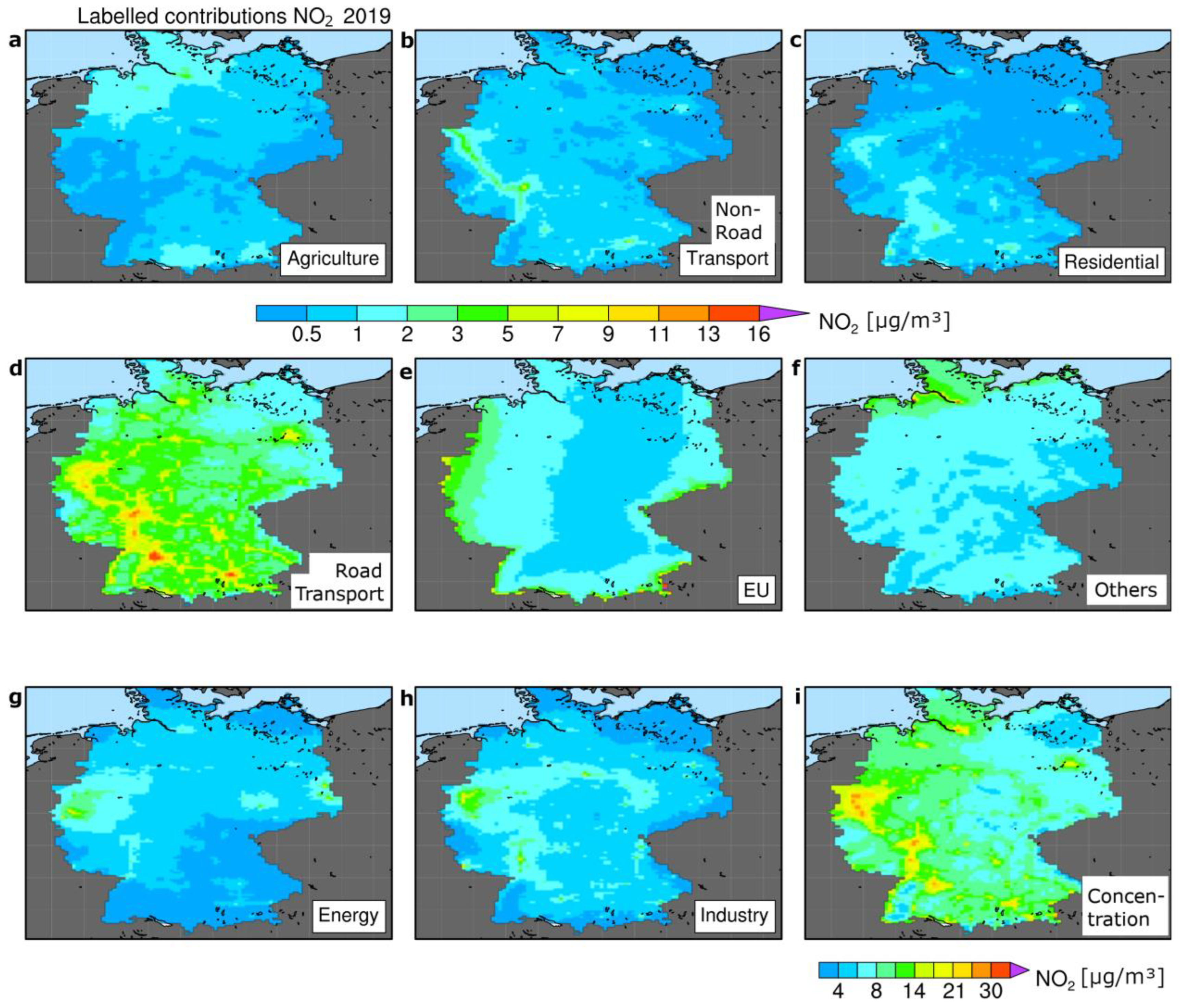
3.1. Spatial and Temporal Distribution

As expected, we modelled the highest NO2 concentrations close to the main emission sources in Germany, e.g., urban agglomerations, traffic routes, shipping lanes, and industrial areas (see Figure 2a). For western and southern Germany, higher NO2 concentrations were modelled than in eastern Germany, except for the state capital of Berlin. The concentrations in the former German Democratic Republic (GDR), namely Brandenburg, Mecklenburg-Western Pomerania, Saxony, Saxony-Anhalt, and Thuringia, are significantly lower than in the other federal states. This difference in the gradient can mainly be explained by a larger population density in western and southern Germany, resulting in larger NOX emissions from source sectors like traffic and residential combustion. The Rhine-Ruhr agglomeration and the urbanised areas along the River Main, Stuttgart, and Munich show the highest modelled background concentrations with annual average values above 20 µg/m3. The relatively large regional background NO2 concentration in the northwest of the country is also influenced by emissions from intensive agricultural activities in the region itself and bordering countries. Finally, the annual mean NO2 distribution shows the patterns of the main transport lines that can be attributed to shipping (inland and sea), railways, and traffic, especially motorways. Figure 2b shows the normalised mean bias (%) between the modelled and observed annual mean concentration of NO2. The largest bias appears at the rural background site DENW065 (a mountain station, 641m AMSL) with an overestimation of 174% of the observed NO2 concentrations, shown in dark red in the south-east of North-Rhine Westphalia, while for most sites an underestimation of observed concentrations, with a negative bias of up to 63% in the urban background (DESN017), is found.
Figure 3 (top) illustrates the modelled NO2 concentrations time series for the urban background of Berlin. The source apportionment information provided in the figure will be discussed below. The modelled time series shows a commonly observed pattern of larger concentrations during winter (DJF) and lower concentrations during summer (JJA) due to the combination of lower boundary layer heights and slightly increased emission strengths during winter as compared to summer. The impact of the synoptic weather situations can be observed on top of this seasonal pattern with periods of higher and lower than average values alternating each other, typically every 4 to 5 days. Largest daily mean values (slightly above 40 µg/m3) were modelled for two periods of stagnating weather conditions during February, which keeps the primary pollutants close to the surface. The observed concentrations show very similar behaviour, albeit with concentration levels larger than modelled in the urban background. In the next section, we discuss the model results in comparison to the available measurement data in Germany in detail.

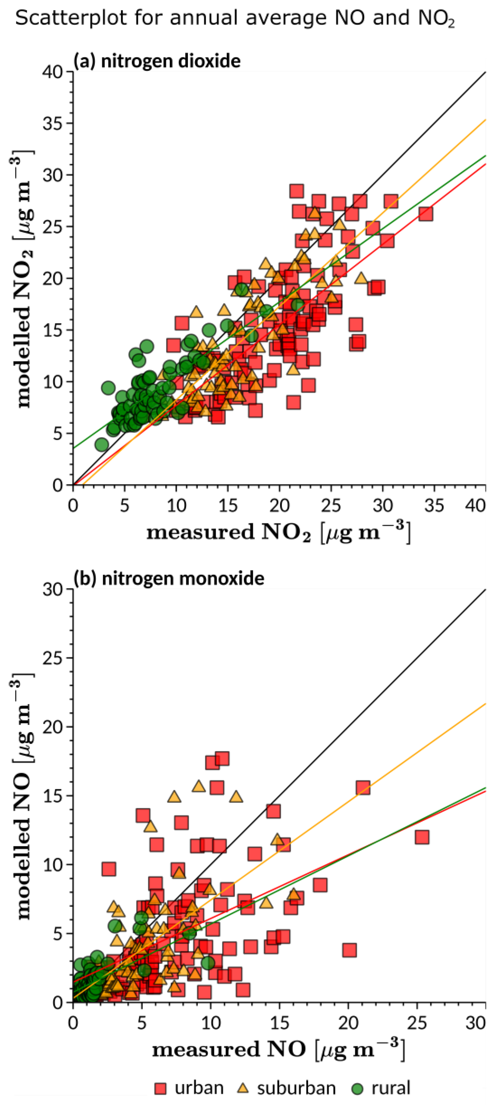
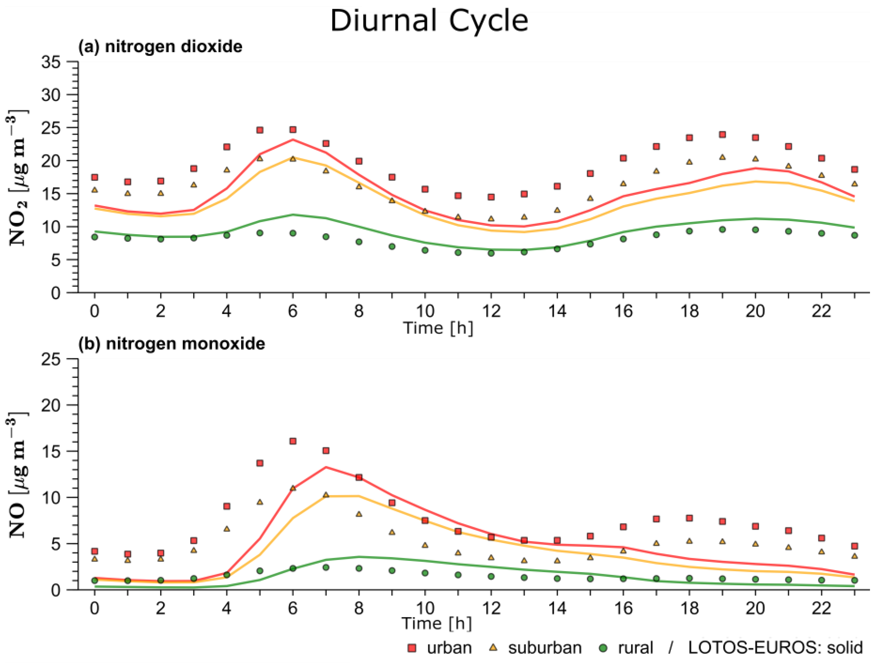
3.2. Comparison Against Observations

The operational model evaluation for NO and NO2 has been performed by calculating statistical metrices (mean bias: MB, root mean squared error: RMSE, index of agreement: IOA and temporal correlation: R) for hourly and daily timeseries, which are summarised in Table 2. The modelled distribution shows very similar patterns with respect to the observations in the regional background (Figure 2). The evaluation shows larger model-measurement agreement in the rural background compared to urban background sites. This is illustrated by larger deviations from the 1:1 line in the scatter diagrams for urban and suburban locations (Figure 4). The modelled hourly concentrations in the rural background show a positive bias of about 1.2 µg/m3 for NO2, while a systematic underestimation of about 4.4 µg/m3 is observed for the urban background stations. No clear bias from the hourly data is evident for NO in the rural area, while in urban regions, the bias is about −2.8 µg/m3 on average. The larger scatter in NO (see Figure 4) is explained by the fact that NO build-up takes place under rather stable conditions after all available ozone has been titrated away. Therefore, modelled NO is also sensitive to the degree in which the emission inventory is representative of local conditions. Hence, such a phenomenon is more difficult to model, and the agreement depends on more factors. This illustrates the ability to correctly model large-scale patterns and the challenge to account for the variability between urban centres. The region of underpredictions in the scatterplot for NO2 corresponds to the stations in cities in the south and east of the country (see Figure 2b). The observed pattern for urban background sites was found for all models in a recent model intercomparison exercise [41].
On average, the model performance is better on a daily basis (R = 0.72) for NO2 than on an hourly basis (R = 0.58), as the daily timeseries are more sensitive to the synoptic variability, which is easier to reproduce than variabilities induced by meteorological and emission dynamics on an hourly time scale. The model reproduces the average diurnal (Figure 5) and weekly cycles of NO and NO2 fairly well. The observed double peak structure for NO2 and the more pronounced morning peak for NO in the diurnal concentration cycle in urban areas are well captured by the model. The NO and NO2 concentration peaks during the morning can be explained by the shallow boundary layer and high NO emissions during rush hour (Figure 5). The afternoon rush hour starts with higher ozone levels and a well-mixed and deep boundary layer for most time of the year and explains the lower peak in NO at around 18:00 UTC. This observed peak in NO around 18:00 UTC is not well captured by the model and may be influenced by an overestimation of ozone levels in the afternoon here, see Thürkow et al. [41]). Moreover, the underestimation of both NO and NO2 in the urban areas hint at an underestimation of urban NOX emissions, as also highlighted by, e.g., Kuik et al. [49]. As an example, Figure 3 provides the comparison for modelled NO2 concentration time series for Berlin and its surroundings. These time series clearly show the good representation of the regional background variability and the clear underestimation of the contrast between urban and rural stations. A recent study on air quality forecasting for Hamburg and other cities also identified an underestimation of innercity NOx emissions [50]. In a follow up, the team simply scaled the urban emissions by the correction factor derived by Kuik et al. [49] to overcome this issue [51]. This underestimation will be discussed below in more detail. Note that for rural background stations far away from source regions, a daytime NO maximum due to photolysis of NO2 is observed and modelled around noon. As we made use of static time profiles using a single diurnal cycle for all days of the week in this modelling exercise, a positive model bias is observed at the weekend. The differences in diurnal cycles between the different weekdays can be introduced in a future study using a dynamic and activity dependent time profiles. In fact, solving the one-hour mismatch in the timing of the peaks in the diurnal cycle has to be sought in the same direction, as the timing depends on the interplay between the emission dynamics and the (onset of) vertical mixing in the morning as well as nighttime ozone levels for NO. For traffic, for example, it would be required to differentiate the temporal variability of emissions from vans, trucks, and commuting light-duty traffic on the different parts of the road network, which is currently not available to us.
Table 2. Overview of the statistical performance indicators of the modelled NO2 and NO timeseries compared to observations. The indicators are mean bias (MB; µg/m3), Root Mean Squared Error (RMSE; µg/m3), Index of Agreement (IOA, see [52]) and the temporal correlation coefficient (R). The values represent the means over all available stations.
(a) NO2MBRMSEIOAR
Hourlyall−2.2810.640.720.58
urban−4.4112.700.710.57
suburban−2.3510.930.730.58
rural1.197.070.720.59
Dailyall−2.297.110.770.72
urban−4.438.710.750.71
suburban−2.376.920.800.73
rural1.184.750.790.72
(b) NO
Hourlyall−1.5713.550.460.33
urban−2.7818.560.490.33
suburban−1.2614.430.470.31
rural0.014.760.390.35
Dailyall−1.498.050.570.50
urban−2.6211.160.620.52
suburban−1.188.420.610.52
rural0.012.650.460.45

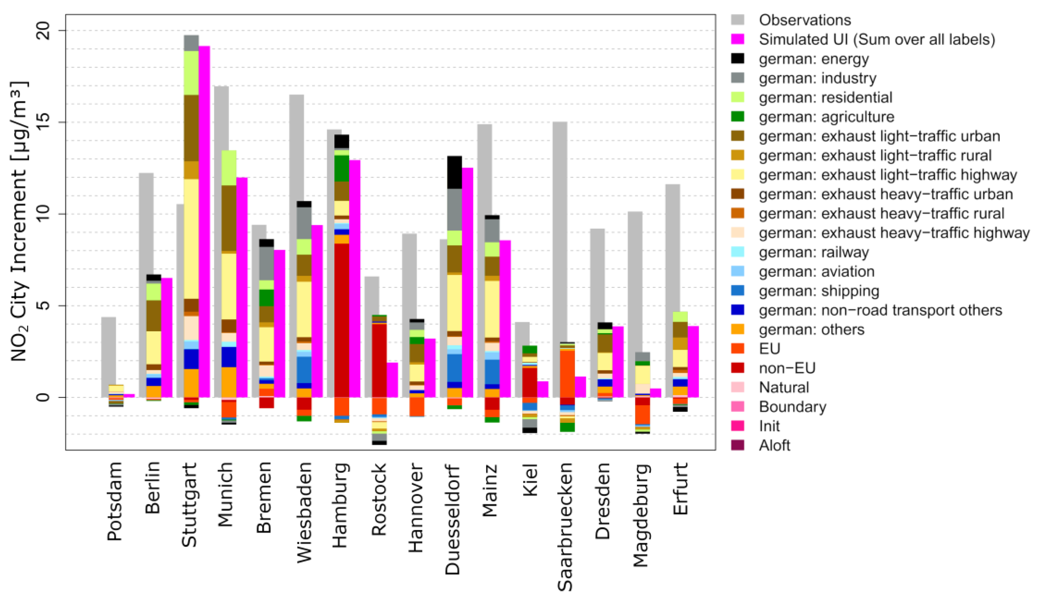
3.3. Source Attribution

Figure 6 shows maps with the modelled contributions of the source sector categories defined and explained in the methodology section. The source attribution for the 16 federal state capitals is detailed in Figure 7. The figure shows the absolute and relative contributions to the urban and rural background on an annual average. Figure 3 shows daily averages for the city of Berlin.
The emissions from road transport contribute most to the annual average concentration of NO2 in the German background. The exceptions are the contributions from abroad near the borders and the contribution of international shipping near the coast. The contribution of road transport in the urban background is on average larger than in the rural background (UB: 41%; RB: 33%) and is in line with the recent literature [53,54]. The largest contributions of road transport were observed for the larger cities in the west and south of Germany, namely Stuttgart (~59%, 14.2 µg/m3), Munich (~55%, 13.2 µg/m3), and Frankfurt/Main (~50%). Note, emissions from light-duty vehicles contribute about 4/5 to road-transport and about 1/5 is attributed to emissions from heavy-duty vehicles. Counterintuitively, we model a larger contribution from highway traffic (~29%) in the urban background than from traffic on the urban roads (~11%). This is partly related to the spatial distribution of cold-start emissions and is further discussed in Section 3.4.
The annual average contribution of inland shipping emissions is about 3% and was mainly observed along the larger rivers (e.g., the Rhine). At the German coasts (North and Baltic Sea), emissions from international shipping (labelled as non-EU) show large contributions, with largest contributions in the federal state capitals Hamburg (~31%, 8.6 µg/m3), Rostock (~39%, 4.5 µg/m3), and Kiel (~22%, 2.3 µg/m3). These results are in line with those of Tokaya et al. [55] ranging from 6.5% to 62% for major European harbour cities on the North Sea coast. For the city of Hamburg, their results were about 41% (11.5 µg/m3) because they used a finer-resolved model and selected certain grid points representing the city centre and the harbour, while our selection was limited to the observation site. Aviation and rail traffic explain the rest of the non-road emissions and contribute about 2% to the annual average NO2 concentration in Germany. About 3% to 11% was attributed to emissions from residential combustion. The contributions from residential combustion are more evenly distributed with a gradient from the densely populated south (Rhine-Ruhr conurbation, Stuttgart, and Frankfurt/Main) to the sparsely populated north-east of Germany. Emissions from power plants in the lignite region of Lusatia near the Polish border and in the Rhine-Ruhr metropolitan region show an increased contribution of energy production to the NO2 concentration of up to 14% compared to only 3% in the regional background. We observed the typical characteristics with increased contributions in winter of residential combustion in the urban background (winter: ~9%; summer: ~3%) and energy production (winter: ~7%; summer: ~6%), which can be explained by the heating season during the cold period [48]. The emissions from industry show large regional differences in Germany, with peak values in the interior (~11%) and western parts (~13%) of the country. The lowest contribution of industry was observed for the north-east of Germany. Agriculture shows largest contribution in the northern parts of Germany (Schleswig Holstein: ~9% and Lower Saxony: ~14%) and largely varies in time with the maximum contribution during the spring period (MAM, up to ~13%).
Obviously, modelled transboundary contributions are largest at the German domestic borders (~30%). Largest values for European contributions were observed in south-east Germany of about 60%, close to the borders of Austria and the Czech Republic. The federal state capital with the largest transboundary contribution (label EU) to the urban background is Saarbrucken with about 30% (~4 µg/m3). A lower contribution was observed along the north-eastern German borders (~10%). The contribution from other European countries is about 5% in summer and can make up to 14% in winter in the urban background of the federal state capitals. All other source contributions show maximal annual average contributions of 6.1% in the rural background (natural), while the remaining sectors contribute below 3.2%.
Figure 8 shows the modelled and observed difference or city increment between the urban background and rural background NO2 concentration for the 16 federal state capitals. The difference is calculated for each source sector category. Note that negative values may occur for some source categories, indicating a larger contribution in the rural background. The largest average differences were modelled for some of the larger federal state capitals, such as Munich (16.9 µg/m3), Wiesbaden (16.5 µg/m3), Hamburg (14.7 µg/m3), and Mainz (14.8 µg/m3). The lowest differences are modelled for Potsdam (0.2 µg/m3), Magdeburg (0.5 µg/m3), Kiel (0.8 µg/m3), and Saarbrücken (1.2 µg/m3). Apart from Stuttgart and Düsseldorf, the annual mean city increment of NO2 derived from observations is underestimated by the model by about 52% (~5.3 µg/m3). Only for Stuttgart is the modelled difference much larger than observed. The locations of the rural background sites used for the calculation for Stuttgart are quite close to the city border. This shows that the horizontal grid resolution and the specific location of a station may not allow for correctly depicting such small-scale differences and must always be considered carefully.
The city increments for traffic are always positive with the largest contributions (~66%, Stuttgart) to the total increment. Highway contributions (~22%, all) explain about a third of this traffic-induced increment. Emissions from international shipping show large positive contributions in Hamburg (~53%), Rostock (~56%), and Kiel (~34%), while inland shipping emissions mainly contribute to the city increment in Wiesbaden (~12%), Düsseldorf (~11%, ~1.8 µg/m3), and Mainz (~12%). For some sectors, the modelled rural concentrations are larger than those in the cities. This is, for example, the case for Saarbrücken and Wiesbaden, whereas this is not the case for Bremen and Hamburg (see Figure 7 c,d). Also, for energy and industry both positive and negative increments are found. For example, for Duesseldorf the attributed concentration in the urban background is larger than in the surrounding areas, explaining about a third of the city’s increment (29%). The sign of the differences between the urban and regional background stations depends on the configurations of the measurement network and the location of the sources. This is clearly illustrated by the often-negative transboundary increments, as the location of the rural background stations tend to be closer to the border than the federal state capitals. Ideally, the model should be able to represent the observed differences and correctly explain the respective source contributions, as the model includes the source information and the process descriptions to model the NO2 behaviour in the different regions. This is, however, not the case, with often a significant underestimation of the observed difference between urban and rural background concentration levels. To address how far shortcomings in the representation of urban emissions drive the underestimation of the city increments, it is advisable to take the most isolated city with a low emission density around it as the case study, i.e., Berlin.

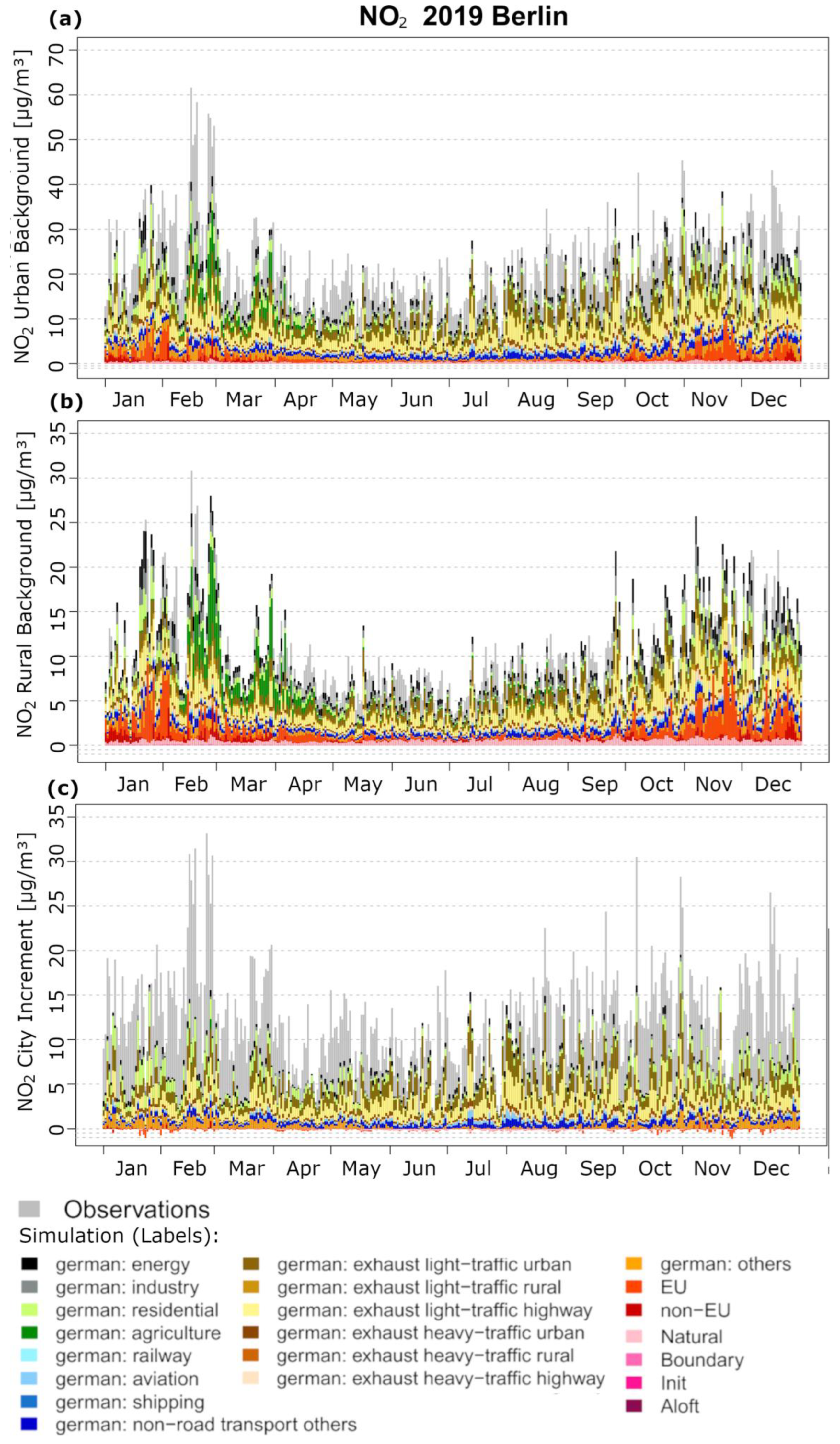
3.4. Case Study Berlin

The observed concentration of NO2 shows a strong variation, changing with the daily mean temperature in Berlin (Figure 9). The mean concentration on days with freezing conditions is almost a factor of 2 larger than on days with mean temperatures around 15 °C. The concentrations show a declining trend with increasing temperature, until concentrations start to rise again in hot summer conditions. The modelled mean urban background levels show an underestimation of cold days (~12% for 0–5 °C) and of warm days (~42% for 30–35 °C). In the rural background, a similar temperature dependency is found as in the urban areas, with an overestimation of observed concentrations for cold days (~8%) and an underestimation for warm days (~26%). The city increment for Berlin derived from observations shows a minimum on days with temperatures of around 25 degrees and tends to be larger for colder and warmer conditions. Although the model captures the overall temperature dependency for NO2 with temperature, the modelled city increment, in contrast, is almost constant and only increases for freezing conditions. Hence, the relation between the urban NO2 concentrations and temperature is stronger in the city than in its surroundings, which is not reflected by the model results.
We attribute the general increase with decreasing temperature found in the greater Berlin area to the influence of the synoptic situations with less ventilation due to lower wind speeds and lower mixing layer heights during winter conditions [24,56,57,58], in combination with enhanced emissions during cold conditions. Figure 9 also shows that the contribution of residential combustion is by a factor of 6 larger on days with freezing conditions than during summer conditions as a result of the heating degree days approach used in LOTOS-EUROS to replace static time profiles and to model the temporal emission variability of this source sector [48]. For residential combustion, we also observed the largest NO2-sensitivity to temperature in the urban background with a contribution ranging from about 3% (warm conditions, in JJA) to about 18% (cold conditions, in DJF). Road transport shows a lower contribution for cold days (~39% for 0–5 °C) than for warm days (~65% for 30–35 °C). Its absolute contribution to the city increment remains rather constant with temperature.
The representation of the traffic emissions may explain a part of the mismatch for the city increment and the underestimation of urban NO2 levels in general. Firstly, in many emissions inventories, the impact of cold starts are included in the calculation of the effective emission factors for the car type per road type. The national emissions are then calculated based on the kilometres driven per road type and car type. Next, the emission totals for traffic are distributed across the road network (by different teams) based on kilometres driven. This procedure causes the contribution of the cold starts to the emission totals to be spread across the whole network. In reality, the cold starts largely take place in residential areas (in the morning) and in working areas (in the afternoon), and thus in urban areas; hence, the traffic emissions in the cities may be underestimated in general. This effect is becoming more important as the relative share of the cold start to the emissions of a single trip is increasing for modern cars [59,60]. Secondly, recent studies also show that traffic emissions during hot engine conditions also depend on temperature [53,61]. Wærsted et al. [59] show a two times larger emission factor for diesel engine cars during cold conditions (0 to 5 °C) than at around 20 degrees in Norway. These findings need to be confirmed for German conditions, but hint at a requirement to also detail the variability of hot engine traffic emissions in future modelling applications.
Other sources may also show meteorological dependencies that are not accommodated by the currently used time profiles. Similar to traffic, it may be necessary to further detail the NOX-temperature sensitivity for other motorised sources, e.g., mobile machinery, diesel trains. The mismatch of the city increment for warm days may be partly attributed to an increase in human activity, i.e., energy use and emissions from air conditioning, traffic, and tourist activities. These effects make the urban area more energy inefficient [62] but are not accounted for yet. In addition, the representation of the urban photochemical regime during such hot conditions, including NOX cycling and NOX lifetime, as well as the role of reservoir species like PAN, deserves further attention.

4. Conclusions

In this study, we have successfully applied the LOTOS-EUROS model to address the source attribution of nitrogen dioxide for regional and urban background conditions in Germany. The study is a follow-up of the evaluation of the labelling methodology for NO2 described by Thürkow et al. [37] by detailing a much larger set of source sectors and focusing on the source apportionment results and the evaluation for federal state capitals, including Berlin. The model evaluation showed a systematic underestimation of NO2 levels in urban areas, similar to previous studies, while for regional background areas, a slight overestimation was observed. In the corresponding source apportionment, road transport was identified as the largest contributor, particularly in urban background settings (on average 41%, up to 59% in major cities), with larger shares from light-duty vehicles than from heavy-duty vehicles. Modelled contributions from traffic on highways exceeded those from urban roads, but they may be too large, as they include an impact from cold starts emissions. This study also highlights contributions from shipping, agriculture, energy, and industry, which vary significantly from region to region. Transboundary contributions also play a role, particularly near the German border. The underestimation of NO2 in urban areas motivated a more detailed analysis of Berlin. The observed city increment for Berlin shows a large sensitivity to ambient temperature, which is not reproduced by the model. The current spatial allocation of the traffic emissions based on kilometres driven may spread the temperature dependent contribution of cold-start emissions across the whole network, although these may largely occur in cities. These results indicate that the way the traffic emissions are described, and especially the temperature influence, needs to be updated. We recommend separately estimating and spatially distributing the emissions from cold starts in the German inventory. In addition, we recommend detailing the time profiles for different parts of the fleet, and exploring the impact of temperature on hot traffic emissions further. We speculate that the current assessments of air quality improvement, which overlook these temperature-related impacts on emissions, may be overly optimistic about meeting the new EU air quality standards in urban areas.

Author Contributions

Conceptualization, J.P., M.T. and M.S.; methodology, J.P., M.T. and M.S.; validation, M.T. and J.P.; formal analysis, J.P. and M.T.; writing—original draft preparation, J.P. and M.T.; writing—review and editing, S.B. and M.S.; visualisation, J.P.; supervision, S.B. and M.S.; funding acquisition, M.S. All authors have read and agreed to the published version of the manuscript.

Funding

This research was funded by Horizon Europe framework programme projects FONDA, grant number 101079134, and MI-TRAP, grant number 101138449.

Institutional Review Board Statement

Not applicable.

Informed Consent Statement

Not applicable.

Data Availability Statement

All modelling results are available upon request.

Acknowledgments

The authors would like to thank the HPC Service of ZEDAT, Freie Universität Berlin, for computing time [63].

Conflicts of Interest

The authors declare no conflicts of interest.

References

  1. Newby, D.E.; Mannucci, P.M.; Tell, G.S.; Baccarelli, A.A.; Brook, R.D.; Donaldson, K.; Forastiere, F.; Franchini, M.; Franco, O.H.; Graham, I.; et al. Expert Position Paper on Air Pollution and Cardiovascular Disease. Eur. Heart J. 2015, 36, 83–93. [Google Scholar] [CrossRef] [PubMed]
  2. Faustini, A.; Rapp, R.; Forastiere, F. Nitrogen Dioxide and Mortality: Review and Meta-Analysis of Long-Term Studies. Eur. Respir. J. 2014, 44, 744–753. [Google Scholar] [CrossRef]
  3. Huang, S.; Li, H.; Wang, M.; Qian, Y.; Steenland, K.; Caudle, W.M.; Liu, Y.; Sarnat, J.; Papatheodorou, S.; Shi, L. Long-Term Exposure to Nitrogen Dioxide and Mortality: A Systematic Review and Meta-Analysis. Sci. Total Environ. 2021, 776, 145968. [Google Scholar] [CrossRef] [PubMed]
  4. Raaschou-Nielsen, O.; Andersen, Z.J.; Jensen, S.S.; Ketzel, M.; Sørensen, M.; Hansen, J.; Loft, S.; Tjønneland, A.; Overvad, K. Traffic Air Pollution and Mortality from Cardiovascular Disease and All Causes: A Danish Cohort Study. Environ. Health 2012, 11, 60. [Google Scholar] [CrossRef]
  5. European Environment Agency. Air Quality in Europe 2022; European Environment Agency: Copenhagen, Denmark, 2023. [Google Scholar]
  6. Huangfu, P.; Atkinson, R. Long-Term Exposure to NO2 and O3 and All-Cause and Respiratory Mortality: A Systematic Review and Meta-Analysis. Environ. Int. 2020, 144, 105998. [Google Scholar] [CrossRef]
  7. van Pinxteren, D.; Engelhardt, V.; Mothes, F.; Poulain, L.; Fomba, K.W.; Spindler, G.; Cuesta-Mosquera, A.; Tuch, T.; Müller, T.; Wiedensohler, A.; et al. Residential Wood Combustion in Germany: A Twin-Site Study of Local Village Contributions to Particulate Pollutants and Their Potential Health Effects. ACS Environ. Au 2024, 4, 12–30. [Google Scholar] [CrossRef]
  8. WHO Regional Office for Europe. Economic Cost of the Health Impact of Air Pollution in Europe Clean Air, Health and Wealth; WHO Regional Office for Europe: Copenhagen, Denmark, 2015. [Google Scholar]
  9. COMEAP. Statement on the Evidence for the Effects of Nitrogen Dioxide on Health. In Committe on the Medical Effects or Air Pollutants; UK Government: London, UK, 2015. [Google Scholar]
  10. Fischer, P.H.; Marra, M.; Ameling, C.B.; Hoek, G.; Beelen, R.; De Hoogh, K.; Breugelmans, O.; Kruize, H.; Janssen, N.A.H.; Houthuijs, D. Air Pollution and Mortality in Seven Million Adults: The Dutch Environmental Longitudinal Study (DUELS). Environ. Health Perspect. 2015, 123, 697–704. [Google Scholar] [CrossRef] [PubMed]
  11. Anenberg, S.C.; Mohegh, A.; Goldberg, D.L.; Kerr, G.H.; Brauer ScD, M.; Burkart, K.; Wozniak, S.B.; Hystad, P.; Larkin, A.; Anenberg, S.C.; et al. Long-Term Trends in Urban NO2 Concentrations and Associated Paediatric Asthma Incidence: Estimates from Global Datasets. Lancet Planet. Health 2022, 6, e49–e58. [Google Scholar] [CrossRef]
  12. Erickson, L.E.; Newmark, G.L.; Higgins, M.J.; Wang, Z. Nitrogen Oxides and Ozone in Urban Air: A Review of 50 plus Years of Progress. Environ. Prog. Sustain. Energy 2020, 39, e13484. [Google Scholar] [CrossRef]
  13. European Environment Agency. Air Quality in Europe: 2020 Report; Publications Office of the European Union: Copenhagen, Denmark, 2020; ISBN 9789294802927. [Google Scholar]
  14. Umweltbundesamt Luftqualität. 2020 Vorläufige Auswertung; Umweltbundesamt Luftqualität: Dessau-Roßlau, Germany, 2021. [Google Scholar]
  15. European Commission. I Directive 2008/50/EC of the European Parliament and of the Council of 21 May 2008 on Ambient Air Quality and Cleaner Air for Europe; European Commission: Brussels, Belgium, 2008. [Google Scholar]
  16. Umweltbundesamt Luftqualität. 2023 (Vorläufige Auswertung); Umweltbundesamt Luftqualität: Dessau-Roßlau, Germany, 2024. [Google Scholar]
  17. World Health Organization. WHO Global Air Quality Guidelines. Particulate Matter (PM2.5 and PM10), Ozone, Nitrogen Dioxide, Sulfur Dioxide and Carbon Monoxide; WHO: Geneva, Switzerland, 2021. [Google Scholar]
  18. European Commission. Proposal for a Directive of the European Parliament and of the Council on Ambient Air Quality and Cleaner Air for Europe (Recast); European Commission: Brussels, Belgium, 2022. [Google Scholar]
  19. Nuvolone, D.; Petri, D.; Voller, F. The Effects of Ozone on Human Health. Environ. Sci. Pollut. Res. 2018, 25, 8074–8088. [Google Scholar] [CrossRef]
  20. Bromberg, P.A. Mechanisms of the Acute Effects of Inhaled Ozone in Humans. Biochim. Biophys. Acta (BBA)-Gen. Subj. 2016, 1860, 2771–2781. [Google Scholar] [CrossRef] [PubMed]
  21. Holm, S.M.; Balmes, J.R. Systematic Review of Ozone Effects on Human Lung Function, 2013 Through 2020. Chest 2022, 161, 190–201. [Google Scholar] [CrossRef]
  22. Sandermann, H. Ozone and Plant Health. Annu. Rev. Phytopathol. 1996, 34, 347–366. [Google Scholar] [CrossRef]
  23. Agathokleous, E.; Feng, Z.; Oksanen, E.; Sicard, P.; Wang, Q.; Saitanis, C.J.; Araminiene, V.; Blande, J.D.; Hayes, F.; Calatayud, V.; et al. Ozone Affects Plant, Insect, and Soil Microbial Communities: A Threat to Terrestrial Ecosystems and Biodiversity. Sci. Adv. 2020, 6, eabc1176. [Google Scholar] [CrossRef] [PubMed]
  24. van Pinxteren, D.; Mothes, F.; Spindler, G.; Fomba, K.W.; Herrmann, H. Trans-Boundary PM10: Quantifying Impact and Sources during Winter 2016/17 in Eastern Germany. Atmos. Environ. 2019, 200, 119–130. [Google Scholar] [CrossRef]
  25. Garcia, A.; Santa-Helena, E.; De Falco, A.; de Paula Ribeiro, J.; Gioda, A.; Gioda, C.R. Toxicological Effects of Fine Particulate Matter (PM2.5): Health Risks and Associated Systemic Injuries—Systematic Review. Water Air Soil Pollut. 2023, 234, 346. [Google Scholar] [CrossRef] [PubMed]
  26. Fowler, D.; Coyle, M.; Skiba, U.; Sutton, M.A.; Cape, J.N.; Reis, S.; Sheppard, L.J.; Jenkins, A.; Grizzetti, B.; Galloway, J.N.; et al. The Global Nitrogen Cycle in the Twenty-First Century. Philos. Trans. R. Soc. B Biol. Sci. 2013, 368, 20130164. [Google Scholar] [CrossRef]
  27. Jonson, J.E.; Fagerli, H.; Scheuschner, T.; Tsyro, S. Modelling Changes in Secondary Inorganic Aerosol Formation and Nitrogen Deposition in Europe from 2005 to 2030. Atmos. Chem. Phys. 2022, 22, 1311–1331. [Google Scholar] [CrossRef]
  28. Butler, T.; Lupascu, A.; Coates, J.; Zhu, S. TOAST 1.0: Tropospheric Ozone Attribution of Sources with Tagging for CESM 1.2.2. Geosci. Model Dev. 2018, 11, 2825–2840. [Google Scholar] [CrossRef]
  29. Bartík, L.; Huszár, P.; Karlický, J.; Vlček, O.; Eben, K. Modeling the Drivers of Fine PM Pollution over Central Europe: Impacts and Contributions of Emissions from Different Sources. Atmos. Chem. Phys. 2024, 24, 4347–4387. [Google Scholar] [CrossRef]
  30. Pültz, J.; Banzhaf, S.; Thürkow, M.; Kranenburg, R.; Schaap, M. Source Attribution of Particulate Matter in Berlin. Atmos. Environ. 2023, 292, 119416. [Google Scholar] [CrossRef]
  31. Carruthers, D.J.; Edmunds, H.A.; Lester, A.E.; McHugh, C.A.; Singles, R.J. Use and Validation of ADMS-Urban in Contrasting Urban and Industrial Locations. Int. J. Environ. Pollut. 2000, 14, 364–374. [Google Scholar] [CrossRef]
  32. Schiavon, M.; Redivo, M.; Antonacci, G.; Rada, E.C.; Ragazzi, M.; Zardi, D.; Giovannini, L. Assessing the Air Quality Impact of Nitrogen Oxides and Benzene from Road Traffic and Domestic Heating and the Associated Cancer Risk in an Urban Area of Verona (Italy). Atmos. Environ. 2015, 120, 234–243. [Google Scholar] [CrossRef]
  33. Tilloy, A.; Mallet, V.; Poulet, D.; Pesin, C.; Brocheton, F. BLUE-Based NO2 Data Assimilation at Urban Scale. J. Geophys. Res. Atmos. 2013, 118, 2031–2040. [Google Scholar] [CrossRef]
  34. Wagstrom, K.M.; Pandis, S.N.; Yarwood, G.; Wilson, G.M.; Morris, R.E. Development and Application of a Computationally Efficient Particulate Matter Apportionment Algorithm in a Three-Dimensional Chemical Transport Model. Atmos. Environ. 2008, 42, 5650–5659. [Google Scholar] [CrossRef]
  35. Belis, C.A.; Pirovano, G.; Villani, M.G.; Calori, G.; Pepe, N.; Putaud, J.P. Comparison of Source Apportionment Approaches and Analysis of Non-Linearity in a Real Case Model Application. Geosci. Model Dev. 2021, 14, 4731–4750. [Google Scholar] [CrossRef]
  36. Clappier, A.; Belis, C.A.; Pernigotti, D.; Thunis, P. Source Apportionment and Sensitivity Analysis: Two Methodologies with Two Different Purposes. Geosci. Model Dev. 2017, 10, 4245–4256. [Google Scholar] [CrossRef]
  37. Thürkow, M.; Banzhaf, S.; Butler, T.; Pültz, J.; Schaap, M. Source Attribution of Nitrogen Oxides across Germany: Comparing the Labelling Approach and Brute Force Technique with LOTOS-EUROS. Atmos. Environ. 2023, 292, 119412. [Google Scholar] [CrossRef]
  38. Marécal, V.; Peuch, V.H.; Andersson, C.; Andersson, S.; Arteta, J.; Beekmann, M.; Benedictow, A.; Bergström, R.; Bessagnet, B.; Cansado, A.; et al. A Regional Air Quality Forecasting System over Europe: The MACC-II Daily Ensemble Production. Geosci. Model Dev. 2015, 8, 2777–2813. [Google Scholar] [CrossRef]
  39. Pommier, M.; Fagerli, H.; Schulz, M.; Valdebenito, A.; Kranenburg, R.; Schaap, M. Prediction of Source Contributions to Urban Background PM10 Concentrations in European Cities: A Case Study for an Episode in December 2016 Using EMEP/MSC-W Rv4.15 and LOTOS-EUROS v2.0—Part 1: The Country Contributions. Geosci. Model Dev. 2020, 13, 1787–1807. [Google Scholar] [CrossRef]
  40. Bessagnet, B.; Pirovano, G.; Mircea, M.; Cuvelier, C.; Aulinger, A.; Calori, G.; Ciarelli, G.; Manders, A.; Stern, R.; Tsyro, S.; et al. Presentation of the EURODELTA III Intercomparison Exercise-Evaluation of the Chemistry Transport Models’ Performance on Criteria Pollutants and Joint Analysis with Meteorology. Atmos. Chem. Phys. 2016, 16, 12667–12701. [Google Scholar] [CrossRef]
  41. Thürkow, M.; Schaap, M.; Kranenburg, R.; Pfäfflin, F.; Neunhäuserer, L.; Wolke, R.; Heinold, B.; Stoll, J.; Lupaşcu, A.; Nordmann, S.; et al. Dynamic Evaluation of Modeled Ozone Concentrations in Germany with Four Chemistry Transport Models. Sci. Total Environ. 2024, 906, 167665. [Google Scholar] [CrossRef] [PubMed]
  42. Manders, A.M.M.; Builtjes, P.J.H.; Curier, L.; Denier van der Gon, H.A.; Hendriks, C.; Jonkers, S.; Kranenburg, R.; Kuenen, J.J.P.; Segers, A.J.; Timmermans, R.M.A.; et al. Curriculum Vitae of the LOTOS-EUROS (v2.0) Chemistry Transport Model. Geosci. Model Dev. 2017, 10, 4145–4173. [Google Scholar] [CrossRef]
  43. Reinert, D.; Prill, F.; Frank, H.; Zängl, G. ICON Database Reference Manual; Deutscher Wetterdienst: Offenbach, Germany, 2015. [Google Scholar]
  44. Inness, A.; Ades, M.; Agustí-Panareda, A.; Barr, J.; Benedictow, A.; Blechschmidt, A.M.; Jose Dominguez, J.; Engelen, R.; Eskes, H.; Flemming, J.; et al. The CAMS Reanalysis of Atmospheric Composition. Atmos. Chem. Phys. 2019, 19, 3515–3556. [Google Scholar] [CrossRef]
  45. Kuenen, J.; Dellaert, S.; Visschedijk, A.; Jalkanen, J.P.; Super, I.; Denier Van Der Gon, H. CAMS-REG-v4: A State-of-the-Art High-Resolution European Emission Inventory for Air Quality Modelling. Earth Syst. Sci. Data 2022, 14, 491–515. [Google Scholar] [CrossRef]
  46. Schneider, C.; Pelzer, M.; Toenges-Schuller, N.; Nacken, M.; Niederau, A. ArcGIS Basierte Lösung Zur Detaillierten, Deutsch-Landweiten Verteilung (Gridding) Nationaler Emissionsjahreswerte Auf Basis Des Inventars Zur Emissionsbericht-Erstattung Langfassung. Dessau. Roßlau Retrieved 2016, 27, 2019. [Google Scholar]
  47. Kaiser, J.W.; Heil, A.; Andreae, M.O.; Benedetti, A.; Chubarova, N.; Jones, L.; Morcrette, J.J.; Razinger, M.; Schultz, M.G.; Suttie, M.; et al. Biomass Burning Emissions Estimated with a Global Fire Assimilation System Based on Observed Fire Radiative Power. Biogeosciences 2012, 9, 527–554. [Google Scholar] [CrossRef]
  48. Denier Van Der Gon, H.A.C.; Bergström, R.; Fountoukis, C.; Johansson, C.; Pandis, S.N.; Simpson, D.; Visschedijk, A.J.H. Particulate Emissions from Residential Wood Combustion in Europe—Revised Estimates and an Evaluation. Atmos. Chem. Phys. 2015, 15, 6503–6519. [Google Scholar] [CrossRef]
  49. Kuik, F.; Kerschbaumer, A.; Lauer, A.; Lupascu, A.; Von Schneidemesser, E.; Butler, T.M. Top-down Quantification of NOx Emissions from Traffic in an Urban Area Using a High-Resolution Regional Atmospheric Chemistry Model. Atmos. Chem. Phys. 2018, 18, 8203–8225. [Google Scholar] [CrossRef]
  50. Karl, M.; Acksen, S.; Chaudhary, R.; Ramacher, M.O.P. Forecasting System for Urban Air Quality with Automatic Correction and Web Service for Public Dissemination. Int. J. Digit. Earth 2024, 17, 1–22. [Google Scholar] [CrossRef]
  51. Ramacher, M.O.P.; Badeke, R.; Fink, L.; Quante, M.; Karl, M.; Oppo, S.; Lenartz, F.; Dury, M.; Matthias, V. Assessing the Effects of Significant Activity Changes on Urban-Scale Air Quality across Three European Cities. Atmos. Environ. X 2024, 22, 100264. [Google Scholar] [CrossRef]
  52. Janssen, S.; Thunis, P. FAIRMODE Guidance Document on Modelling Quality Objectives and Benchmarking (version 3.3); EUR 31068 EN; Publications Office of the European Union: Luxembourg, 2022; ISBN 978-92-76-52425-0. [Google Scholar]
  53. Grange, S.K.; Farren, N.J.; Vaughan, A.R.; Rose, R.A.; Carslaw, D.C. Strong Temperature Dependence for Light-Duty Diesel Vehicle NOx Emissions. Environ. Sci. Technol. 2019, 53, 6587–6596. [Google Scholar] [CrossRef] [PubMed]
  54. Kuik, F.; Lauer, A.; Churkina, G.; Denier Van Der Gon, H.A.C.; Fenner, D.; Mar, K.A.; Butler, T.M. Air Quality Modelling in the Berlin-Brandenburg Region Using WRF-Chem v3.7.1: Sensitivity to Resolution of Model Grid and Input Data. Geosci. Model Dev. 2016, 9, 4339–4363. [Google Scholar] [CrossRef]
  55. Tokaya, J.P.; Kranenburg, R.; Timmermans, R.M.A.; Coenen, P.W.H.G.; Kelly, B.; Hullegie, J.S.; Megaritis, T.; Valastro, G. The Impact of Shipping on the Air Quality in European Port Cities with a Detailed Analysis for Rotterdam. Atmos. Environ. X 2024, 23, 100278. [Google Scholar] [CrossRef]
  56. Harkey, M.; Holloway, T.; Oberman, J.; Scotty, E. An Evaluation of CMAQ NO2 using Observed Chemistry-Meteorology Correlations. J. Geophys. Res. 2015, 120, 11775–11797. [Google Scholar] [CrossRef]
  57. Baklanov, A.; Schlünzen, K.; Suppan, P.; Baldasano, J.; Brunner, D.; Aksoyoglu, S.; Carmichael, G.; Douros, J.; Flemming, J.; Forkel, R.; et al. Online Coupled Regional Meteorology Chemistry Models in Europe: Current Status and Prospects. Atmos. Chem. Phys. 2014, 14, 317–398. [Google Scholar] [CrossRef]
  58. Thürkow, M.; Kirchner, I.; Kranenburg, R.; Timmermans, R.M.A.; Schaap, M. A Multi-Meteorological Comparison for Episodes of PM10 Concentrations in the Berlin Agglomeration Area in Germany with the LOTOS-EUROS CTM. Atmos. Environ. 2021, 244, 117946. [Google Scholar] [CrossRef]
  59. Wærsted, E.G.; Sundvor, I.; Denby, B.R.; Mu, Q. Quantification of Temperature Dependence of NOx Emissions from Road Traffic in Norway Using Air Quality Modelling and Monitoring Data. Atmos. Environ. X 2022, 13, 100160. [Google Scholar] [CrossRef]
  60. Jiang, Y.; Song, G.; Wu, Y.; Lu, H.; Zhai, Z.; Yu, L. Impacts of Cold Starts and Hybrid Electric Vehicles on On-Road Vehicle Emissions. Transp. Res. D Transp. Environ. 2024, 126, 104011. [Google Scholar] [CrossRef]
  61. Hall, D.L.; Anderson, D.C.; Martin, C.R.; Ren, X.; Salawitch, R.J.; He, H.; Canty, T.P.; Hains, J.C.; Dickerson, R.R. Using Near-Road Observations of CO, NOy, and CO2 to Investigate Emissions from Vehicles: Evidence for an Impact of Ambient Temperature and Specific Humidity. Atmos. Environ. 2020, 232, 117558. [Google Scholar] [CrossRef]
  62. Roxon, J.; Ulm, F.J.; Pellenq, R.J.M. Urban Heat Island Impact on State Residential Energy Cost and CO2 Emissions in the United States. Urban Clim. 2020, 31, 100546. [Google Scholar] [CrossRef]
  63. Loris Bennett, B.M.B.P. Curta: A General-Purpose High-Performance Computer at ZEDAT; Freie Universität: Berlin, Germany, 2020. [Google Scholar] [CrossRef]
Figure 1. Overview of the inner model domain and measurement sites. Red squares indicate urban background sites. Sites in the suburban and rural background are coded with orange triangles and green circles, respectively. The blue dashed (for rural background) and solid yellow (for urban background) circles show the area covering the measurement sites that were selected for each of the 16 federal state capitals.
Atmosphere 16 00312 g001
Figure 2. (a) Modelled and observed annual mean concentration of NO2 (µg/m3) and (b) the normalised mean bias (%) across Germany. The classification of the measurement sites is in accordance with Figure 1.
Atmosphere 16 00312 g002
Figure 3. Daily time series of NO2 concentration for the urban (a) and rural (b) background and the city increment (c) for Berlin calculated from stations as listed in Table 1. Observed (grey) and modelled values (labels, coloured) are included.
Atmosphere 16 00312 g003
Figure 4. Scatterplots of the annual average NO2 and NO concentrations for urban, suburban, and rural background stations/corresponding grid points. The regression line is plotted for each station class.
Atmosphere 16 00312 g004
Figure 5. Diurnal cycle of observed (symbols) and modelled (solid lines) NO2 (top, (a)) and NO (bottom, (b)) concentrations for urban (red), suburban (orange), and rural (green) sites.
Atmosphere 16 00312 g005
Figure 6. Annual average concentration of NO2 (bottom right, (i)) and the absolute contribution (ah) of the main source categories. Note that the total modelled concentration has a different scale than the other panels.
Atmosphere 16 00312 g006
Figure 7. NO2 Source sector contributions ((a,b)-top: normalised and (c,d)-bottom: absolute) of the 16 federal state capitals in the urban (left) and rural (right) background. The observations are colour-coded in grey.
Atmosphere 16 00312 g007
Figure 8. Observed (grey) and modelled (magenta) city increment. The source sector contributions are colour-coded as defined in the legend.
Atmosphere 16 00312 g008
Figure 9. Observed (grey) and modelled (magenta) daily average NO2-sensitivity to temperature in the urban (a) and the rural (b) backgrounds for Berlin. The NO2-sensitivity to temperature of the city increment is shown in the bottom panel (c). The source sector contributions are colour-coded, as defined in the legend. The temperature interval is 5 °C. At least 10 days were used to calculate the mean to each temperature interval. The data density (number of observations) on the right vertical axis is shown as a solid line (grey line).
Atmosphere 16 00312 g009
Table 1. Information of the 16 federal state capitals with their population, area, city centre, and radius for selection of sites by UBA code. Note that Rostock was chosen as the representative city for Mecklenburg–Western Pomerania, as the state capital Schwerin is missing an observation site.
State CapitalSelected Sites
Name
(State)
Inhabitants (2022)
(State Population)
Area [km2]Centre of Area
[lat/lon]
Urban Background
(Radius for Selection [km])
Rural Background
Stuttgart
(Baden-Württemberg)
0.63 Mio
(11.1 Mio)
20748.775092
9.172033
DEBW013
(R = 8.1)
DEBW004, DEBW087
Munich
(Bavaria)
1.51 Mio
(13.1 Mio)
31048.139722
11.574444
DEBY039
(R = 9.9)
DEBY013, DEBY049 DEBY109, DEBY196
Berlin
(Berlin)
3.75 Mio
(3.7 Mio)
89152.502889
13.404194
DEBE010, DEBE018, DEBE034, DEBE066, DEBE068
(R = 16.8)
DEBB053, DEBB065, DEBB066, DEBE027, DEBE032, DEBE056,
DEBE062
Potsdam
(Brandenburg)
0.18 Mio
(2.5 Mio)
18852.39886
13.06566
DEBB021
(R = 7.7)
DEBB053, DEBB065, DEBE027, DEBE032, DEBE056, DEBE062
Bremen
(Free Hanseatic Bremen)
0.56 Mio
(0.6 Mio)
31853.07516
8.80777
DEHB001, DEHB002, DEHB012
(R = 10.1)
DENI031, DENI059, DENI063
Hamburg
(Hamburg)
1.89 Mio
(1.9 Mio)
75553.550556
9.993333
DEHH008, DEHH033, DEHH059, DEHH079, DEHH081
(R = 15.5)
DENI063, DESH008
Wiesbaden
(Hesse)
0.28 Mio
(6.3 Mio)
20350.0782
8.2398
DEHE022, DERP007
(R = 8.0)
DEBY004, DEHE026, DEHE028, DEHE042, DEHE043, DEHE052, DERP014, DERP016, DERP028
Rostock
(Mecklenburg Western Pomerania)
0.20 Mio.
(1.6 Mio)
181
(130)
54.0924
12.0991
DEMV021
(R = 9)
DEMV004, DEMV024, DEUB028
Hanover
(Lower Saxony)
0.54 Mio
(8.1 Mio)
20452.3759
9.7320
DENI054
(R = 8.1)
DENI077, DEUB005
Düsseldorf
(North Rhine–Westphalia)
0.62 Mio
(17.9 Mio)
21751.2277
6.7735
DENW071, DENW381
(R = 8.3)
DENW064, DENW066, DENW081
Mainz
(Rhineland–Palatinate)
0.21 Mio
(4.1 Mio)
9749.9929
8.2473
DERP007, DERP009
(R = 8.6)
DEBY004, DEHE028, DEHE042, DEHE043, DEHE052, DERP014, DERP028
Saarbrucken
(Saarland)
0.18 Mio
(0.9 Mio)
16749.2402
6.9969
DESL010, DESL011,
DESL012
(R = 7.3)
DERP013, DERP014, DERP017, DESL019
Dresden
(Saxony)
0.56 Mio
(4.1 Mio)
32851.0504
13.7373
DESN092
(R = 10.2)
DESN051, DESN052, DESN074, DESN076, DESN079
Magdeburg
(Saxony–Anhalt)
0.23 Mio
(2.2 Mio)
20152.1205
11.6276
DEST077
(R = 8.0)
DEBB065, DEST089, DEST098, DEST104
Kiel
(Schleswig Holstein)
0.24 Mio
(2.9 Mio)
11854.3224
10.1331
DESH057
(R = 6.1)
DESH008, DESH056
Erfurt
(Thuringia)
0.21 Mio
(2.1 Mio)
26950.9848
11.0299
DETH020
(R = 9.3)
DEST098, DETH026, DETH027, DETH042, DETH061
Disclaimer/Publisher’s Note: The statements, opinions and data contained in all publications are solely those of the individual author(s) and contributor(s) and not of MDPI and/or the editor(s). MDPI and/or the editor(s) disclaim responsibility for any injury to people or property resulting from any ideas, methods, instructions or products referred to in the content.

