Analyzing the Precise Point Positioning Performance of Different Dual-Frequency Ionospheric-Free Combinations with BDS-3 and Galileo

Abstract

The BeiDou global navigation satellite system (BDS-3) and Galileo systems both broadcast satellite signals on five frequencies, which can form many observation combinations with dual-frequency ionospheric-free (DFIF) precise point positioning (PPP). This study analyzes the PPP static and kinematic performance of a total of eight different DFIF combinations, including BDS-3’s B1C/B2a, B1C/B3I, B1I/B2b, and B1I/B3I and Galileo’s E1/E5, E1/E6, E1/E5a, and E1/E5b combinations. A 10-day dataset from 60 Multi-GNSS Experiment (MGEX) stations was adopted. The root mean square error (RMSE) of the PPP was tested in the north, east, and up (NEU), horizontal (H), and three-dimensional (3D) components. The PPP accuracy of BDS-3 was comparable with that of Galileo. Both BDS-3 and Galileo signals allow for independent PPP processing both in static and kinematic modes. When the 3D error was used as the evaluation criterion, the order of the combinations in which the positioning accuracy gradually deteriorated was as follows: E1/E5, B1C/B3I, B1I/B2b, E1/E6, B1I/B3I, E1/E5b, E1/E5a, and B1C/B2a; The 3D RMSE values for the best combination, E1/E5, and the worst combination, B1C/B2a, were 1.06 cm and 1.43 cm, respectively; the positioning accuracies of all combinations remained at the level of 1 cm in static mode. In kinematic mode, the order of the combinations in which the PPP accuracy gradually deteriorated was as follows: E1/E5, E1/E5a, E1/E5b, B1I/B2b, B1I/B3I, B1C/B2a, B1C/B3I, and E1/E6. The 3D RMSE values for the best combination, E1/E5, and the worst combination, B1C/B2a, were 3.89 cm and 1.95 cm, respectively. The best results could be achieved with the E1/E5 combination, which outperforms the worst combination, E1/E6, by about 1 cm.

1. Introduction

The low-cost, small-sized micro-electro-mechanical system inertial navigation system (MEMS-INS) can perform concealed, autonomous, and continuous positioning and velocity and attitude determination worldwide, in all-weather environments, and in any medium [1,2]. However, the inertial navigation error of the MEMS-INS accumulates over time. Typically, it needs to be combined with a GNSS to provide conventional INS calibration using GNSS data [3]. Real-time kinematics (RTKs) and precise point positioning (PPP) are the most widely used and representative technologies in high-precision satellite navigation and positioning [4]. Both rely on carrier phase measurements, which are typically two orders of magnitude more precise than codes, but they contain carrier phase ambiguity as an additional unknown [5].

RTK was developed from differential positioning technology, and its principle is that errors such as satellite orbit error, satellite clock error, ionospheric delay, and tropospheric delay affect observations gathered from nearby reference stations very similarly. Therefore, RTK over short distances allows us to fix phase ambiguities quickly and achieve instantaneous centimeter-level positioning by subtracting observations between stations and satellites [6,7,8]. On the other hand, RTK technology requires the installation of reference stations, so its operation method is not flexible, and its cost is relatively high. Moreover, as the distance between the user and the reference station increases, the ranging errors significantly decrease. PPP technology has been proposed and implemented since the 1990s [9,10]. After about 30 years of rapid development, its basic theory and engineering practice has matured [11,12,13]. PPP is a global scale positioning technology developed from non-differential positioning technology. It uses the products of precise satellite orbits and clocks provided by the International GNSS Service (IGS) or any other reference product provider. It also considers the various errors in the GNSS signal propagation process and corrects them by adopting empirical models to obtain highly precise absolute positions of the observation sites. Compared to the instantaneous centimeter-level positioning of RTK, conventional PPP takes nearly 30 min to achieve precise positioning initialization and re-initialization. The re-initialization time after signal loss is almost as long as the first initialization time, which limits its popularity in real-time applications. PPP with ambiguity resolution (PPP-AR) [14] significantly limits the convergence times to between 30 s and 2 min, which makes it more appealing for real-time applications [15]. However, conventional PPP can be applied to high-precision post-processing [16], such as crustal deformation monitoring [17,18], precise agriculture [19], low Earth orbit satellite orbit determination [20], unmanned aerial vehicle photogrammetric mapping [21], ionospheric monitoring [22], and differential code bias (DCB) estimation [23]. The main advantage of PPP is its low global cost, making it an excellent choice for the routine calibration of MEMS-INS on a global scale.

The ionosphere is the main source of error in GNSS ranging, so a dual-frequency ionospheric-free (DFIF) combination model is often used in PPP. PPP has been broadly used with the GPS constellation since the advent of GPS [9,11,24]. The performance of multi-GNSS PPP has been analyzed with different constellation combinations, including GPS+GLONASS [13], GPS+BDS [25], GPS+Galileo [26], GPS+Galileo+BDS [27,28], GPS+GLONASS+BDS [25,29], and GPS+GLONASS+BDS+Galileo [25,30,31]. Although these investigations have addressed various GNSS combinations, they have primarily attempted to improve PPP accuracy and precision with an increased number of visible satellites in the sky. Many scholars have conducted analysis on the PPP of single systems [19,32,33,34,35,36], with the research results based on incomplete single-satellite systems or specific frequency combinations.

In recent years, with the advancement of GPS modernization and the continuous improvement of the BDS, Galileo, and GLONASS, there has been a gradual increase in satellite systems with the ability to broadcast triple-frequency and even multi-frequency signals. On July 31, 2020, the BeiDou global navigation satellite system (BDS-3) was officially launched to provide services to the world [37]. BDS-3 provides five basic public signal frequencies for navigation services, namely B1I, centered at 1561.098 MHz [38], B1C at 1575.42 MHz [39], B2a at 1176.45 MHz [40], B2b at 1207.14 MHz [41], and B3I at 1268.52 MHz [42]. Galileo Initial Services was the first step toward achieving full operational capability (FOC). As of November 2024, a total of 32 satellites have been launched, including 25 usable satellites and 7 non-usable/unavailable satellites [43]. The performance of Galileo has gradually improved as additional FOC satellites have been added to the constellation. Galileo has also provided five frequencies, namely E1 centered at 1575.42 MHz, E5 at 1191.795 MHz, B5a at 1176.45 MHz, B5b at 1207.14 MHz, and E6 centered at 1278.75 MHz [44]. Therefore, multiple DFIF combinations can be formed to eliminate ionospheric delay. Both satellite systems use code division multiple access (CDMA) for signal transmission. The adequate number of Galileo and BDS-3 satellites allowed us to carry out single-constellation PPP based on different DFIF combinations.

Although many researchers have already conducted PPP research, it has been limited by the number and observation conditions of satellites that publicly provide multi-frequency signals and the availability of stations that are able to track multi-frequency observations. The main objective of this study was to evaluate the PPP performance of different DFIF combinations using BDS-3-only and Galileo-only constellations. This paper is organized as follows: Section 2 provides the PPP observation model for the GNSS DFIF combinations. Section 3 describes the experimental dataset and data processing strategy. Section 4 presents the results of the different DFIF combinations of BDS-3-only and Galileo-only constellations in static and kinematic modes. Section 5 and Section 6 present the discussion and conclusions, respectively.

2. Materials and Methods

2.1. Ionosphere-Free PPP Observation Model

In this section, we first briefly introduce the ionosphere-free (IF) PPP observation model of GNSS. Secondly, the BDS-3 and Galileo DFIF combinations selected for this study are highlighted.

The undifferenced and uncombined functional model for pseudo-range and carrier phase observations between the receiver and the satellite can be written as follows [28,45,46]:

$$\begin{array}{l}{P}_{\mathrm{r},j}^{(s)}(t)={\rho }_{\mathrm{r}}^{(s)}(t-\tau ,t)+c(\delta t_r(t)-\delta t^{(s)}(t-\tau ))+I_{r,j}^{(s)}(t)+T_{\mathrm{r}}^{(s)}(t)+d_{r,j}-d_j^{(s)}+{\epsilon }_{P,j}^{(s)}(t)\\ L_{\mathrm{r},j}^{(s)}(t)={\rho }_{\mathrm{r}}^{(s)}(t-\tau ,t)+c(\delta t_r(t)-\delta t^{(s)}(t-\tau ))-I_{r,j}^{(s)}(t)+T_{\mathrm{r}}^{(s)}(t)+{\lambda }_j{N}_{\mathrm{r},j}^{(s)}+b_{r,j}-b_j^{(s)}+{\epsilon }_{L,j}^{(s)}(t)\end{array}$$

(1)

where the subscripts $r$ and $j\hspace{0.33em}(j=1,2,3,4,5)$ indicate the receiver and the Galileo or BDS-3 carrier frequency number; the superscript $(s)$ identifies a GNSS (Galileo or BDS-3) satellite; $t$ is the time in BeiDou Navigation Satellite System Time (BDT) or Galileo System Time (GST); $P_{r,j}^{(s)}(t)$ is the observed pseudo-range in the j-th frequency at BDT or GST $t$ in units of meters; $L_{\mathrm{r},j}^{(s)}(t)$ is the observed carrier phase in the j-th frequency at BDT or GST $t$ in units of meters; ${\rho }_r^{(s)}(t-\tau ,t)$ is the geometric range between the position of a satellite antenna phase center at the BDT or GST $t-\tau$ of the signal transmission and the position of the receiver antenna phase center at the BDT or GST $t$ of the signal reception in units of meters; $\delta t_r(t)$ and $\delta t^{(s)}(t-\tau )$ are the receiver clock biases at the BDT or GST $t$ and the satellite clock biases at the BDT or GST $t-\tau$ in units of seconds, respectively; $c$ represents the speed of light in a vacuum in units of meters/second; $T_{\mathrm{r}}^{(s)}(t)$ denotes the slant tropospheric delay in units of meters; $I_{r,j}^{(s)}(t)$ is the ionospheric delay on the j-th frequency in units of meters; ${\lambda }_j$ denotes the carrier wavelength of the j-th frequency in units of meters; $N_{\mathrm{r},j}^{(s)}$ is the integer phase ambiguity in units of cycles; $d_{r,j}\hspace{0.33em}\mathrm{and}\hspace{0.33em}{d}_j^{(s)}$ denote the pseudo-range bias of the j-th frequency, which is caused by the hardware delay of the receiver and the satellite, also known as uncalibrated code delay (UCD); $b_{r,j}$ and $b_j^{(s)}$ denote the carrier phase bias of the j-th frequency, which is caused by the hardware delay of the receiver and the satellite carrier, also known as uncalibrated phase delay (UPD); and ${\epsilon }_{P,j}^{(s)}(t)$ and ${\epsilon }_{L,j}^{(s)}(t)$ are unmodeled errors, such as observation noise and multipath effects, for the pseudo-range and carrier phase observations, respectively. It should be noted that Equation (1) does not include satellite and receiver antenna phase center corrections, relativistic effects, tidal load deformations (solid tide, polar tide, and sea tide), the Sagnac effect, antenna phase windup (which only applies to carrier observation values), or other corrections. These factors were corrected through the model in advance [47].

In PPP, the satellite clock bias is usually corrected using precise clock bias products. At present, the precise satellite clock bias products provided by the IGS analysis centers have been estimated from the combined observations of BDS-3, using the B1/B3 DFIF combination, and Galileo, using the E1/E5 DFIF combination. The clock bias correction values include the influence of the dual-frequency pseudo-range combination code bias, assuming that (j = 1, 2) correspond to the B1 and B3 frequencies of BDS-3 or the E1 and E5 frequencies of the Galileo system, respectively. For simplicity, ionospheric delay was omitted. However, in reality, ionospheric scintillation errors [48] and high-order ionosphere errors still exist. Thus, the GNSS i-th frequency and j-th frequency IF observation equation was formed [32].

$$\begin{array}{l}{P}_{\mathrm{r},IF(i.j)}^{(s)}(t)={\alpha }_{ij}{P}_{\mathrm{r},i}^{(s)}(t)-{\beta }_{ij}{P}_{\mathrm{r},j}^{(s)}(t)\\ ={\rho }_{\mathrm{r}}^{(s)}(t-\tau ,t)+c(\delta {\widehat{t}}_{r,IF(i,j)}(t)-\delta {\overline{t}}^{(s)}(t-\tau ))+T^{(s)}(t)+\delta {\rho }_{P(i.j)}+{\epsilon }_{P,IF(i,j)}^{(s)}(t)\\ L_{\mathrm{r},IF(i.j)}^{(s)}(t)={\alpha }_{ij}{L}_{\mathrm{r},i}^{(s)}(t)-{\beta }_{ij}{L}_{\mathrm{r},j}^{(s)}(t)\\ ={\rho }_{\mathrm{r}}^{(s)}(t-\tau ,t)+c(\delta {\widehat{t}}_{r,IF(i,j)}(t)-\delta {\overline{t}}^{(s)}(t-\tau ))+T^{(s)}(t)+{\lambda }_{IF(i.j)}{\tilde{N}}_{\mathrm{r},IF(i.j)}^{(s)}+{\epsilon }_{L,IF(i,j)}^{(s)}(t)\end{array}$$

(2)

$\begin{array}{l}{\alpha }_{ij}={\displaystyle \frac{f_i^2}{f_i^2-f_j^2}}\\ {\beta }_{ij}={\displaystyle \frac{f_j^2}{f_i^2-f_j^2}}\end{array}$

and

$\begin{array}{l}\delta {\widehat{t}}_{r,IF(i,j)}(t)=\delta t_r(t)+\left({\alpha }_{ij}{d}_i^{(s)}-{\beta }_{ij}{d}_j^{(s)}\right)\\ \delta {\overline{t}}^{(s)}(t-\tau )=\delta t^{(s)}(t-\tau )+\left({\alpha }_{12}{d}_1^{(s)}-{\beta }_{12}{d}_2^{(s)}\right)\\ \delta {\rho }_P=\left({\alpha }_{12}{d}_1^{(s)}-{\beta }_{12}{d}_2^{(s)}\right)-\left({\alpha }_{ij}{d}_i^{(s)}-{\beta }_{ij}{d}_j^{(s)}\right)\end{array}$

where $P_{\mathrm{r},IF(i.j)}^{(s)}(t)$ and $L_{\mathrm{r},IF(i.j)}^{(s)}(t)$ are the IF GNSS pseudo-range observation and carrier phase observations on the i-th and j-th frequencies, respectively. Correspondingly, $\delta {\widehat{t}}_{r,IF(i,j)}(t)$ represent the IF receiver clock biases at time $t$ of the i-th and j-th frequencies. $\delta {\overline{t}}^{(s)}(t-\tau )$ includes the satellite clock bias and specific dual-frequency UCD. ${\lambda }_{IF(i.j)}$ is the wavelength of the GNSS combination of the i-th and j-th frequency IF. ${\tilde{N}}_{\mathrm{r},IF(i.j)}^{(s)}$ is the floating-point ambiguity term that absorbs the integer phase ambiguities, receiver UPDs, satellite UPDs, and the IF-combined receiver and satellite UCD parameters. For detailed information, please refer to reference [32]. $\delta {\rho }_{P(i.j)}$ is the satellite code bias corresponding to the DFIF pseudo-range combination observation value. Specifically, when $i=1$ and $j=2$, $\delta {\rho }_{P(1,2)}=0$, that is, if PPP uses the same functional model as the precise satellite clock bias estimation, the satellite code bias corresponding to the pseudo-range combination observation can be completely eliminated. When using other DFIF PPP models, it is necessary to consider the correction of the code bias at the satellite end.

Tropospheric delay can be divided into a dry component and a wet component. A common method of correcting the tropospheric delay in PPP is to use a model as the a priori value, estimate the residual tropospheric delay as a piecewise constant or random walk noise, and then map it to the satellite signal propagation path using a mapping function [28,32,49].

PPP models usually consider the anisotropy of the troposphere, which means that tropospheric delay is not only related to the satellite altitude angle but also to the satellite azimuth angle. The slant troposphere delays can be expressed as follows [49]:

$$T_r^{(S)}=m_h(el)d_{zhd}+m_w(el)d_{zwd}+m_g(el)[G_n\cos (\alpha )+G_e\sin (\alpha )]$$

(3)

where $m_h(el)$ and $m_w(el)$ are the dry and wet component mapping functions, respectively; $d_{zhd}$ and $d_{zwd}$ are the zenith tropospheric dry and wet component delays, respectively; $m_g(el)$ is a gradient mapping function; $G_n$ and $G_e$ are the north–south and east–west gradient components, respectively; and $el$ and $\alpha$ are the satellite elevation and azimuth angles, respectively.

For detailed information about the tropospheric delay model, please refer to references [50,51].

2.2. Selected BDS-3 and Galileo DFIF Combinations

Compared to the undifferenced and uncombined carrier phase observation noises ${\epsilon }_{L,i}^{(s)}(t)$ and ${\epsilon }_{L,j}^{(s)}(t)$, the combined measurement noise ${\epsilon }_{L,IF(i,j)}^{(s)}(t)$ increases. According to the law of error propagation, assuming that the two noises ${\epsilon }_{L,i}^{(s)}(t)$ and ${\epsilon }_{L,j}^{(s)}(t)$ are uncorrelated and the mean square error of all single-frequency carrier phase measurement noises is equal, the mean square error of the combined carrier phase measurement noise increases to $\sqrt{{\alpha }_{ij}^2+{\beta }_{ij}^2}$ times the mean square error of the original single-frequency carrier phase measurement noise, as given in Formula (2) [52]:

$${\sigma }_{L,IF(i,j)}^{(s)}=\sqrt{{\alpha }_{ij}^2+{\beta }_{ij}^2}\cdot {\sigma }_L^{(s)}$$

(4)

where ${\sigma }_{L,IF(i,j)}^{(s)}$ is the mean square error of the noise measured by the combination of the i-th and j-th frequency IF, and ${\sigma }_L^{(s)}$ is the single-frequency carrier phase observation of noise. The analysis process of pseudo-range IF noise is similar to that of the carrier phase noise.

Using the 5 frequencies of Galileo or BDS-3, each system can theoretically form 10 DFIF combinations. Considering the noise characteristics, we only conducted research on 4 different DFIF combinations for Galileo and BDS-3, respectively. The DFIF coefficients and noise amplification factors for the 8 combinations are shown in

Table 1. The DFIF coefficients and noise amplification factors for BDS-3 and Galileo.

GNSS	IFC	$\mathbf{Coefficients} {\mathit{\alpha }}_{\mathit{i}\mathit{j}}$	$\mathbf{Coefficients} {\mathit{\beta }}_{\mathit{i}\mathit{j}}$	Noise Amplification Factors
BDS-3	B1C/B2a	2.26	1.26	2.59
	B1C/B3I	2.84	1.84	3.39
	B1I/B2b	2.49	1.49	2.90
	B1I/B3I	2.94	1.94	3.53
Galileo	E1/E5	2.34	1.34	2.69
	E1/E6	2.93	1.93	3.51
	E1/E5a	2.26	1.26	2.59
	E1/E5b	2.42	1.42	2.81

.

3. Experimental Setup

This section introduces the 60 globally distributed IGS MGEX stations used in this study. The data processing strategy of DFIF PPP is also described.

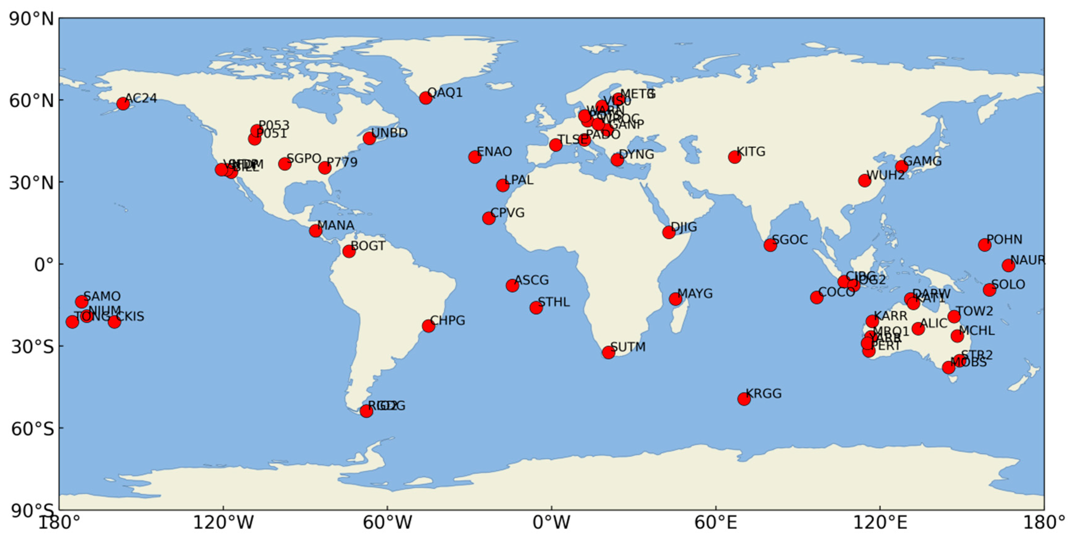
3.1. Observation Dataset

According to the IGS official website, the MGEX tracking station network has exceeded 300 stations worldwide. However, due to differences in receiver types and firmware versions, while many of the MGEX stations can receive BDS-3 and Galileo signals, only some stations can receive the 5 frequencies of BDS-3 and Galileo at the same time. Observation data from 60 MGEX tracking stations were selected, covering a 10-day span from DOY (day of year) 275 to 284 in 2024 (i.e., from 1 October to 10 October 2024). Figure 1 shows the geographical distribution of the selected stations with their BDS-3 and Galileo tracking capabilities and their 5 supported frequencies. Some geographical locations have more stations, while others have fewer stations. The density of the station network is determined by 60 stations, not by the authors’ choice.

These stations are equipped with JAVAD, LEICA, SEPT, STONEX, and TRIMBLE receivers. There are 10 JAVAD receivers, which are controlled by firmware versions JAVAD TRE_3S, JAVAD TRE_3, and JAVAD TRE_3 DELTA. There are 2 LEICA receivers; 1 is controlled by firmware version LEICA GR30, and the other is controlled by LEICA GR50. There are 34 SEPT receivers, which are controlled by firmware versions SEPT POLARX5, SEPT POLARX5TR, SEPT POLARX5S, and SEPT ASTERX4. Only 1 station operates a STONEX receiver, the firmware version of which is STONEX SC2200. Finally, there are 13 TRIMBLE receivers, which are controlled by firmware version TRIMBLE ALLOY. The detailed information of the 60 MGEX tracking stations is shown in

Table 2. Detailed information on the 60 MGEX tracking stations.

Receiver Brand	Site Name	Receiver	Number
JAVAD	SGPO00USA	JAVAD TRE_3S	1
	ENAO00PRT,POTS00DEU,SGOC00LKA,SUTM00ZAF,WUH200CHN	JAVAD TRE_3	5
	BOGT00COL,MET300FIN,STHL00GBR,WARN00DEU	JAVAD TRE_3 DELTA	4
LEICA	WROC00POL	LEICA GR30	1
	LPAL00ESP	LEICA GR50	1
SEPT	AC2400USA,ALIC00AUS,BILL00USA,CKIS00COK,COCO00AUS,DARW00AUS,DJIG00DJI,DYNG00GRC,JOG200IDN,KARR00AUS,KAT100AUS,KITG00UZB, MANA00NIC,METG00FIN,MOBS00AUS,NAUR00NRU,NIUM00NIU,P05100USA,P05300USA,P77900USA,POHN00FSM,QAQ100GRL,SAMO00WSM,SFDM00USA,SOLO00SLB,TONG00TON,TOW200AUS,VIS000SWE,VNDP00USA,YAR300AUS,YARR00AUS	SEPTPOLARX5	31
	GAMG00KOR	SEPT POLARX5TR	1
	UNBD00CAN	SEPT POLARX5S	1
	RIO200ARG	SEPT ASTERX4	1
STONEX	PADO00ITA	STONEX SC2200	1
TRIMBLE	ASCG00SHN, CHPG00BRA,CIBG00IDN,CPVG00CPV,GANP00SVK,KRGG00ATF, MAYG00MYT,MCHL00AUS,MRO100AUS,PERT00AUS,RGDG00ARG,STR200AUS,TLSE00FRA	TRIMBLE ALLOY	13

. Please refer to Appendix A for the detailed performance of all receivers.

3.2. Processing Strategy

All of the PPP experiments were performed with the open-source Net_Diff software developed by the GNSS Analysis Center at the Shanghai Astronomical Observatory (SHAO) [53,54], which can be freely accessed through the webpage http://202.127.29.4/shao_gnss_ac/Net_diff/Net_Diff.rar (accessed on 1 November 2024), version number V1.17.

The satellite orbit and clock bias products used for the PPP calculation in this study were provided by the Deutsches GeoForschungs Zentrum (GFZ), and daily multi-GNSS DCBs were provided by the Chinese Academy of Science (CAS). The coordinate parameters for the static PPP solution were estimated as constants, while they were estimated as white noise on an epoch-by-epoch basis in kinematic mode. Both solutions used Kalman filtering. The PPP processing strategy was based on the default configuration [54], and the processing parameters are summarized in

Table 3. Detailed information on the PPP processing parameters.

Item	Strategies
PPP modes	BDS-3 Standalone, Galileo Standalone
Frequencies	BDS-3: B1C/B2a, B1C/B3I, B1I/B2b, and B1I/B3I; Galileo: E1/E5, E1/E6, E1/E5a, and E1/E5b,
Parameter adjustment	Kalman filter
Troposphere	Zenith: GPT2w. Mapping function: VMF1. The residual part estimated as a random walk parameter.
Ionosphere	Ionosphere-free combination
Satellite phase center offset	Corrected using the European Space Agency (ESA) model
Receiver phase center offset	Corrected by IGS antenna model
Satellite orbit and clock	Precise product of GFZ’s GBM
Daily DCB	CAS’s DCB product
Station displacement	Corrected according to IERS 2010 conventions
Phase windup effect	Corrected
Elevation mask	10°
Station coordinates	Estimated white noise for kinematic mode; constant parameters for static mode.
Receiver clock	Estimated as white noise
Cycle slip detection	GF+MW
Phase ambiguities	Float for BDS-3 and Galileo

. The cycle slip detection adopted a strategy based on dual-frequency Melbourne–Wübbena (MW) and geometry-free (GF) combinations. Due to the use of DFIF combinations, the first-order effects of ionospheric delay were eliminated, and high-order ionospheric delay error entered the unmodeled noise. The troposphere delay was corrected using the Saastamoinen model and the GPT2_5w and VMF1 models [55], and the residual zenith wet delays were estimated. The carrier phase ambiguity was not fixed and remained in a floating-point solution state. It remained constant in continuous arc segments and was reinitialized when a cycle jump occurred. For the determination of specific random models [56] and numerical values, please refer to reference [54].

4. Results

To investigate the DFIF PPP performance of BDS-3 and Galileo in static and kinematic modes, the IGS daily solutions in the Solution Independent Exchange (SINEX) format were adopted as the external reference coordinates. The coordinate differences between the reference solution and the processed ITRF2020 coordinates of the 60 MAGX stations were transformed into north, east, and up (NEU) absolute coordinates.

Due to the fact that a 24 h dataset in static mode only calculates one set of results, the initialization time of PPP was not considered. In kinematic mode, a set of results was calculated at each epoch. The kinematic results calculated in this study were those obtained after PPP initialization was completed.

4.1. Static Results

Because each data segment was 1 day in length and not further segmented in static mode, there was no need to consider the PPP convergence time. Therefore, this study only statistically analyzed the results of the last epoch. For each BDS-3 and Galileo combination, we ultimately obtained 600 solutions from 60 stations over 10 days in static mode.

The daily root mean square error (RMSE) obtained from the static PPP runs of the 60 stations over the period from DOY 275 to DOY 284 in 2024 utilizing BDS-3 and Galileo signals are shown in Figure 2 and Figure 3. The results in Figure 2 and Figure 3 are presented in two decimal places for ease of presentation. The bars are the mean RMSE over all 60 stations for 1 day in Figure 2 and Figure 3.

Figure 2 shows that the PPP performance in static mode remained quite stable for BDS-3’s B1C/B2a, B1C/B3I, B1I/B2b, and B1I/B3I DFIF combinations over 10 days. The results are rounded to two valid decimal places. The maximum daily RMSE differences in the B1C/B2a PPP solutions over 10 days were 0.12 cm, 0.17 cm, and 0.39 cm for the NEU components, respectively. B1C/B3I showed differences of 0.12 cm, 0.14 cm, and 0.27 cm for the NEU components, respectively. B1I/B2b showed differences of 0.10 cm, 0.16 cm, and 0.23 cm for the NEU components, respectively. B1I/B3I showed differences of 0.07 cm, 0.10 cm, and 0.22 cm for the NEU components, respectively.

Figure 3 shows that the PPP performance in static mode maintained stability for Galileo’s E1/E5, E1/E6, E1/E5a, and E1/E5b DFIF combinations over 10 days. The maximum daily RMSE differences in the E1/E5 PPP solutions over 10 days were 0.06 cm, 0.10 cm, and 0.25 cm for the NEU components, respectively. E1/E6 showed differences of 0.08 cm, 0.32 cm, and 0.16 cm, respectively. E1/E5a showed differences of 0.07 cm, 0.12 cm, and 0.21 cm, respectively. E1/E5b showed differences of 0.08 cm, 0.11 cm, and 0.27 cm, respectively.

To present the results of the experiment with more detail, the RMSEs of the static PPP results for BDS-3 and Galileo at each station are shown in Figure 4 and Figure 5, respectively. The sequences of the station names on the horizontal axes of Figure 4 and Figure 5 are arranged alphabetically, and the vertical axis represents different linear combinations.

In Figure 4, it can be seen that the static PPP results of the BDS-3-only DFIF combinations at stations in different geographical locations stations are different. The accuracy in both the east and north directions is better than that in the up direction. It can be seen that some stations experience an up-direction RMSE of about 2.5 cm and perform poorly. The north direction error is smaller than the east direction error, but the difference is not significant among the four DFIF combinations of BDS-3.

In Figure 5, it can be seen that the static PPP results of the Galileo-only DFIF combinations at stations in different geographical locations are different. The accuracy in both the east and north directions is better than that in the up direction. It can be seen that compared to BDS-3, only the SGPO station has an RMSE close to 2.5 cm. For the Galileo E1/E6 combination, the north direction error is significantly smaller than the east direction error, but the other three combinations of Galileo do not show significant differences.

To demonstrate the PPP accuracy in detail, statistical analysis was conducted on the PPP results from all 60 stations over 10 days for both BDS-3 and Galileo in static mode.

Table 4. The RMSE values of the 8 DFIF PPP combinations in static mode. The results were calculated over a period of 10 days (unit: cm).

GNSS	DFIF	RMSE
		N	E	U	H	3D
BDS-3	B1C/B2a	0.47	0.48	1.26	0.67	1.43
	B1C/B3I	0.41	0.42	0.99	0.59	1.15
	B1I/B2b	0.37	0.43	1.02	0.57	1.17
	B1I/B3I	0.37	0.39	1.11	0.54	1.24
Galileo	E1/E5	0.27	0.31	0.98	0.41	1.06
	E1/E6	0.35	0.61	1.01	0.70	1.24
	E1/E5a	0.32	0.31	1.35	0.45	1.42
	E1/E5b	0.23	0.31	1.28	0.39	1.34

shows the RMSE values of the BDS-3 and Galileo DFIF PPP results for the 60 stations over 10 days in static mode, as well as the RMSEs in both the horizontal (H) and three-dimensional (3D) directions.

Table 4 shows that all eight BDS-3 and Galileo signal combinations in static mode show the best accuracy in the north direction, followed by the east direction, and the worst accuracy in the up direction. This is consistent with the conclusion of the original research results. When comparing the different DFIF combinations, one can see that the PPP accuracy of Galileo E1/E5 is the best. The RMSEs of the Galileo E1/E5 combination in the NEU and 3D directions are 0.27 cm, 0.31 cm, 0.98 cm, and 1.06 cm, respectively. The horizontal direction of Galileo E1/E5b performed the best, with an error of 0.39 cm, but its vertical error reached 1.28 cm. The east direction accuracy and north direction accuracy for the five combinations of B1C/B2a, B1C/B3I, B1I/B3I, E1/E5, and E1/E5a are not significantly different.

When a 3D error is used as the evaluation criterion, the order of the combinations from best to worst is as follows: E1/E5, B1C/B3I, B1I/B2b, E1/E6, B1I/B3I, E1/E5b, E1/E5a, and B1C/B2a. However, the accuracy of these eight combinations is similar, with no significant difference, and the RMSEs range between 1.0 and 1.5 cm in static mode. Due to the influence of high-order ionospheric errors, tropospheric residuals, and multipath errors on the positioning accuracy of different combinations, the RMSE values in Table 4 are not fully correlated with the noise amplification factors in Table 1.

4.2. Kinematic Results

The PPP results in kinematic mode had to be statistically analyzed after convergence. The PPP convergence time depends on the number of available satellites, the geometry of the satellites, and the environmental conditions of the reception of the GNSS observations [57]. PPP usually requires 30 min of initialization time. According to the existing literature, there are many criteria for determining whether PPP converges [25,50,51,57]. This study adopted the criteria of reference [58], where the positioning deviation in the NEU directions of the coordinates is considered acceptable when it is less than the predefined threshold value. In this investigation, the threshold value for filter convergence was set to 10 cm. The positioning deviation after the filtering solution stabilized (2 h after the filtering started in this study) was selected to calculate the positioning accuracy [58].

The time series of the average RMSEs for the 60 stations, covering the period from DOY 275 to DOY 284 in 2024 and calculated from BDS-3 and Galileo signals in kinematic mode, are shown in Figure 6 and Figure 7. The results in Figure 6 and Figure 7 are presented in two decimal places for ease of presentation. The bars are the mean RMSE over all 60 stations for 1 day in Figure 6 and Figure 7.

Figure 6 shows that the PPP performance in kinematic mode remained stable for BDS-3’s B1C/B2a, B1C/B3I, B1I/B2b, and B1I/B3I DFIF combinations over 10 days. The maximum daily RMSE differences in the B1C/B2a PPP solutions over 10 days were about 0.62 cm, 0.65 cm, and 0.54 cm for the north, east, and up components, respectively. B1C/B3I showed differences of 0.54 cm, 0.65 cm, and 0.48 cm, respectively. B1I/B2b showed differences of 0.48 cm, 0.53 cm, and 0.54 cm, respectively. B1I/B3I shows differences of 0.47 cm, 0.57 cm, and 0.45 cm, respectively.

Figure 7 shows that the PPP performance in kinematic mode remained stable in Galileo’s E1/E5, E1/E6, E1/E5a, and E1/E5b DFIF combinations over 10 days. The maximum daily RMSE differences in the E1/E5 PPP solutions over the 10 days were 0.21 cm, 0.33 cm, and 0.14 cm for the NEU components, respectively. E1/E6 showed differences of 0.26 cm, 0.42 cm, and 0.27 cm, respectively. E1/E5a showed differences of 0.19 cm, 0.33 cm, and 0.36 cm, respectively. E1/E5b showed differences of 0.24 cm, 0.46 cm, and 0.39 cm, respectively.

To present the results of the experiment, the RMSEs of the kinematic PPP results for BDS-3 and Galileo at each station are shown in Figure 8 and Figure 9, respectively.

In Figure 8, it can be seen that the kinematic PPP results for the BDS-3-only DFIF combinations at stations in different geographical locations are also different. The accuracy in both the east and north directions is better than that in the up direction. It can be seen that one or two stations have up-direction errors of about 5 cm and perform poorly. The north direction error is smaller than the east direction error, but the difference is not significant among the four DFIF combinations for BDS-3.

In Figure 9, it can be seen that the kinematic PPP results of the Galileo-only DFIF combinations at stations in different geographical locations are also different. The accuracy in both the east and north directions is better than that in the up direction. It can be seen that some stations have up-direction errors of about 5 cm and perform poorly. The north direction errors are smaller than the east direction errors, but the differences are not significant among the four Galileo DFIF combinations.

In Figure 4, Figure 5, Figure 8 and Figure 9, it can be seen that the accuracies of the different BDS-3 and Galileo DFIF combinations are correlated in the static and kinematic modes. Due to the fact that PPP accuracy is mainly related to measurement errors and the geometric distribution of satellites, the measurement errors of different DFIF combinations are different. However, the geometric distribution of satellites depends on the number of visible satellites and their relative geometric distribution to the stations. For the same station, the geometric distribution of satellites in different DFIF combinations is almost the same; therefore, the PPP accuracies of different DFIF combinations are also related. Similarly to static mode analysis, in order to demonstrate the PPP accuracy in detail, statistical analysis was conducted on the PPP results from all 60 stations over 10 days for BDS-3 and Galileo in kinematic mode.

Table 5. The RMSE values of the 8 BDS-3 and Galileo DFIF PPP combinations in kinematic mode. The results were calculated over a period of 10 days (unit: cm).

GNSS	DFIF	RMSE
		N	E	U	H	3D
BDS-3	B1C/B2a	1.55	2.13	3.65	2.64	4.50
	B1C/B3I	1.57	2.17	3.69	2.68	4.56
	B1I/B2b	1.45	2.13	3.53	2.58	4.37
	B1I/B3I	1.48	2.08	3.58	2.55	4.40
Galileo	E1/E5	1.42	1.89	3.38	2.36	4.13
	E1/E6	1.85	2.85	3.96	3.40	5.22
	E1/E5a	1.41	1.90	3.46	2.37	4.19
	E1/E5b	1.44	1.92	3.48	2.40	4.23

shows the averages and standard deviations of the RMSE values in kinematic mode. Simultaneously, we calculated the RMSE average values in both the H and 3D directions.

Table 5 shows that in kinematic mode, all eight BDS-3 and Galileo signal combinations showed the best accuracy in the north direction, followed by the east direction, and the worst accuracy in the up direction. When comparing the different DFIF combinations, one can see that the PPP accuracy of the Galileo E1/E5 was the best. The RMSEs of the Galileo E1/E5 combination in the NEU and 3D directions are 1.28 cm, 1.71 cm, 3.25 cm, and 3.59 cm., respectively. The horizontal direction of the Galileo E1/E5 and E1/E5a combinations performed the best, with an error of 2.14 cm. The east direction accuracy and north direction accuracy of the five combinations of B1C/B2a, B1C/B3I, B1I/B3I, E1/E5, and E1/E5a are not significantly different. Compared to the east and up directions, the standard deviation of the north direction has a smaller value, indicating that the accuracy in the north direction is relatively more stable. When the 3D error is used as the evaluation criterion, the order of the combinations in kinematic mode from best to worst is as follows: E1/E5, E1/E5a, E1/E5b, B1I/B2b, B1I/B3I, B1C/B2a, B1C/B3I, and E1/E6. The RMSEs for the 3D PPP of the eight combinations, in the above order, are 3.89 cm, 3.96 cm, 4.00 cm, 4.11 cm, 4.16 cm, 4.27 cm, 4.33 cm, and 4.95 cm, respectively. The best E1/E5 combination was about 1 cm better than the worst E1/E6 combination. The RMSE of the E1/E6 combination reaches about 5.0 cm, while the other seven combinations are approximately 4.0 cm in kinematic mode. Similarly, due to the influence of high-order ionospheric errors, tropospheric residuals, and multipath errors on the positioning accuracy of different combinations, the RMSE values in Table 5 are not fully correlated with the noise amplification factors in Table 1.

5. Discussion

It is not unusual that the RMSEs in the up direction are larger (by a factor of 2–3) than the east and north RMSEs, as all GNSS positioning techniques show this effect. This is due to the satellite/receiver geometry and the correlation between the up component and the parameters of tropospheric delay and clock bias estimate in the PPP model. It is also common for the RMSE in the north direction to be smaller than in the east direction, as the underlying PPP is based on float PPP. The east component stabilizes when ambiguities can be fixed, which is usually achieved through the undifferenced and uncombined PPP ambiguity resolution (PPP-AR) model [24].

Ionospheric delay, which is a critical error mainly generated by signal refraction during propagation and affects GNSS positioning precision, stability, and continuity, should be carefully processed in areas with a sophisticated and active ionosphere [59]. The higher-order error terms, when not accounted for, can degrade the accuracy of GNSS positioning, depending on the level of solar activity and geomagnetic and ionospheric conditions [60]. This study used a conventional DFIF model to eliminate the influence of first-order ionospheric delay and did not consider high-order terms as random errors. However, at high ionospheric activities, higher-order ionospheric errors can reach a few centimeters [61]. Therefore, more sophisticated GNSS ionospheric error correction models [60,62,63,64] should be further considered and discussed.

6. Conclusions

This study analyzed the PPP static and kinematic performance of BDS-3’s B1C/B2a, B1C/B3I, B1I/B2a, and B1I/B3I signal combinations, as well as Galileo’s E1/E5, E1/E6, E1/E5a, and E1/E5b signal combinations, for a total of eight different DFIF combinations. Observation data collected at 60 MGEX stations over 10 days were used to achieve the various PPP combinations.

In this study, the main objective was the evaluation of the eight DFIF combinations’ positioning accuracies in BDS-3-only and Galileo-only systems. The main results and conclusions are summarized as follows:

(1)

The PPP DFIF combinations of BDS-3 are competitive with those of Galileo. Both BDS-3 and Galileo can achieve independent PPP globally in static and kinematic modes.

(2)

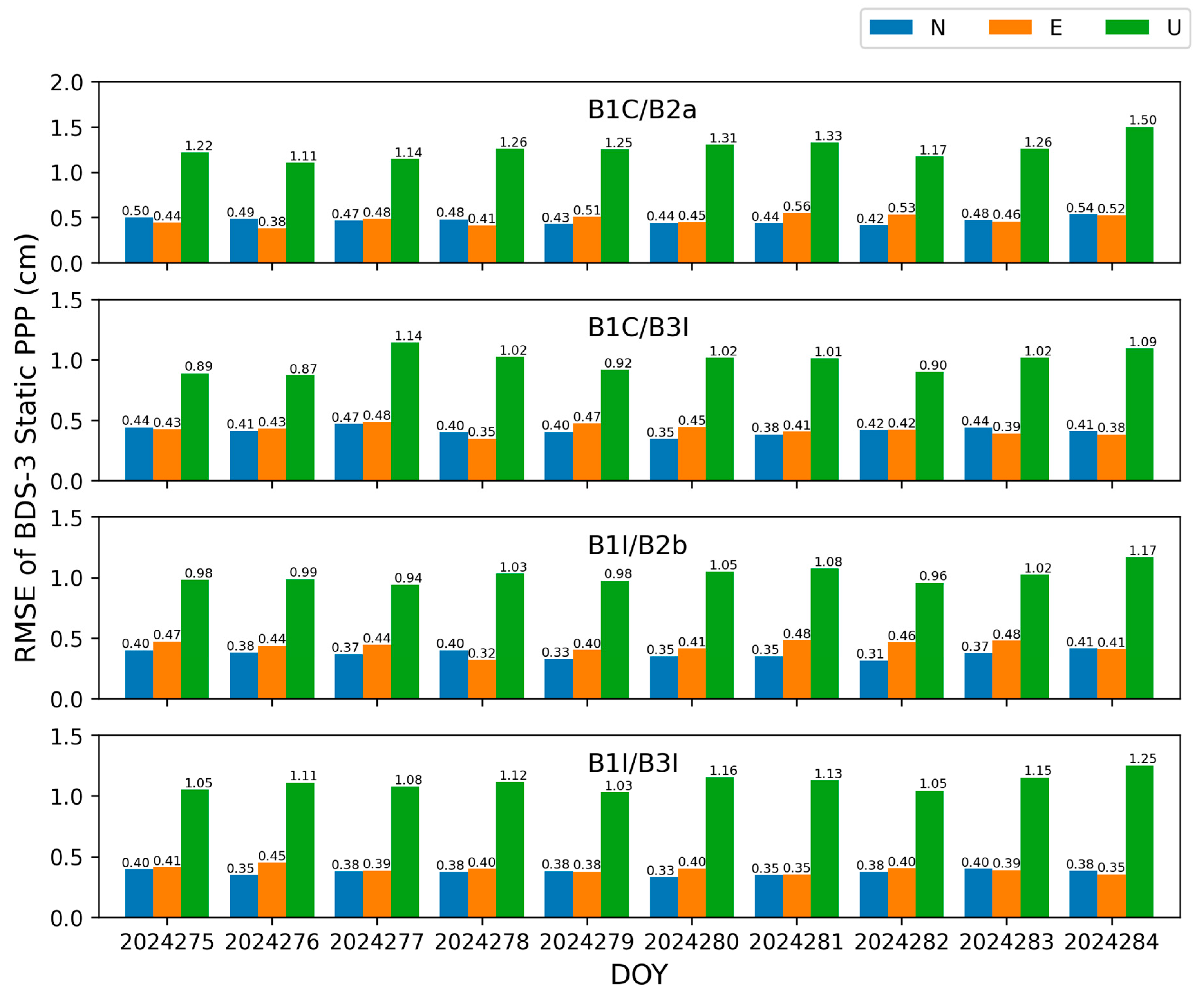
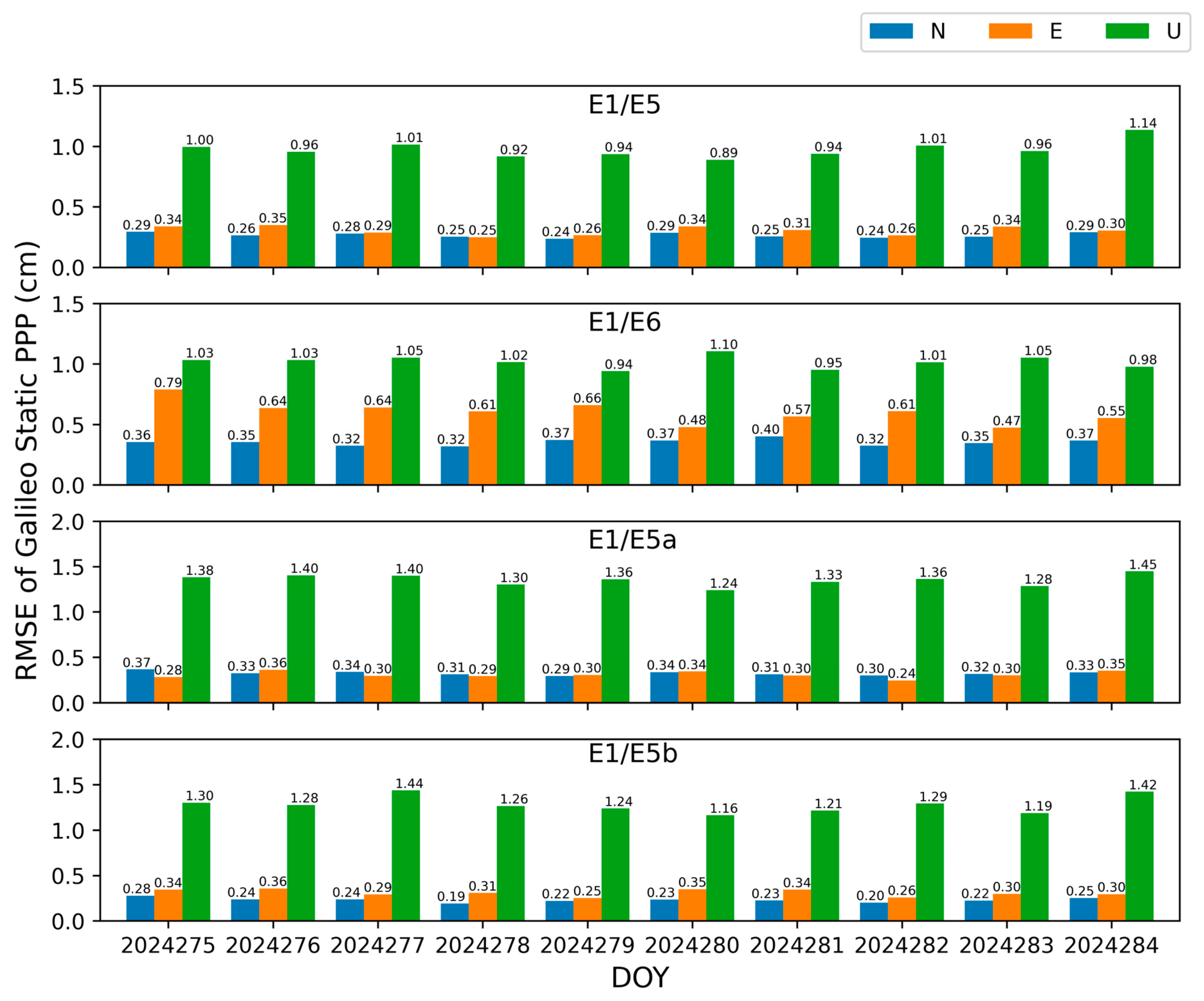
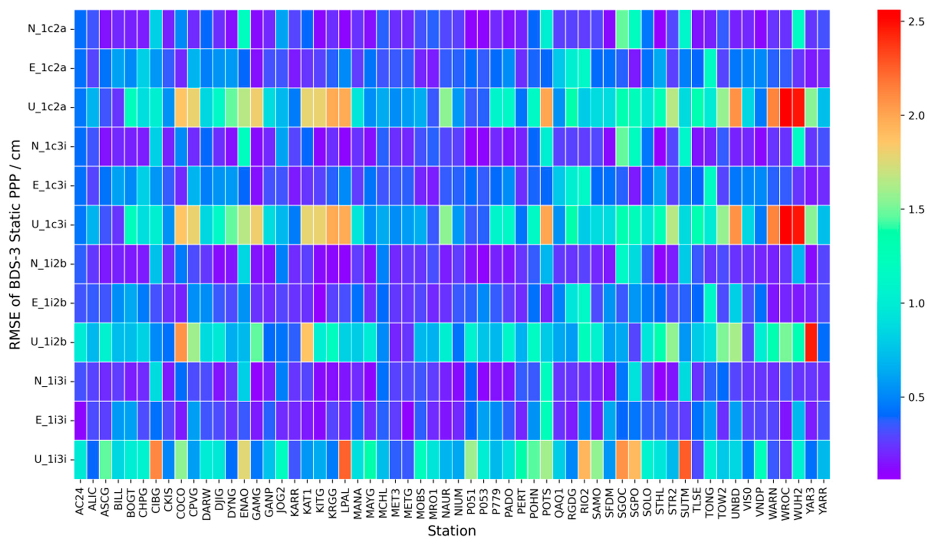
Among the four combinations of BDS-3-only, B1C/B3I showed the best performance in PPP accuracy, with an RMSE of the NEU components of 0.41 cm, 0.42 cm, and 0.99 cm, respectively. B1C/B2a performed the worst, with an RMSE of the NEU components of 0.47 cm, 0.48 cm, and 1.26 cm, respectively, in static mode. Among the four combinations of Galileo-only, E1/E5 showed the best performance in PPP accuracy, with the RMSE of the NEU components being 0.27 cm, 0.31 cm, and 0.98 cm, respectively; E1/E5a performed the worst, with the RMSE of the NEU components being 0.32 cm, 0.31 cm, and 1.35 cm, respectively, in static mode.

When the 3D error is used as the evaluation criterion, the following inequalities summarize the PPP performances of the different DFIF combinations of BDS-3-only and Galileo-only systems in static mode: E1/E5> B1C/B3I> B1I/B2b> E1/E6> B1I/B3I> E1/E5b> E1/E5a > B1C/B2a. The RMSEs of the 3D PPP of the eight combinations, in the above order, are 1.06 cm, 1.15 cm, 1.17 cm, 1.24 cm, 1.24 cm, 1.34 cm, 1.42 cm, and 1.43 cm, respectively. There was no significant difference in the PPP accuracy among the eight combinations, and the positioning accuracy was consistently at the level of 1 cm in static mode.

(3)

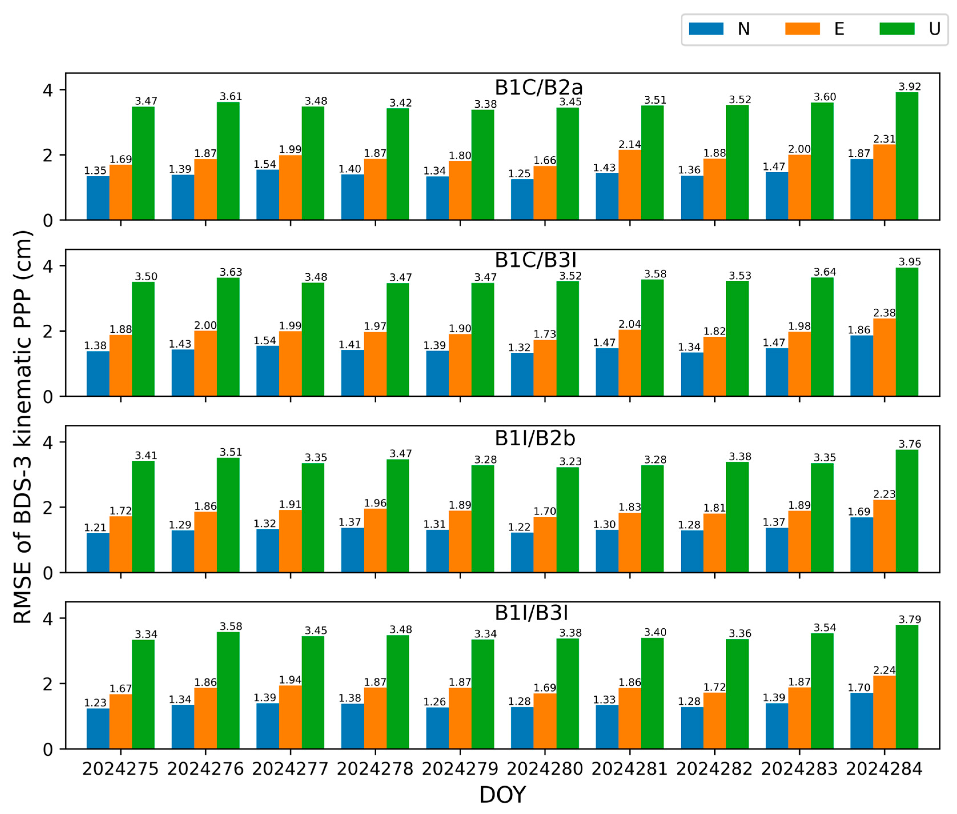
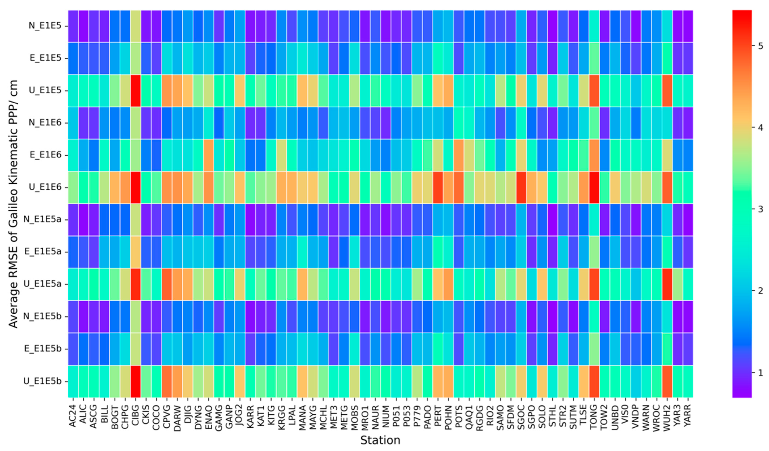
Similarly to the analysis of static mode, among the four BDS-3-only combinations, B1I/B2b showed the best performance in PPP accuracy, with the RMSE of the NEU components being 1.34 cm, 1.88 cm, and 3.40 cm, respectively. B1C/B2a performed the worst, with the RMSE of the NEU components being 1.44 cm, 1.92 cm, and 3.53 cm, respectively, in kinematic mode. Among the four Galileo-only combinations, E1/E5 showed the best performance in PPP accuracy, with the RMSE of the NEU components being 1.28 cm, 1.71 cm, and 3.25 cm, respectively. E1/E6 performed the worst, with the RMSE of the NEU components being 1.70 cm, 2.60 cm, and 3.85 cm, respectively, in kinematic mode.

Using the 3D error as the standard, the following inequalities summarize the PPP performances of the different DFIF combinations of BDS-3-only and Galileo-only systems in kinematic mode: E1/E5 > E1/E5a > E1/E5b > B1I/B2b > B1I/B3I > B1C/B2a > B1C/B3I > E1/E6. The RMSEs for the 3D PPP of the eight combinations, in the above order, were 3.89 cm, 3.96 cm, 4.00 cm, 4.11 cm, 4.16 cm, 4.27 cm, 4.33 cm, and 4.95 cm, respectively. The best E1/E5 combination was about 1 cm better than the worst E1/E6 combination in kinematic mode.

References

1. Rebeiz, G.M. RF MEMS: Theory, Design, and Technology; Wiley: New York, NY, USA, 2003. [Google Scholar]
2. Titterton, D.H.; Weston, J.L. Strapdown Inertial Navigation Technology; Aerospace & Electronic Systems Magazine IEEE; The Institution of Engineering and Technology: Stevenage, UK, 2004. [Google Scholar] [CrossRef]
3. Suvorkin, V.; Garcia-Fernandez, M.; González-Casado, G.; Li, M.; Rovira-Garcia, A. Assessment of Noise of MEMS IMU Sensors of Different Grades for GNSS/IMU Navigation. Sensors 2024, 24, 1953. [Google Scholar] [CrossRef] [PubMed]
4. Shi, J.; Ouyang, C.; Huang, Y.; Peng, W. Assessment of BDS-3 Global Positioning Service: Ephemeris, SPP, PPP, RTK, and New Signal. GPS Solut. 2020, 24, 81. [Google Scholar] [CrossRef]
5. Rovira-Garcia, A.; Juan, J.M.; Sanz, J.; Gonzalez-Casado, G. A Worldwide Ionospheric Model for Fast Precise Point Positioning. IEEE Trans. Geosci. Remote Sens. 2015, 53, 4596–4604. [Google Scholar] [CrossRef]
6. Odolinski, R.; Teunissen, P.J.G.; Odijk, D. Combined BDS, Galileo, QZSS and GPS Single-Frequency RTK. GPS Solut. 2015, 19, 151–163. [Google Scholar] [CrossRef]
7. Teunissen, P.J.G.; Odolinski, R.; Odijk, D. Instantaneous BeiDou+GPS RTK Positioning with High Cut-off Elevation Angles. J. Geod. 2014, 88, 335–350. [Google Scholar] [CrossRef]
8. He, X.; Zhang, X.; Tang, L.; Liu, W. Instantaneous Real-Time Kinematic Decimeter-Level Positioning with BeiDou Triple-Frequency Signals over Medium Baselines. Sensors 2015, 16, 1. [Google Scholar] [CrossRef] [PubMed]
9. Zumberge, J.F.; Heflin, M.B.; Jefferson, D.C.; Watkins, M.M.; Webb, F.H. Precise Point Positioning for the Efficient and Robust Analysis of GPS Data from Large Networks. J. Geophys. Res. 1997, 102, 5005–5017. [Google Scholar] [CrossRef]
10. Malys, S.; Jensen, P.A. Geodetic Point Positioning with GPS Carrier Beat Phase Data from the CASA UNO Experiment. Geophys. Res. Lett. 1990, 17, 651–654. [Google Scholar] [CrossRef]
11. Ge, M.; Gendt, G.; Rothacher, M.; Shi, C.; Liu, J. Resolution of GPS Carrier-Phase Ambiguities in Precise Point Positioning (PPP) with Daily Observations. J. Geod. 2008, 82, 389–399. [Google Scholar] [CrossRef]
12. Aginiparthi, A.S.; Vankadara, R.K.; Mokkapati, R.K.; Panda, S.K. Evaluating the Single-Frequency Static Precise Point Positioning Accuracies from Multi-Constellation GNSS Observations at an Indian Low-Latitude Station. J. Appl. Geod. 2024, 18, 699–707. [Google Scholar] [CrossRef]
13. Cai, C.; Gao, Y. Modeling and Assessment of Combined GPS/GLONASS Precise Point Positioning. GPS Solut. 2013, 17, 223–236. [Google Scholar] [CrossRef]
14. Yue, C.; Dang, Y.; Xue, S.; Wang, H.; Gu, S.; Xu, C. A New Optimal Subset Selection Method of Partial Ambiguity Resolution for Precise Point Positioning. Remote Sens. 2022, 14, 4819. [Google Scholar] [CrossRef]
15. Pan, Y.; Geng, J.; Liu, K.; Chen, X.; Fang, R. Evaluation of Rapid Phase Clock/Bias Products for PPP Ambiguity Resolution and Its Application to the M7.1 2019 Ridgecrest, California Earthquake. Adv. Space Res. 2020, 65, 2586–2594. [Google Scholar] [CrossRef]
16. Kim, H.; Hyun, C.-U.; Park, H.-D.; Cha, J. Image Mapping Accuracy Evaluation Using UAV with Standalone, Differential (RTK), and PPP GNSS Positioning Techniques in an Abandoned Mine Site. Sensors 2023, 23, 5858. [Google Scholar] [CrossRef] [PubMed]
17. Goudarzi, M.A.; Banville, S. Application of PPP with Ambiguity Resolution in Earth Surface Deformation Studies: A Case Study in Eastern Canada. Surv. Rev. 2018, 50, 531–544. [Google Scholar] [CrossRef]
18. Meng, X.; Wang, J.; Han, H. Optimal GPS/Accelerometer Integration Algorithm for Monitoring the Vertical Structural Dynamics. J. Appl. Geod. 2014, 8, 265–272. [Google Scholar] [CrossRef]
19. Guo, J.; Li, X.; Li, Z.; Hu, L.; Yang, G.; Zhao, C.; Fairbairn, D.; Watson, D.; Ge, M. Multi-GNSS Precise Point Positioning for Precision Agriculture. Precis. Agric. 2018, 19, 895–911. [Google Scholar] [CrossRef]
20. Zhang, X.; Li, P.; Zuo, X. Kinematic Precise Orbit Determination Based on Ambiguity-Fixed PPP. Geomat. Inf. Sci. Wuhan Univ. 2013, 38, 1009–1013. [Google Scholar]
21. Grayson, B.; Penna, N.T.; Mills, J.P.; Grant, D.S. GPS Precise Point Positioning for UAV Photogrammetry. Photogramm. Record. 2018, 33, 427–447. [Google Scholar] [CrossRef]
22. Zhang, B.; Ou, J.; Yuan, Y.; Li, Z. Extraction of Line-of-Sight Ionospheric Observables from GPS Data Using Precise Point Positioning. Sci. China Earth Sci. 2012, 55, 1919–1928. [Google Scholar] [CrossRef]
23. Zhang, F.; Tang, L.; Li, J.; Du, X. A Simple Approach to Determine Single-Receiver Differential Code Bias Using Precise Point Positioning. Sensors 2023, 23, 8230. [Google Scholar] [CrossRef] [PubMed]
24. Geng, J.; Bock, Y. Triple-Frequency GPS Precise Point Positioning with Rapid Ambiguity Resolution. J. Geod. 2013, 87, 449–460. [Google Scholar] [CrossRef]
25. Lou, Y.; Zheng, F.; Gu, S.; Wang, C.; Guo, H.; Feng, Y. Multi-GNSS Precise Point Positioning with Raw Single-Frequency and Dual-Frequency Measurement Models. GPS Solut. 2016, 20, 849–862. [Google Scholar] [CrossRef]
26. Afifi, A.; El-Rabbany, A. Performance Analysis of Several GPS/Galileo Precise Point Positioning Models. Sensors 2015, 15, 14701–14726. [Google Scholar] [CrossRef]
27. Li, P.; Jiang, X.; Zhang, X.; Ge, M.; Schuh, H. GPS + Galileo + BeiDou Precise Point Positioning with Triple-Frequency Ambiguity Resolution. GPS Solut. 2020, 24, 78. [Google Scholar] [CrossRef]
28. Chen, C.; Xiao, G.; Chang, G.; Xu, T.; Yang, L. Assessment of GPS/Galileo/BDS Precise Point Positioning with Ambiguity Resolution Using Products from Different Analysis Centers. Remote Sens. 2021, 13, 3266. [Google Scholar] [CrossRef]
29. Hou, Z.; Zhou, F. Assessing the Performance of Precise Point Positioning (PPP) with the Fully Serviceable Multi-GNSS Constellations: GPS, BDS-3, and Galileo. Remote Sens. 2023, 15, 807. [Google Scholar] [CrossRef]
30. Li, X.; Ge, M.; Dai, X.; Ren, X.; Fritsche, M.; Wickert, J.; Schuh, H. Accuracy and Reliability of Multi-GNSS Real-Time Precise Positioning: GPS, GLONASS, BeiDou, and Galileo. J. Geod. 2015, 89, 607–635. [Google Scholar] [CrossRef]
31. Liu, T.; Yuan, Y.; Zhang, B.; Wang, N.; Tan, B.; Chen, Y. Multi-GNSS Precise Point Positioning (MGPPP) Using Raw Observations. J. Geod. 2017, 91, 253–268. [Google Scholar] [CrossRef]
32. Zhou, F.; Cao, X.; Ge, Y.; Li, W. Assessment of the Positioning Performance and Tropospheric Delay Retrieval with Precise Point Positioning Using Products from Different Analysis Centers. GPS Solut. 2020, 24, 12. [Google Scholar] [CrossRef]
33. Li, M.; Qu, L.; Zhao, Q.; Guo, J.; Su, X.; Li, X. Precise Point Positioning with the BeiDou Navigation Satellite System. Sensors 2014, 14, 927–943. [Google Scholar] [CrossRef] [PubMed]
34. Guo, F.; Zhang, X.; Wang, J.; Ren, X. Modeling and Assessment of Triple-Frequency BDS Precise Point Positioning. J. Geod. 2016, 90, 1223–1235. [Google Scholar] [CrossRef]
35. Xia, F.; Ye, S.; Xia, P.; Zhao, L.; Jiang, N.; Chen, D.; Hu, G. Assessing the Latest Performance of Galileo-Only PPP and the Contribution of Galileo to Multi-GNSS PPP. Adv. Space Res. 2019, 63, 2784–2795. [Google Scholar] [CrossRef]
36. Liu, S.; Zhu, S.; Zhang, J. Investigating Performance of BDS-2+3 Dual-Frequency Absolute Positioning With Broadcast Ephemerides, RTS and Final MGEX Products. IEEE Access 2023, 11, 22034–22050. [Google Scholar] [CrossRef]
37. China Satellite Navigation Office. Available online: http://www.beidou.gov.cn/ (accessed on 1 November 2024).
38. China Satellite Navigation Office. BeiDou Navigation Satellite System Signal in Space Interface Control Document Open Service Signal B1I (Version 3.0). Available online: http://www.beidou.gov.cn/xt/gfxz/201902/P020190227593621142475.pdf (accessed on 1 November 2024).
39. China Satellite Navigation Office. BeiDou Navigation Satellite System Signal in Space Interface Control Document Open Service Signal B1C (Version 1.0). Available online: http://www.beidou.gov.cn/xt/gfxz/201712/P020171226741342013031.pdf (accessed on 1 November 2024).
40. China Satellite Navigation Office. BeiDou Navigation Satellite System Signal in Space Interface Control Document Open Service Signal B2a (Version 1.0). Available online: http://www.beidou.gov.cn/xt/gfxz/201712/P020171226742357364174.pdf (accessed on 1 November 2024).
41. China Satellite Navigation Office. BeiDou Navigation Satellite System Signal in Space Interface Control Document Open Service Signal B2b (Version 1.0). Available online: http://www.beidou.gov.cn/xt/gfxz/202008/P020230516558683155109.pdf (accessed on 1 November 2024).
42. China Satellite Navigation Office. BeiDou Navigation Satellite System Signal in Space Interface Control Document Open Service Signal B3I (Version 3.0). Available online: http://www.beidou.gov.cn/xt/gfxz/201802/P020180209623601401189.pdf (accessed on 1 November 2024).
43. European GNSS Service Centre (GSC). Available online: https://www.gsc-europa.eu/system-service-status/constellation-information (accessed on 1 November 2024).
44. The European GNSS (Galileo) Open Service Signal-In-Space Interface Control Document (Issue 2.0). Available online: https://galileognss.eu/wp-content/uploads/2021/01/Galileo_OS_SIS_ICD_v2.0.pdf (accessed on 1 November 2024).
45. Zhou, F.; Dong, D.; Li, W.; Jiang, X.; Wickert, J.; Schuh, H. GAMP: An Open-Source Software of Multi-GNSS Precise Point Positioning Using Undifferenced and Uncombined Observations. GPS Solut. 2018, 22, 33. [Google Scholar] [CrossRef]
46. Collins, P.; Bisnath, S.; Lahaye, F.; Héroux, P. Undifferenced GPS Ambiguity Resolution Using the Decoupled Clock Model and Ambiguity Datum Fixing. Navigation 2010, 57, 123–135. [Google Scholar] [CrossRef]
47. Héroux, P.; Kouba, J. GPS Precise Point Positioning Using IGS Orbit Products. Phys. Chem. Earth Part A Solid Earth Geod. 2001, 26, 573–578. [Google Scholar] [CrossRef]
48. Vankadara, R.; Dashora, N.; Panda, S.K.; Dabbakuti, J.R.K.K. A Comparative Analysis of the Effect of Orbital Geometry and Signal Frequency on the Ionospheric Scintillations over a Low Latitude Indian Station: First Results from the 25th Solar Cycle. Remote Sens. 2024, 16, 1698. [Google Scholar] [CrossRef]
49. Ogutcu, S.; Alcay, S.; Ozdemir, B.N.; Li, P.; Zhang, Y.; Konukseven, C.; Atiz, O.F. Assessing the Performance of BDS-3 for Multi-GNSS Static and Kinematic PPP-AR. Adv. Space Res. 2023, 71, 1543–1557. [Google Scholar] [CrossRef]
50. De Oliveira, P.S.; Morel, L.; Fund, F.; Legros, R.; Monico, J.F.G.; Durand, S.; Durand, F. Modeling Tropospheric Wet Delays with Dense and Sparse Network Configurations for PPP-RTK. GPS Solut. 2017, 21, 237–250. [Google Scholar] [CrossRef]
51. Zhou, F.; Dong, D.; Ge, M.; Li, P.; Wickert, J.; Schuh, H. Simultaneous Estimation of GLONASS Pseudorange Inter-Frequency Biases in Precise Point Positioning Using Undifferenced and Uncombined Observations. GPS Solut. 2018, 22, 19. [Google Scholar] [CrossRef]
52. Misra, P.; Enge, P. Global Positioning System-Signals, Measurements, and Performance; Ganga-Jamuna Press: Kathmandu, Nepal, 2001. [Google Scholar]
53. Zhang, Y.; Kubo, N.; Chen, J.; Wang, J.; Wang, H. Initial Positioning Assessment of BDS New Satellites and New Signals. Remote Sens. 2019, 11, 1320. [Google Scholar] [CrossRef]
54. Zhang, Y.; Chen, J.; Gong, X.; Chen, Q. The Update of BDS-2 TGD and Its Impact on Positioning. Adv. Space Res. 2020, 65, 2645–2661. [Google Scholar] [CrossRef]
55. Böhm, J.; Möller, G.; Schindelegger, M.; Pain, G.; Weber, R. Development of an Improved Empirical Model for Slant Delays in the Troposphere (GPT2w). GPS Solut. 2015, 19, 433–441. [Google Scholar] [CrossRef]
56. Yue, C.; Dang, Y.; Gu, S.; Wang, H.; Zhang, J. Optimization of Undifferenced and Uncombined PPP Stochastic Model Based on Covariance Component Estimation. GPS Solut. 2022, 26, 119. [Google Scholar] [CrossRef]
57. Malik, J.S. Analysis of Position Coordinate Accuracy of Triple GNSS System by Post-Processing Dual Frequency Observations Using Open Source GAMP: A Case Study. Acta Geodyn. Geomater. 2020, 17, 485–499. [Google Scholar] [CrossRef]
58. Zhou, F.; Xu, T. Modeling and assessment of GPS/BDS/Galileo triple-frequency precise point positioning. Acta Geod. Cartogr. Sin. 2021, 50, 61–70. [Google Scholar] [CrossRef]
59. Cheng, S.; Cheng, J.; Zang, N.; Zhang, Z.; Zhao, G.; Chen, S. Stochastic Characteristics Analysis on GNSS Observations and Real-Time ROTI-Based Stochastic Model Compensation Method in the Ionospheric Scintillation Environment. GPS Solut. 2024, 28, 130. [Google Scholar] [CrossRef]
60. Hoque, M.M.; Jakowski, N. Higher Order Ionospheric Effects in Precise GNSS Positioning. J. Geod. 2007, 81, 259–268. [Google Scholar] [CrossRef]
61. Cai, C.; Liu, G.; Yi, Z.; Cui, X.; Kuang, C. Effect Analysis of Higher-Order Ionospheric Corrections on Quad-Constellation GNSS PPP. Meas. Sci. Technol. 2019, 30, 024001. [Google Scholar] [CrossRef]
62. Luo, X.; Li, H.; Gong, X.; Xie, Z.; Li, Y. BDS-3 B1I Signal Tracking Error Characteristic and Its Advantage in PPP Under Ionospheric Scintillation at Low Latitudes. IEEE Trans. Geosci. Remote Sens. 2023, 61, 1–10. [Google Scholar] [CrossRef]
63. Luo, X.; Liu, Z.; Lou, Y.; Gu, S.; Chen, B. A Study of Multi-GNSS Ionospheric Scintillation and Cycle-Slip over Hong Kong Region for Moderate Solar Flux Conditions. Adv. Space Res. 2017, 60, 1039–1053. [Google Scholar] [CrossRef]
64. Zhou, Y.; Kuang, C.; Cai, C. Analysis of Higher-Order Ionospheric Effects on GNSS Precise Point Positioning in the China Area. Surv. Rev. 2019, 51, 442–449. [Google Scholar] [CrossRef]
Figure 1. The distribution of the 60 MGEX stations used in this study.
Atmosphere 16 00316 g001
Figure 2. Time series of static PPP RMSE of BDS-3-only DFIF combinations.
Atmosphere 16 00316 g002
Figure 3. Time series of static PPP RMSE of Galileo-only DFIF combinations.
Atmosphere 16 00316 g003
Figure 4. RMSEs of static PPP results for BDS-3-only DFIF combinations at each station.
Atmosphere 16 00316 g004
Figure 5. RMSEs of static PPP results for Galileo-only DFIF combinations at each station.
Atmosphere 16 00316 g005
Figure 6. Time series of kinematic PPP RMSEs of BDS-3-only DFIF combinations.
Atmosphere 16 00316 g006
Figure 7. Time series of kinematic PPP RMSEs of Galileo-only DFIF combinations.
Atmosphere 16 00316 g007
Figure 8. RMSEs of kinematic PPP results for BDS-3-only DFIF combinations at each station.
Atmosphere 16 00316 g008
Figure 9. RMSEs of kinematic PPP results for Galileo-only DFIF combinations at each station.
Atmosphere 16 00316 g009