Article

Spatio-Temporal Variability in CO2 Fluxes in the Atlantic Sector of the Southern Ocean

by
Gabrielle Tavares de Carvalho
1,
Luciano Ponzi Pezzi
1,*,
Nathalie Lefèvre
2,
Celina Cândida Ferreira Rodrigues
1,
Marcelo Freitas Santini
1 and
Carlos Mejia
2
1
Laboratory of Ocean and Atmosphere Studies (LOA), Earth Observation and Geoinformatics Division (DIOTG), National Institute for Space Research (INPE), Av. dos Astronautas, 1758, São José dos Campos 12227-010, SP, Brazil
2
Laboratoire d’Océanographie et du Climat: Expérimentations et Approches Numériques, Sorbonne Université, Centre National de la Recherche Scientifique (CNRS), Institut de Recherche pour le Developpement (IRD), Museum National d’Histoire Naturelle (MNHN) and Institut Pierre Simon Laplace (IPSL), Place Jussieu, 4, 75252 Paris, France
*
Author to whom correspondence should be addressed.
Atmosphere 2025, 16(3), 319; https://doi.org/10.3390/atmos16030319
Submission received: 5 February 2025 / Revised: 25 February 2025 / Accepted: 28 February 2025 / Published: 10 March 2025

Abstract

:
The Southern Ocean (SO) plays a fundamental role in the planet’s climate system, due to its ability to absorb and redistribute heat and CO2 (an important greenhouse gas). In addition, the SO connects three large oceanic basins the Pacific, the Atlantic, and the Indian Oceans, and it has an important role in the nutrient distribution in these oceans. However, the SO is poorly sampled, with most measurements made in austral spring and summer. The variability in the air–sea CO2 flux is estimated, as well as the role of atmospheric and oceanic variables in this variability. The CO2 fluxes are calculated using the bulk parameterization method, in the Atlantic sector of the Southern Ocean, from 2003 to 2022, using in situ measurements, satellites, and a reanalysis data set. A neural network model is built to produce maps of the partial pressure of CO2 in seawater (pCO2sea). The CO2 flux varies from −0.05 to 0.05 gC m−2 month−1. The Atlantic sector of the SO is a sink of CO2 in summer and spring and becomes a source in austral winter and autumn. The CO2 absorption intensifies from 2003 to 2022 by 7.6 mmol m−2 month−1, due to stronger westerly winds, related to the trend in the positive phase of the Antarctic Oscillation and the extreme El Niño Southern Ocean (ENSO) events (e.g., El Niño and La Niña).

1. Introduction

The Southern Ocean (SO) is considered an important CO2 sink area, with an absorption of −1.0 Pg C/year [1]. The main cause is the cold waters of the region, which result in greater CO2 solubility [2,3]. In the SO, there is an intense transformation and formation of water masses, with a strong seasonality [4] which helps to control oceanic carbon reservoirs [5].
The CO2 flux (FCO2) exchange between the ocean and the atmosphere varies in time and space [6,7]. The oceanic mesoscale may play a crucial role in these flux exchanges. For example, [8] showed that sea surface temperature (SST) anomalies caused by a warm core eddy (WCE) in the Southwestern Atlantic Ocean (SWA), near the SO, exerted a crucial influence on modifying the Marine Atmospheric Boundary Layer (MABL) by transferring heat and CO2 from the ocean to the atmosphere. The WCE presence in midlatitudes, surrounded by predominantly cold waters, caused the ocean to act locally as a CO2 source. Rodrigues et al. (2024) found that the intense horizontal gradient of SST combined with moderate wind and turbulence in the Brazil Malvinas Confluence (BMC) modulates FCO2, leading to a CO2 sink. Seasonal variations are explained by SST variations and biological activity [6,7]. Interannual and decadal variations may be related to changes in deep water formation and are associated with the Antarctic Oscillation (AO) and the El Niño Southern Oscillation (ENSO) [9,10,11]. Nevertheless, the magnitude of the influence of ENSO and AO on FCO2 variability is still not understood [7].
The Eddy Covariance (EC) is a method used to measure the exchange of turbulent energy and mass between the atmosphere and the ocean’s surface and has already been used in previous studies in the Southwestern Atlantic, such as those by [8,12,13], to study the MABL’s stability. The role of roughness and stability on momentum fluxes at Brazil Malvinas Confluence was studied in [14]. Recently, ref. [8] studied the turbulence and instability of the MABL caused by an oceanic WCE and consequent modification in the behavior of CO2, heat, and momentum fluxes in the BMC. Additional information about EC can be found in these cited articles, as the methodology employed in this study is the same.
The El Niño Southern Oscillation (ENSO), despite occurring in equatorial regions, influences the SST variability and the wind field in some regions of the SO, due to Rossby wave propagation. These waves are generated through vorticity from adiabatic heating, which, when moving south, induce teleconnections between ENSO and the SO climate [15,16]. ENSO has a La Niña phase (cold phase) and an El Niño phase (warm phase) [17]. AO is represented by an oscillation in surface pressure systems between medium and high latitudes in the Southern Hemisphere, with positive and negative phases [18]. The Antarctic Oscillation is usually defined as the difference in the zonal mean sea level pressure at 40° S (midlatitudes) and 65° S (Antarctica) [19]).
The positive AO phase is defined by negative anomalies of geopotential height and temperature, in addition to the increase in the strength of the westerlies that lead to a greater upwelling of carbon from the ocean depths to the surface, which reduces the absorption of CO2. The opposite occurs in the negative AO phase [20,21,22]. During El Niño, there is an increase in the mixing of Circumpolar Deep Water (CDW) with Dense Shelf Water (DSW) advected from the Weddell Sea, leading to greater absorption of CO2. The opposite occurs during La Niña [10,11,21,22,23].
The SO location, the high seasonality, and ice cover make it difficult to carry out oceanographic cruises, generating a lack of spatio-temporal information from the existing data set [24,25,26] There are few measurements in autumn and winter; most of them are made in austral summer and spring [16,27,28]. This makes it necessary to use tools that interpolate available measurements.
Here, we use in situ data from the unprecedented collections of the Antarctic Modeling and Observation System (ATMOS), along with scientific insights from both the ATMOS and ATMOS 2 projects. The Surface Ocean CO2 Atlas (SOCAT) (https://www.socat.info, accessed on 1 January 2022) satellite and reanalysis datasets are used to estimate the air–sea CO2 fluxes and their variability from 2003 to 2022. As pCO2sea is not available from satellite data, we built an Artificial Neural Network (ANN) model to produce maps of pCO2sea. ANNs have become an increasingly efficient tool in the field of CO2 studies and have been applied in estimations of pCO2sea and CO2 fugacity [1,29,30] In addition, they perform better than linear regressions [30].
Thus, this study contributes to increasing our knowledge of the spatio-temporal variability in the FCO2 in the Atlantic sector of the Southern Ocean, as well as the role of atmospheric and oceanic variables in explaining this variability. From this, it becomes possible to understand the causes of the intensification of the CO2 absorption, as well as the consequences for the studied region.
We organize this article as follows: Section 2 describes the methodology and the data. Section 3 provides the main results found in this study. Section 4 discusses the analysis carried out and presents the conclusions and final remarks of this work.

2. Materials and Methods

The study area is presented in Section 2.1, followed by in situ data (Section 2.2) related to the ATMOS Project satellite and reanalysis data set (Section 2.3). Direct measurements of CO2 fluxes obtained from the ATMOS oceanographic cruise are described in Section 2.4. The training of the neural network based on the ATMOS and SOCAT data sets is described in Section 2.5. The CO2 flux data estimated from the bulk parameterization are described in Section 2.6. Finally, the FCO2 variability analysis technique is described in Section 2.7.

2.1. Study Area

The SO has the largest and fastest ocean current on the globe, the Antarctic Circumpolar Current (ACC), driven by the strong easterly winds’ characteristic of southern polar latitudes [31,32,33]. The oceanic circulation of the SO occurs as follows: the upper cell of the meridional circulation is driven by wind, which causes upwelling of the CDW along inclined isopycnals, due to divergent Ekman transport, which upwell in the ACC [34]. At the surface, CDWs become Subantarctic Modal Waters (SMWs) and Antarctic Intermediate Waters (AIWs), which constitute the upper part of the Southern Overturning Circulation [35]. Surface buoyancy flows, ocean–atmosphere interactions, ice shelves, and sea ice produce cold, salty Dense Shelf Water (DSW). DSW becomes the dense Antarctic Bottom Water (ABW), formed in seas such as the Ross and Weddell Seas, and along the east coast of Antarctic [36].
When the ACC reaches the Drake Passage, the narrowing between the Antarctica Peninsula and the southern edge of South America causes an increase in the ACC speed, and results in the strengthening of the main circumpolar oceanic fronts present in the region (Figure 1). These fronts, from south to north, are as follows: (1) the Southern Boundary (BF), which is the northern limit of the cold water mass; (2) the Southern Antarctic Circumpolar Current Front (SACCF), which extends approximately along the Antarctic slope and deviates slightly northwards at 56° W; (3) the Polar Front (PF), formed by the convergence of Antarctic and subantarctic waters, and (4) the Subantarctic Front (SAF) which defines the northern boundary of the ACC. To the north of the SAF is the Subtropical Front (STF), which marks the northernmost extent of subantarctic waters [31].
Around Antarctica there is a cover of sea ice, which varies seasonally. It reduces during the warm season, due to melting (minimum in February), and during the cold season it expands, due to freezing (maximum in September) [15,16]. In addition to the aforementioned factors that can affect the FCO2, there is also the passage of atmospheric cold fronts. Indeed, the fronts cause changes in the surface wind field, pressure, temperature, and other atmospheric variables during their trajectory, in addition to their interactions with the sea surface [37].

2.2. In Situ Data

In situ data were obtained from the ATMOS project (Table 1). The oceanographic cruise occurred during OPERANTAR XL, aboard Brazilian Navy Polar Vessel (Po/V) Almirante Maximiano (H-41), between November 2021 and February 2022 [8,38]. The data were collected by sensors installed in the meteorological tower at the bow of the ship, and data were measured by LI-COR (LI-850) installed in one laboratory of the ship (Table 1). The data are available in [39].
The sea surface salinity (SSS) data were interpolated from reprocessing systems that combine data from NASA’s Soil Moisture Active Passive (SMAP) and European Space Agency’s (ESA’s) Soil Moisture Ocean Salinity (SMOS) satellites and in situ measurements (https://doi.org/10.48670/moi-00051, accessed on 5 May 2023). The sea surface temperature (SST) data are from the reprocessing of Along Track Scanning Radiometer (ATSR), Sea and Land Surface Temperature Radiometer (SLSTR), and Advanced Very High Resolution Radiometer (AVHRR) satellite data by the ESA SST Climate Change Initiative (CCI) and Climate Change Service (C3S) projects; they were produced from the Operational Sea Surface Temperature and Sea Ice Analysis system (OSTIA) (https://doi.org/10.48670/moi-00169, accessed on 10 May 2023).
SSS, SST, sea level pressure (SLP), H2O density, and partial pressure of CO2 gas in the sea (pCO2sea) were obtained from SOCAT. Interpolated Air temperature (Tair) and wind speed were obtained from the MERRA-2 satellite (https://disc.gsfc.nasa.gov/datasets/M2TMNXAER_5.12.4/summary?keywords=merra2, accessed on 15 May 2023). Interpolated concentrations of CO2 (xCO2air) were downloaded from Global View (https://gml.noaa.gov/about/aboutgml.html, accessed on 20 May 2023) pCO2air is the partial pressure of CO2 in the atmosphere. The pCO2air was obtained from xCO2air, Patm, and pH2O [1].

2.3. Satellite and Reanalysis Data Set

A collection of satellites and a reanalysis data set were used for the study of the Atlantic sector of the SO and for the FCO2 estimation. The FCO2 estimation was made using a data set from satellite multiple sources to extend and complete the time series for the period from 2003 to February 2022.
The satellite data used in this study are described here. The CO2 estimates used are from the Atmospheric Infrared Sounder (AIRS) sensor, on board the Aqua satellite, with a spatial resolution of 2.5° × 2°, at the equator from 2003 to 2014 (https://disc.gsfc.nasa.gov/datasets/AIRX3C2M_005/summary?keywords=AIRX3C2M_005, accessed on 7 May 2023). The 2015 to 2022 CO2 estimates are from the Orbiting Carbon Observatory-2 (OCO-2) satellite, which provides estimations with a spatial resolution of 0.5° × 0.625°km (https://disc.gsfc.nasa.gov/datasets/OCO2_GEOS_L3CO2_MONTH_10r/summary?keywords=oco-2, accessed on 7 May 2023). The SLP, Tair, and wind speed were obtained from the Modern-Era Retrospective analysis for Research and Applications, Version 2 (MERRA-2) satellite, with spatial resolution of 0.5° × 0.625°, from 2003 to 2022.
Monthly reanalyses of the SST and SSS were obtained from Multi Observation Global Ocean ARMOR3D (https://doi.org/10.48670/moi-00052, accessed on 15 May 2023). These analyses combine satellite data from Advanced Very High Resolution Radiometer (AVHRR) and Advanced Microwave Scanning Radiometer-2 (AMSR-2), and in situ observations distributed by NOAA’s National Climatic Data Center, with a spatial resolution of 0.25° × 0.25°, from 2003 to 2022.
The chlorophyll products used in this work are from of PISCES biogeochemical model of two ocean modeling platforms (NEMO and CROCO), three Earth System models (IPSL-CM, CNRM-CM and EC-Earth) and one operational oceanographic system (MERCATOR-Ocean) (https://data.marine.copernicus.eu/product/GLOBAL_MULTIYEAR_BGC_001_029/description, accessed on 20 May 2023), with a spatial resolution of 0.25° × 0.25°, from 2003 to 2022.

2.4. Eddy Covariance Method

Eddy Covariance (EC) is the method used to obtain direct measurements of turbulent fluxes from the covariance between the fluctuations in the mean CO2 density and the vertical component of the wind, thus providing the flux in CO2 between the ocean surface and the atmosphere as indicated in Equation (1) [12,13,40]. These measurements are made at high temporal frequencies and are performed in the surface layer of the Marine Atmospheric Boundary Layer (MABL) [8,41]. The MABL is the layer nearest to the ocean surface, which is where momentum, heat, and gas exchange take place [42].
The FCO2 is given in µmol m−2 s−1, using the fluctuations in the vertical wind component w   (m/s) and the CO2 density c (m·gm−3), in relation to their averages denoted by the overbar, the dry air density ρ a (kg·m), and the average molecular weight of carbon dioxide (CO2), which is 44.01 g·mol−1:
FCO 2 =   ρ a   w c ¯
The calculation of the FCO2 was performed using the free open-source software EddyPro® v7.0.9, offered by LI-COR Biosciences Inc. (Omaha, NE, USA) (EddyPro v7.0.9). Fluxes are calculated using a 30 min average of high-frequency (20 Hz) data. Before the FCO2 calculation, the wind data were corrected due to the ship’s movement [3,43].

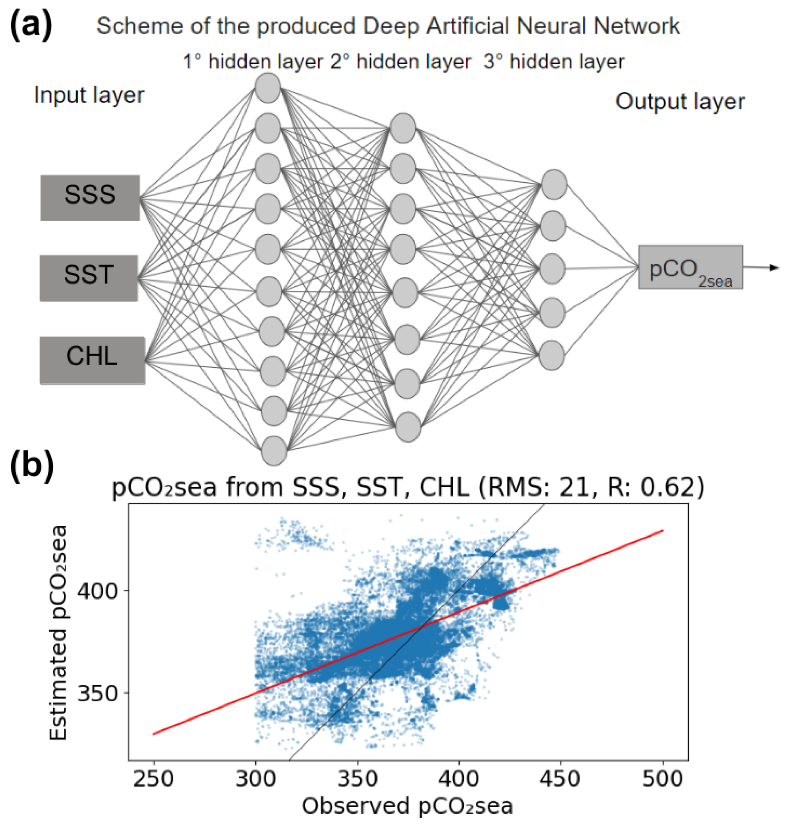
2.5. Artificial Neural Network to Estimate pCO2sea

The ocean CO2 partial pressure (pCO2sea) data are very sparse in the study area. Therefore, an Artificial Neural Network (ANN) was used to fill spatial and temporal gaps in pCO2sea [1]. In this study, 279.480 observations from SOCAT and ATMOS over the 2003–2022 period were used to reconstruct the pCO2sea for the study region. The data set was split into two distinct groups [44]:
(1) A total of 85% of the data were randomly selected for utilization during the training phase. This is identified as the Train set.
(2) The remaining 15% were allocated to the neural network diagnosis phase. This is called the Test set.
The standard procedure of data normalization (scaling) was implemented on every input and output variable, aiming to achieve a mean of 0 and a standard deviation of 1 for each of them. The network consists of an input layer composed of 3 neurons, 3 hidden layers with 10, 8, and 5 nodes, respectively, and an output layer, that is, the estimate of pCO2sea, as shown in Figure 2. For the precision analysis of the pCO2sea estimate, the mean squared error and Pearson’s coefficient were defined [44]. Previous studies that applied this methodology to the Atlantic Ocean used SST, SSS, and chlorophyll [1]. Therefore, in this study, these variables were also used as input for the ANN model to estimate pCO2sea (Figure 2a). Thus, it was possible to obtain a moderate correlation between the reference data and the estimates produced by the ANN, based on Pearson’s correlation, R = 0.62, and with a root mean square error (RMS) of 21 (Figure 2b). The scatter observed in Figure 2 is due to the great variability in the input parameters of the ANN in the study region. This variability is associated with the frequent passage of atmospheric transient systems that modify the ocean surface, strong SST gradients due to the mixing of water masses of different origins, and variations in SSS and chlorophyll caused by precipitation and freshwater input from different rivers.
The model was produced in the Python 3 programming language, available in public repository and referred in section “Data Availability Statement”. Two platforms were also installed: TensorFlow and Keras [45]. The ANN estimated pCO2sea. With pCO2sea, it was then possible to calculate FCO2 on a large spatial and temporal scale.

2.6. Bulk Parameterization

FCO2 was determined by the bulk parameterization (FCO2BK) shown in Equation (2), where FCO2BK is defined by the product of the ocean–atmosphere CO2 partial pressure gradient ∆pCO2 (∆pCO2= pCO2sea − pCO2air), the solubility (s), and the wind-dependent air–sea gas transfer velocity (K) [46,47]:
FCO2BK = s·k·∆pCO2(sea−air)
The solubility (s) of CO2 in seawater was defined with the relationship used by [48]. The k was calculated according to [49] using monthly mean wind speed. The direction and part of the magnitude of FCO2 are defined by ΔpCO2, whose variability is dominated by pCO2sea in our observations.
The bulk parameterization was applied using satellite and reanalysis data from 2003 to 2022. However, each data source used in this study has a different spatial resolution from the others, so it was necessary to remap them (Table 2). The interpolation was based on the spatial resolution of CO2 observations from the AIRS and OCO-2 satellites. From 2003 to 2014, the data had a final spatial resolution of 2° × 2.5°, and from 2015 to 2022 the final spatial resolution was 0.5° × 0.625°. The interpolation was performed using the “nearest neighbor” algorithm through the NumPy library of the Python 3 tool. This tool was used due to its simplicity of application and to ensure that the interpolated value is one of the original values [50]. For each location to be interpolated, the distances from all sample points to that same location are calculated and, from this, the corresponding interpolation value is the value of the smallest distance observed [50].

2.7. CO2 Flux Variability Analysis

The analysis of FCO2 in the Drake Passage covered the month of February in the years 2016 and 2019 based on bulk SOCAT data, and from 1 December 2021 to 15 February 2022, based on the ATMOS project collections [3,8,38] obtained with the EC method.
Afterwards, the bulk was applied again, but now with satellite data, reanalysis, and ANN, in the Atlantic sector of the Southern Ocean. Next, an analysis of the monthly FCO2 series was carried out and the role of atmospheric and oceanic variables in FCO2 variability was described. The influence of ENSO and AO on FCO2 was also investigated. ENSO and AO information is available from the Climate Prediction Center (CPC), the National Oceanic and Atmospheric Administration (NOAA), and the National Center for Environmental Prediction (NCEP) during the period from 2003 to February 2022.

3. Results

In this section, we present the results of this study, based on in situ data collection, estimated fluxes, and reanalysis data, in addition to flux estimates resulting from the Artificial Neural Network model calculations.

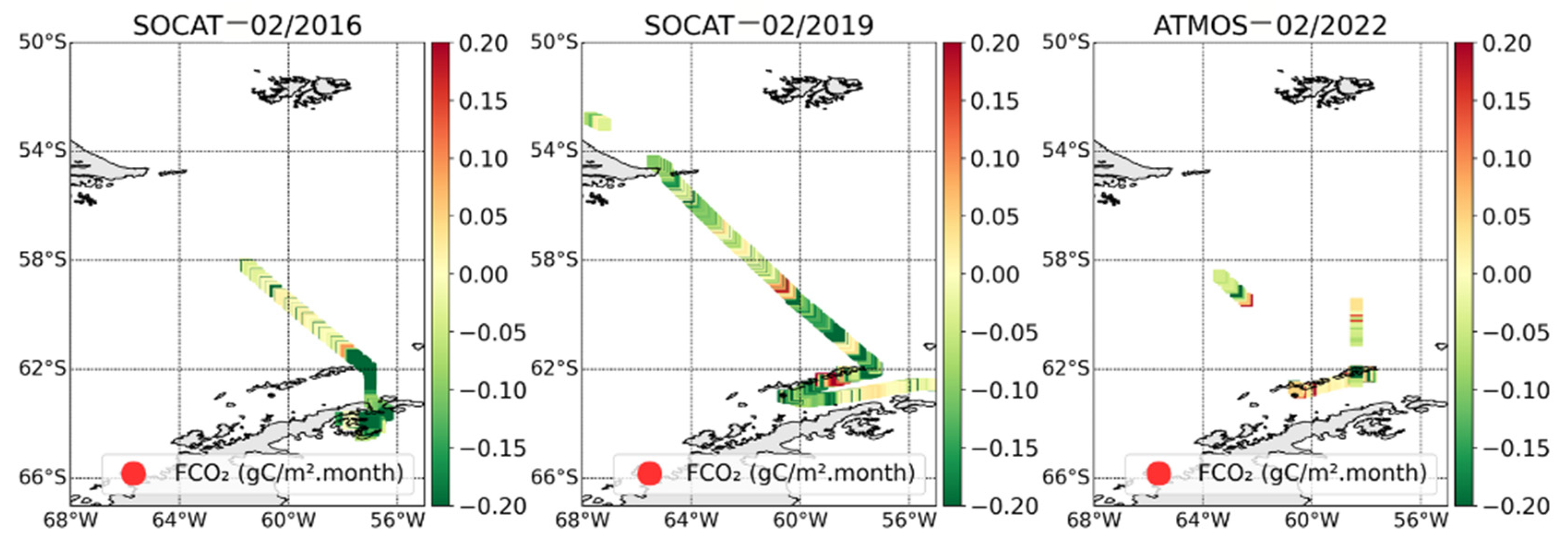
3.1. CO2 Flux Variability in February

The monthly FCO2 in the Drake Passage is presented for February 2016, 2019, and 2022 (Figure 3). Using bulk parameterization with SOCAT data, the values were −0.01 gC m−2 month−1 in 2016 and −0.005 gC m−2 month−1 in 2019. Using EC with ATMOS data in 2022, the flux was −0.04 gC m−2 month−1. The negative flux observed by both data sets indicates the behavior of CO2 absorption by the ocean, which was also observed by Takahashi et al. (2009), who in their study also obtained a negative FCO2 of −0.02 gC m−2 month−1. These values are due to the Southern Ocean acting as a CO2 sink during austral summer [10,28,51]. This absorption in the summer occurs because it is a period of increased availability of light and nutrients. Nutrients are from upwelled Circumpolar Deep Waters (CDWs), which leads to an increase in phytoplankton blooms, a decrease in the pCO2sea, and an increase in CO2 uptake by the ocean [9,52,53]. Despite the predominance of CO2 absorption in the Drake Passage, there was a release of CO2 near 60° S observed with SOCAT and ATMOS data in 2019 and 2022 (Figure 3).

3.2. FCO2 Calculated with an Artificial Neural Network

The 2003–2022 average FCO2, calculated from the maps of pCO2sea, was −0.027 gC m−2 month−1, and from in situ data the average was −0.029 gC m−2 month−1, but the average bias is small (−0.002 gC m−2 month−1). FCO2 from in situ data (SOCAT and ATMOS data) was determined with the bulk method from 2003 to 2022. The comparison between the two fluxes can be seen in the Taylor diagram, which provides a simple graphical representation of what the next one will bring from the other (Figure 4). In relation to the standard deviation of the observed data, it was 2.4 and that of the model was 1.7 (Figure 4). The root mean square error (RMS) error between the two was 1.5. The FCO2, based on the reconstruction of pCO2sea, may have overestimated the flux variability by 5.3%. However, this underestimation is low, in comparison with data reported by [54] for the Southern Ocean, at 31%. The percentage overestimation is, by definition, inversely proportional to the standard deviation of the model [54]. The correlation with the flux calculated with in situ data was high (r = 0.76), and was higher than that observed in [54] with r = 0.54.
To detect possible increases or decreases in CO2 absorption, we calculate the monthly CO2 flux anomalies over 2003–2022 using the maps produced by the ANN (Figure 5).
The area from 40° S to 45° S exhibits large seasonal changes with positive flux in the months of December, January, and February (austral summer) and in the months of September, October, and November (austral spring), and negative values in the months of June, July, and August (austral winter) and in March, April, and May (austral autumn). The region from 45° S to 55° S also exhibits seasonal changes, ranging from being a strong sink of CO2 in summer and spring and having reduced absorption in winter and autumn, indicating that it is a year-round sink. This region is the Antarctic Divergence area, located within the high-wind-speed zone (40° S–60° S). The strong winds cause a large vertical mixing of seawater, which increases the exchange of CO2 at the air–sea interface, explaining the strong CO2 sink [55,56]. In this region, the North Atlantic Deep Water resurfaces from a 2000 m depth to 200 m, with higher temperatures [57]. South of 55° S is an area of year-round CO2 absorption. However, absorption is reduced in winter and autumn. During the southern spring–summer, phytoplankton blooms occur near the sea ice and increase the CO2 absorption. This indicates the effect of reduced sea ice cover on the FCO2 in this region, as observed in [24,28,58].
In summer, absorption is more intense than in other seasons (Figure 5), with 72% more absorption than in autumn and winter, and 51% more than in the southern spring. The absorption peak occurs mainly in February; this is due, in part, to the reduction in surface salinity caused by the seasonal melting of sea ice, which makes the ocean more soluble. The lowest absorption values are mainly in August due to increased salinity from the release of salt during the formation of sea ice and high-density water that will sink with the CO2-rich waters. The expansion of sea ice cover occurs in autumn and winter, with maximum extension in August and September. Also, during this period, the ocean can even become a source of CO2 for the atmosphere, caused by high salinity values at the surface that cause a reduction in the solubility of CO2 in the ocean [15,16]. The ice cover can extend from the Antarctic continent to 55° S in the Atlantic sector in some years; however, on average it can extend up to 62° S in winter [24]. As winter progresses, ice formation increases, releasing salts, which can contribute to the release of CO2 into the water. The layer of mixed water under the ice is rich in CO2, mainly due to the vertical mixing of deep waters [24,59]. However, in the summer and spring the ice cover melts and reaches its minimum size in February, which is why this is the month in which the greatest absorption of CO2 occurs [60]. Furthermore, in the southern summer and spring there is an increase in light availability and stable stratification of surface water, which allows an increase in primary biological productivity, which leads to an increase in CO2 absorption during these seasons [9,52,53].
The FCO2 varies from −0.05 to 0.05 gC m−2 month−1 in the Atlantic sector of the SO, with increased absorption in the summer and spring periods, and in the southern winter and autumn, absorption decreases. CO2 absorption has intensified in the study area, with an increase of 0.076 gC m−2 month−1 from 2003 to 2022. This behavior is shaped by wind speed and SST, but mainly by the intensification of winds that increased during the studied period, which may be driven by climate variability [10,34,61]. Furthermore, an increasing trend in pCO2air was also observed, which has shown increasingly higher levels than in water. The increase in pCO2air is due to anthropogenic CO2 emissions. The rate of increase of pCO2sea is slower in highly mixed regions as deeper waters with a lower CO2 content are brought to the surface. In highly stratified regions, the same rate of increase is observed in the ocean and in the atmosphere. Previous studies that modeled future scenarios already expected this response from the Southern Ocean to increased CO2 emissions [62,63,64,65,66]. These models predicted that in scenarios with high greenhouse gas emissions, there would be a reduction in the efficiency of absorption by the ocean. This occurs because the increase in atmospheric CO2 concentration is linked to the increase in anthropogenic emissions [67]. Thus, although absorption by the ocean has intensified, the ocean is not able to absorb all the excess CO2 present in the atmosphere resulting from anthropogenic emissions.
In the Drake Passage, the absorption in the summer and spring periods is of −0.01 gC m−2 month−1 and −0.013 gC m−2 month−1, respectively. In the autumn and winter periods, there is a reduction in absorption of −0.012 gC m−2 month−1. Similar results were observed by Takahashi et al. (2009). In summer and spring, they observed strong CO2 absorption, and in autumn and winter there is a reduction in absorption, namely −0.09 gC m−2 month−1, −0.02 gC m−2 month−1, 0.01 gC m−2 month−1, and 0.013 gC m−2 month−1, respectively.
The SST anomaly maps produced using reanalysis data, shown in Figure 6, illustrate that some regions of the study area are becoming increasingly warmer over time, which affects FCO2. The waters coming from the Pacific Ocean through the Drake Passage to the Atlantic sector of the Southern Ocean are releasing more CO2 than the expected average (Figure 5). These are the waters from the PF. The PF is located approximately at latitude 50° S in the Atlantic and at latitude 60° S in the Pacific. This is a region where CO2 is released, due to its average surface temperature being higher than that south of this region. This behavior was also observed with SOCAT and ATMOS data as shown in Figure 3. The surface water south of this region moves northwards and sinks when it reaches the PF, thus causing convergence at the surface [68]. However, with the increase in SST, the PF shows stronger CO2 outgassing. To the north of the PF there is an increase in CO2 release; this region has higher temperatures, due to the dominant effect of seasonal SST changes [57]. However, to the south of the PF there is an increase in CO2 absorption. In this region, the surface waters of the Antarctic Zone have very low temperatures, reaching values close to the freezing point (−1.9 °C), as a result of the summer melting of the sea ice and surface cooling in winter [57]. Below the surface in the Antarctic Zone, extending up to 4000 m deep, is the Antarctic Circumpolar Water (AACW), with temperatures of 1.5 to 2.5 °C [57]. Close to the coast of the Antarctic continent, some regions also intensified the release of CO2. Despite being a region with a higher potential temperature than at the shelf break, the SST was also warmer. This region is where the Deep Circumpolar Water rises over the slope to enter the platform, as it has warmer and saline waters [69]. However, the waters that are a source of CO2 are expanding southward, and the waters that are sinks of CO2 become stronger sinks. This is due to the increase in strength and southward displacement of the westerly winds, associated with the positive trend in the AO, which forces the migration of the FS towards the Antarctic continent, thus migrating warm and saline waters, which cause the release of CO2. This trend towards the positive phase of OA is due to the increase in greenhouse gases [18,34,70].

3.3. Variability in CO2 Flux

In the region between 63° W and 54° W and 59° S to 62° S, in the Drake Passage, an analysis of the temporal variability of FCO2 and atmospheric and oceanic variables was carried out, including the climate indices ENSO and OA, based on the historical series from 2003 to 2022.
The physical pumping of CO2 from the atmosphere to the ocean is associated with the solubility of CO2 in water, which is influenced by changes in temperature, salinity, and atmospheric pressure, in addition to the action of winds, since wind speed influences absorption [55]. Thus, it was possible to observe the variation in FCO2 because of changes in the variables used in this study. There is a tendency towards negative CO2 values throughout the period studied (Figure 7a), with peaks and decreasing values, which follows the seasonality of the SST (Figure 7b). The SLP varies inversely to the temperature, that is, when the temperature increases the SLP decreases and vice versa (Figure 7b,e). Furthermore, the SLP appears to be inversely proportional to the FCO2, so it is possible to observe that where there is a drop in the SLP, there is an increase in the values of FCO2, which become more positive (Figure 7e). This relationship between SLP and FCO2 indicates a decrease in the concentration of atmospheric CO2 near the surface and, consequently, there is a tendency to transfer CO2 from the ocean to the atmosphere. Wind speed is strongest in the months of March to November, ranging from 11 to 13 (m/s), and reduces in the months of December to February (southern summer), ranging from 9 to 10 (m/s) (Figure 7g). Biological CO2 pumping is carried out by photosynthetic activity, and the analysis in this study was based on CHL, which varies seasonally. CHL blooms occur during the austral spring–summer and decrease in the austral autumn–winter (Figure 7c). The months of August and September have the lowest concentrations of CHL.
It was observed from ΔpCO2 (Figure 7d), which defines the direction and part of the magnitude of FCO2, that pCO2air is what dominates the variability in FCO2 in this study. ΔpCO2 has a decreasing trend, indicating that the direction of FCO2 is towards the ocean. An increasing trend in pCO2air was also observed (Figure 7h), which has been increasingly higher than in pCO2sea. The increase in pCO2air may be caused by the high concentration of anthropogenic CO2 present in the air, which is not being captured by the ocean with the same efficiency as before. Previous studies that simulated future scenarios already expected this response from the SO to increased CO2 emissions [63,64,65,66,67]. These models predicted that in scenarios with high greenhouse gases emissions, there would be a reduction in the efficiency of absorption by the ocean. The weakening of CO2 absorption by the SO is due to the existence of a natural limit in gas exchange at the atmosphere–ocean interface, CO2 dissociation, turbulent mixing, and ocean circulation, which causes only a certain percentage of excess CO2 atmospheric pressure to be absorbed. Therefore, although oceanic absorption is increasing, there are still high concentrations of CO2 in the atmosphere [9,56,71].
CO2 absorption increased by 0.076 gC m−2 month−1 from 2003 to 2022. Winds were intense, averaging 11.1 m/s (Figure 7g). The SST was higher than the air temperature (SST > Tair) throughout the studied period (Figure 7b), which indicates that the Marine Atmospheric Boundary Layer (MABL) in this region is unstable and that an intense exchange of CO2 occurs, as suggested by [8,72].
The months May 2005, May 2007, June 2009, June 2011, July 2019 and July 2021 had absorption anomalies (FCO2 varying from 0.075 gC m−2 month−1 to 0.2 gC m−2 month−1) (Figure 7a), that is, absorption was more intense in these periods than the expected average. These periods showed that the high negative values of FCO2 were due to high values of SLP (ranging from 1008 hPa to 1013 hPa) and low values of SST (ranging from 8 °C to 10 °C) and Tar (ranging from 4.7 °C to 6.7 °C), as well as intense winds (ranging from 11 m/s to 12.3 m/s), which caused the exchange of CO2 at the ocean surface to be greater, with K varying from 18 to 33. However, in February 2013 (FCO2 0.0134 gC m−2 month−1) CO2 absorption was lower than the expected average due to low SLP values (1006 hPa) and wind speed and warmer SST and Tair, which caused gas transfer at the ocean–atmosphere interface to be lower; the k was 4.8.
Interannual variations are related to the phase variation in OA and ENSO, as observed by [10,11,17,23]. The months when an intense reduction in CO2 absorption occurred, such as February 2013, had the influence of positive OA (+OA). +OA is defined by negative geopotential height and temperature anomalies. +OA increases the strength of westerly winds that lead to an increase in the upwelling of natural carbon from the depths of the ocean to the surface, causing a reduction in CO2 absorption. However, the opposite occurred in the months May 2005, May 2007, June 2009, June 2011, June 2019 and July 2021which had intense CO2 absorption and a period of -OA [20,21,22,73,74]. Furthermore, June 2015, despite being a +OA month, was the most extreme El Niño period since 1998 [28]. In this case, the role of El Niño was greater than that of OA. During El Niño, there is an increase in the mixing of Deep Circumpolar Waters with Dense Shelf Water advected from the Weddell Sea, leading to greater absorption of CO2. The opposite occurs in La Niña [10,11,20,21,22,23,74]. The change in OA phase influences the flux variability, which can increase (negative phase) or reduce (positive phase) the absorption of CO2. ENSO becomes the main influence only in periods of strong intensity, as occurred in 06/2015. Therefore, most of the time the main modulator of FCO2 is OA.

4. Final Remarks and Conclusions

This study showed the spatio-temporal variability in the sea–air FCO2 caused by the ocean and atmosphere conditions in the Atlantic sector of the Southern Ocean. The FCO2, calculated through the EC method using in situ data collected by the ATMOS project [3,8,38], offered a new source of atmospheric and oceanic data for CO2, heat, and momentum in the Atlantic sector of the Southern Ocean.
Monthly maps of FCO2 were produced using an Artificial Neural Network for estimating pCO2sea with satellite and reanalysis data from 2003 to 2022. The absolute error between the FCO2 produced from the ANN and that produced with in situ data was −1.3 μmol m−2 month−1 and the correlation was high (r = 0.9). This corresponds to a slight overestimation of 5.3% compared to the 31% obtained by [54] in the SO.
The FCO2 varies from −0.05 to 0.05 gC m−2 month−1 in the Atlantic sector of the SO, with the strongest CO2 sink occurring in the summer and spring periods, and a lower sink in the austral winter and autumn. The seasonal variation in FCO2 is modulated by changes in SST in the Atlantic sector of the SO. In summer, absorption is more intense than in other seasons, and the peak mainly occurs in February. Summer absorption is 72% greater than that in autumn and winter; and is 51% greater than that in the southern spring. The lowest absorption values occur mainly in August (winter). This is due to the expansion of sea ice cover that occurs in autumn and winter, with maximum expansion in August and September.
From 2003 to 2022, CO2 absorption intensified by 0.076 gC m−2 month−1. In summer, absorption increased by 0.093 gC m−2 month−1 compared to that in 2003 to 2022. In autumn, winter, and spring, the increase was 0.11 gC m−2 month−1, 0.14 gC m−2 month−1, and 0.1 gC m−2 month−1, respectively, from 2003 to 2021.
During the study period, FCO2 varied spatially, shaped by the characteristics of ocean fronts. The areas of the SF, because they have warm and saline waters, act as a source. Areas between the SF and the SAF, characterized by moderate SST and SSS and intense winds, have strong absorption. Finally, there are areas with moderate absorption, located in the regions of the SB, in the SACCF and in the PF, which have colder and less saline waters.
The waters, which act as a source of CO2, are expanding southwards, and the waters, which act as sinks, have been intensifying the absorption of CO2. This is due to the increased strength and southward displacement of the westerly winds, associated with the positive trend in the AO, which forced the migration of the SF towards the Antarctic continent. Thus, warm and saline waters migrate and cause the release of CO2. In addition, the intensification of westerly winds on the circumpolar oceanic fronts intensifies the absorption of CO2 in this region. The influence of ENSO only overlaps with the influence of the OA phase in periods of extreme ENSO, such as what occurred in 2015.
The results of this study show that FCO2 in the SO are highly dependent on oceanographic and atmospheric conditions. The spatial variation in FCO2 is affected by the displacement of water masses. In addition, the intensification of westerly winds in the SAF, which increases gas exchange at the ocean–atmosphere interface, intensifies the absorption of CO2 in this region. It also supports previous studies that simulated future scenarios on the reduction in the efficiency of CO2 absorption by the ocean as a response by the Southern Ocean to the increase in greenhouse gas emissions. The ANN model for pCO2sea estimates is a very important tool to fill data gaps for pCO2sea in difficult-to-access areas, such as the SO, mainly in winter and southern autumn periods. It is also evident that the continuity of in situ sampling in this region with high-quality data will allow us to improve the models produced and improve our understanding of the role of dynamic and thermodynamic processes that act as modulating mechanisms of CO2 fluxes at the ocean–atmosphere interface of the Atlantic sector of the Southern Ocean.

Author Contributions

Conceptualization, G.T.d.C., L.P.P. and N.L.; methodology, G.T.d.C., L.P.P., N.L., M.F.S., C.C.F.R. and C.M.; software, G.T.d.C. and C.M.; validation, G.T.d.C.; formal analysis, G.T.d.C.; investigation, G.T.d.C.; data curation, G.T.d.C., M.F.S. and C.C.F.R.; writing—original draft preparation, G.T.d.C.; writing—review & editing, G.T.d.C., L.P.P., N.L., M.F.S., C.C.F.R. and C.M.; supervision, L.P.P. and N.L. All authors have read and agreed to the published version of the manuscript.

Funding

This research was funded by the Brazilian agencies agency CNPq, through the following projects: (i) Antarctic Modeling and Observation System (CNPq/PROANTAR 443013/2018-7). (ii) The study of the Antarctic Climate, the Southern Ocean, and their relations with the Brazilian and South American environment (ATMOS 2.0) (CNPq/PROANTAR 440848/2023-7). L.P.P. is partly funded through a CNPq Scientific Productivity Fellowship (CNPq/303981/2023-7). This study was financed in part by the Coordenação de Aperfeiçoamento de Pessoal de Nível Superior, Brasil (CAPES)—Finance Code 001.

Institutional Review Board Statement

Not applicable.

Informed Consent Statement

Not applicable.

Data Availability Statement

The Artificial Neural Network (ANN) software was designed to estimate pCO2sea. The ANN used in the article can be found at [75] https://doi.org/10.5281/zenodo.10854860 (accessed on 10 May 2024), and can be developed openly in Python 3. Data from the meteorological tower installed on the bow of the Brazilian Navy Polar Ship (Po/V) Almirante Maximiano (H-41) were used to calculate the CO2 flux (FCO2) in the EddyPro®v7.0.9 software. These available data are in Carvalho, G.T., and Pezzi, L.P., 2024 (https://doi.org/10.5281/zenodo.10871385, accessed on 10 May 2024). LI-COR (LI-850) data installed in the laboratory aft of the Brazilian Navy Polar Ship (Po/V) Almirante Maximiano (H-41) were used to calculate pCO2sea, available in Carvalho and Pezzi (2024) in https://doi.org/10.5281/zenodo.10887055, accessed on 10 May 2024.

Acknowledgments

The authors thank the Brazilian Navy, the Brazilian Ministry of Science, Technology and Innova-tions (MCTI), and the Brazilian Antarctic Program (PROANTAR) for making the ATMOS 2.0 project and cruises possible and enjoyable. The authors also acknowledge the support from the Graduate Program in Remote Sensing (PGSER) from the National Institute for Space Research (INPE).

Conflicts of Interest

The authors declare no conflict of interest.

References

  1. Landschützer, P.; Gruber, N.; Bakker, D.C.E.; Schuster, U.; Nakaoka, S.; Payne, M.R.; Sasse, T.P.; Zeng, J. A neural network-based estimate of the seasonal to inter-annual variability of the Atlantic Ocean carbon sink. Biogeosciences 2013, 10, 7793–7815. [Google Scholar] [CrossRef]
  2. Silva, L.A.; de Andrade, J.B.; Lopes, W.A.; Carvalho, L.S.; Pereira, P.A.P. Solubility and reactivity of gases. Quim. Nova 2017, 40, 824–832. [Google Scholar] [CrossRef]
  3. Rodrigues, C.C.F.; Santini, M.F.; Lima, L.S.; Sutil, U.A.; Carvalho, J.T.; Cabrera, M.J.; Rosa, E.B.; Burns, J.W.; Pezzi, L.P. Ocean-atmosphere turbulent CO2 fluxes at Drake Passage and Bransfield Strait. An. Acad. Bras. Ciências 2023, 95, e20220652. [Google Scholar] [CrossRef] [PubMed]
  4. Santini, M.F.; Souza, R.B.; Wainer, I.; Muelbert, M.M. Temporal analysis of water masses and sea ice formation rate west of the Antarctic Peninsula in 2008 estimated from southern elephant seals’ SRDL–CTD data. Deep Sea Res. Part II Top. Stud. Oceanogr. 2018, 149, 58–69. [Google Scholar] [CrossRef]
  5. Bremer, U.F.; Campos, L.d.S.; Evangelista, H.; Garcia, C.A.E.; Goldemberg, J.; Mata, M.M.; Paulsen, L.; Simões, J.C. Antártica e as Mudanças Globais: Um Desafio para a Humanidade; Blucher: São Paulo, Brazil, 2011; E-book; ISBN 9788521216087. Available online: https://app.minhabiblioteca.com.br/books/9788521216087 (accessed on 20 March 2023).
  6. Landschützer, P.; Gruber, N.; Haumann, F.A.; Rödenbeck, C.; Bakker, D.C.E.; van Heuven, S.; Hoppema, M.; Metzl, N.; Sweeney, C.; Takahashi, T.; et al. The reinvigoration of the Southern Ocean carbon sink. Science 2015, 349, 6253. [Google Scholar] [CrossRef]
  7. Sutton, A.J.; Williams, N.L.; Tilbrook, B. Constraining Southern Ocean CO2 Flux Uncertainty Using Uncrewed Surface Vehicle Observations. Geophys. Res. Lett. 2021, 48, e2020GL091748. [Google Scholar] [CrossRef]
  8. Pezzi, L.P.; de Souza, R.B.; Santini, M.F.; Miller, A.J.; Carvalho, J.T.; Parise, C.K.; Quadro, M.F.; Rosa, E.B.; Justino, F.; Sutil, U.A.; et al. Oceanic eddy-induced modifications to air–sea heat and CO2 fluxes in the Brazil-Malvinas Confluence. Sci. Rep. 2021, 11, 10648. [Google Scholar] [CrossRef]
  9. Heinze, C.; Meyer, S.; Goris, N.; Anderson, L.; Steinfeldt, R.; Chang, N.; Le Quéré, C.; Bakker, D.C.E. The ocean carbon sink—Impacts, vulnerabilities and challenges. Earth Syst. Dynam. 2015, 6, 327–358. [Google Scholar] [CrossRef]
  10. Brown, M.S.; Munro, D.R.; Feehan, C.J.; Sweeney, C.; Ducklow, H.W.; Schofield, O.M. Enhanced oceanic CO2 uptake along the rapidly changing West Antarctic Peninsula. Nat. Clim. Change 2019, 9, 678–683. [Google Scholar] [CrossRef]
  11. Avelina, R.; da Cunha, L.C.; Farias, C.d.O.; Hamacher, C.; Kerr, R.; Mata, M.M. Contrasting dissolved organic carbon concentrations in the Bransfield Strait, northern Antarctic Peninsula: Insights into ENOS and SAM effects. J. Mar. Syst. 2020, 212, 103457. [Google Scholar] [CrossRef]
  12. Pezzi, L.P.; de Souza, R.B.; Quadro, M.F. Uma Revisão dos Processos de Interação Oceano-Atmosfera em Regiões de Intenso Gradiente Termal do Oceano Atlântico Sul Baseada em Dados Observacionais. Rev. Bras. Meteorol. 2016, 31, 428–453. [Google Scholar] [CrossRef]
  13. Santini, M.F.; Souza, R.B.; Pezzi, L.P.; Swart, S. Observations of air-sea heat fluxes in the Southwestern Atlantic under high frequency ocean and atmospheric perturbations. Q. J. R. Meteorol. Soc. 2020, 146, 4226–4251. [Google Scholar] [CrossRef]
  14. Hackerott, J.A.; Pezzi, L.P.; Paskyabi, M.B.; Oliveira, A.P.; Reuder, J.; De Souza, R.B.; De Camargo, R. The role of roughness and stability on the momentum flux in the marine atmospheric surface layer: A study on the southwestern Atlantic Ocean. J. Geophys. Res. Atmos. 2018, 123, 3914–3932. [Google Scholar] [CrossRef]
  15. Parkinson, C.L.; Cavalieri, D.J. Antarctic sea ice variability and trends, 1979–2010. Cryosphere 2012, 6, 871–880. [Google Scholar] [CrossRef]
  16. Parkinson, C.L. 40–y record reveals gradual Antarctic sea ice increases followed by decreases at rates far exceeding the rates seen in the Arctic. Proc. Natl. Acad. Sci. USA 2019, 116, 14414–14423. [Google Scholar] [CrossRef]
  17. Lovenduski, N.S.; Gruber, N.; Doney, S.C. Toward a mechanistic understanding of the decadal trends in the Southern Ocean carbon sink. Glob. Biogeochem. Cycles 2008, 22, GB3016. [Google Scholar] [CrossRef]
  18. Thompson, D.W.J.; Wallace, J.M. Annular Modes in the Extratropical Circulation. Part I: Month-to-month variability*. J. Clim. 2000, 13, 1000–1016. [Google Scholar] [CrossRef]
  19. Fogt, R.L.; Marshall, G.J. The Southern Annular Mode: Variability, trends, and climate impacts across the southern hemisphere. Wires Clim. Change 2020, 11, e652. [Google Scholar] [CrossRef]
  20. Schofield, O.; Brown, M.; Kohut, J.; Nardelli, S.; Saba, G.; Waite, N.; Ducklow, H. Changes in the upper ocean mixed layer and phytoplankton productivity along the West Antarctic Peninsula. Philos. Trans. R. Soc. A Math. Phys. Eng. Sci. 2018, 376, 20170173. [Google Scholar] [CrossRef]
  21. Keppler, L.; Landschützer, P. Regional wind variability modulates the Southern Ocean carbon sink. Sci. Rep. 2019, 9, 7384. [Google Scholar] [CrossRef]
  22. Nevison, C.D.; Munro, D.R.; Lovenduski, N.S.; Keeling, R.F.; Manizza, M.; Morgan, E.J.; Rödenbeck, C. Southern Annular Mode Influence on Wintertime Ventilation of the Southern Ocean Detected in Atmospheric O2 and CO2 Measurements. Geophys. Res. Lett. 2020, 47, e2019GL085667. [Google Scholar] [CrossRef]
  23. Costa, R.R.; Mendes, C.R.B.; Tavano, V.M.; Dotto, T.S.; Kerr, R.; Monteiro, T.; Odebrecht, C.; Secchi, E.R. Dynamics of an intense diatom bloom in the Northern Antarctic Peninsula, February 2016. Limnol. Oceanogr. 2020, 65, 2056–2075. [Google Scholar] [CrossRef]
  24. Takahashi, T.; Sutherland, S.C.; Wanninkhof, R.; Sweeney, C.; Feely, R.A.; Chipman, D.W.; Hales, B.; Friederich, G.; Chavez, F.; Sabine, C. Climatological mean and decadal change in surface ocean pCO2, and net sea–air CO2 flux over the global oceans. Deep Sea Res. Part II Top. Stud. Oceanogr. 2009, 56, 554–577. [Google Scholar] [CrossRef]
  25. Sabine, C.L.; Hankin, S.; Koyuk, H.; Bakker, D.C.E.; Pfeil, B.; Olsen, A.; Metzl, N.; Kozyr, A.; Fassbender, A.; Manke, A.; et al. Surface Ocean CO2 Atlas (SOCAT) gridded data products. Earth Syst. Sci. Data 2013, 5, 145–153. [Google Scholar] [CrossRef]
  26. Bakker, D.C.E.; Pfeil, B.; Landa, C.S.; Metzl, N.; O’Brien, K.M.; Olsen, A.; Smith, K.; Cosca, C.; Harasawa, S.; Jones, S.D.; et al. A multi-decade record of high quality fCO2 data in version 3 of the Surface Ocean CO2 Atlas (SOCAT). Earth Syst. Sci. Data 2016, 8, 383–413. [Google Scholar] [CrossRef]
  27. Meijers, A.J.S. The Southern Ocean in the Phase-5 Coupled Model Intercomparison Project. Philos. Trans. R. Soc. Lond. Ser. A Math. Phys. Eng. Sci. 2014, 372, 20130296. [Google Scholar] [CrossRef]
  28. Monteiro, T.; Kerr, R.; Machado, E.d.C. Seasonal variability of net sea-air CO2 fluxes in a coastal region of the northern Antarctic Peninsula. Sci. Rep. 2020, 10, 14875. [Google Scholar] [CrossRef]
  29. Zeng, J.; Nojiri, Y.; Landschützer, P.; Telszewski, M.; Nakaoka, S. A Global Surface Ocean fCO2 Climatology Based on a Feed-Forward Neural Network. J. Atmos. Ocean. Technol. 2014, 31, 1838–1849. [Google Scholar] [CrossRef]
  30. Moussa, H.; Benallal, M.A.; Goyet, C.; Lefèvre, N. Satellite-derived CO2 fugacity in surface seawater of the tropical Atlantic Ocean using a feedforward neural network. Int. J. Remote Sens. 2016, 37, 580–598. [Google Scholar] [CrossRef]
  31. Orsi, A.H.; Whitworth, T.; Nowlin Junior, W.D. On the meridional extent and fronts of the Antarctic Circumpolar Current. Deep-Sea Res. 1995, 42, 641–673. [Google Scholar] [CrossRef]
  32. Klinck, J.M.; Nowlin, W.D., Jr. Antarctic Circumpolar Current. In Encyclopedia of Ocean Science, 1st ed.; Academic Press: San Diego, CA, USA, 2001; pp. 151–159. [Google Scholar]
  33. Barker, P.F.; Filippelli, G.M.; Florindo, F.; Martin, E.E. Onset and role of the Antarctic Circumpolar Current. Deep-Sea Res. Part II Topical Stud. Oceanogr. 2007, 54, 2388–2398. [Google Scholar] [CrossRef]
  34. Marshall, J.; Speer, K. Closure of the meridional overturning circulation through Southern Ocean upwelling. Nat. Geosci. 2012, 5, 171–180. [Google Scholar] [CrossRef]
  35. Sallée, J.B.; Speer, K.; Rintoul, S.; Wijffels, S. Southern Ocean thermocline ventilation. J. Phys. Oceanogr. 2010, 40, 509–529. [Google Scholar] [CrossRef]
  36. Ohshima, K.I.; Fukamachi, Y.; Williams, G.D.; Nihashi, S.; Roquet, F.; Kitade, Y.; Tamura, T.; Hirano, D.; Herraiz-Borreguero, L.; Field, I.; et al. Antarctic bottom water production by intense sea-ice formation in the Cape Darnley Polynya. Nat. Geosci. 2013, 6, 235–240. [Google Scholar] [CrossRef]
  37. Wallace, J.M.; Hobbs, P.V. Atmospheric Science: An Introductory Survey, 2nd ed.; Academic Press: London, UK, 2006; p. 483. [Google Scholar]
  38. Voermans, J.J.; Babanin, A.V.; Kirezci, C.; Carvalho, J.T.; Santini, M.F.; Pavani, B.F.; Pezzi, L.P. Wave Anomaly Detection in Wave Measurements. J. Atmos. Ocean. Technol. 2021, 38, 525–536. [Google Scholar] [CrossRef]
  39. Carvalho, G.T.; Pezzi, L.P. Data from the Micrometeorological Tower of the Antarctic Modeling Observation System (ATMOS) Project of the 40th Brazilian Antarctic Operation (OPERANTAR XL) to Calculate the CO2 flux (FCO2) [Data Set]. Zenodo. 2024. Available online: https://zenodo.org/records/10871385 (accessed on 10 May 2024).
  40. Miller, S.D.; Marandino, C.; Saltzman, E.S. Ship-based measurement of air–sea CO2 exchange by eddy covariance. J. Geophys. Res. 2010, 115, D02304. [Google Scholar] [CrossRef]
  41. Mcgillis, W.R.; Edson, J.B.; Fairall, C.W. Direct covariance air-sea CO2 fluxes. J. Geophys. Res. 2001, 106, 16729–16745. [Google Scholar] [CrossRef]
  42. Foken, T. Micrometeorology; Springer-Verlag: Berlin, Germany, 2008; 308p. [Google Scholar]
  43. Miller, S.D.; Hristov, T.S.; Edson, J.B.; Friehe, C.A. Platform motion effects on measurements of turbulence and air-sea exchange over the open ocean. J. Atmos. Ocean. Technol. 2008, 25, 1683–1694. [Google Scholar] [CrossRef]
  44. Géron, A. Hands-On Machine Learning with Scikit-Learn and TensorFlow: Concepts, Tools, and Techniques to Build Intelligent Systems; O’Reilly Media: Sebastopol, CA, USA, 2017. [Google Scholar]
  45. Chollet, F. Deep Learning with Python; Manning Publications Co.: Shelter Island, NY, USA, 2018; 361p. [Google Scholar]
  46. Farias, E.G.G.; Nobre, P.; Lorenzzetti, J.A.; de Almeida, R.A.F.; Júnior, L.C.I. Variability of air-sea CO2 fluxes and dissolved inorganic carbon distribution in the Atlantic basin: A coupled model analysis. Int. J. Geosci. 2013, 4, 249–258. [Google Scholar] [CrossRef]
  47. Ito, R.G.; Garcia, C.A.E.; Tavano, V.M. Net sea-air CO2 fluxes and modelled pCO2 in the southwestern subtropical Atlantic continental shelf during spring 2010 and summer 2011. Cont. Shelf Res. 2016, 119, 68–84. [Google Scholar] [CrossRef]
  48. Weiss, R.F. Carbon dioxide in water and seawater: The solubility of a non-ideal gas. Mar. Chem. 1974, 2, 203–215. [Google Scholar] [CrossRef]
  49. Sweeney, M.O.; Ruetz, L.L.; Belk, P.; Mullen, T.J.; Johnson, J.W.; Sheldon, T.B. Pacing-induced short-long-short sequences at the onset of ventricular tachyarrhythmias. J. Am. Coll. Cardiol. 2007, 50, 614–622. [Google Scholar] [CrossRef] [PubMed]
  50. Franke, R. Scattered Data Interpolation: Test of Some Methods. Math. Comput. 1982, 33, 181–200. [Google Scholar]
  51. Dejong, H.B.; Dunbar, R.B. Air-sea CO2 exchange in the Ross Sea, Antarctica. J. Geophys. Res. Ocean. 2017, 122, 8167–8181. [Google Scholar] [CrossRef]
  52. Ducklow, H.W.; Fraser, W.R.; Meredith, M.P.; Stammerjohn, S.E.; Doney, S.C.; Martinson, D.G.; Sailley, S.F.; Schofield, O.M.; Steinberg, D.K.; Venables, H.J.; et al. West Antarctic Peninsula: An ice-dependent coastal marine ecosystem in transition. Oceanography 2013, 26, 190–203. [Google Scholar] [CrossRef]
  53. Viana, D.; De, L.; Oliveira, J.E.L.; Hazin, F.H.V.; Souza, M.A.C. Marine sciences: From the world’s oceans to northeast Brazil. Via Des. Publicações 2021, 512. Available online: https://www.marinha.mil.br/secirm/sites/www.marinha.mil.br.secirm/files/publicacoes/ppgmar/CienciasdoMarVol2.pdf (accessed on 10 May 2024).
  54. Gloege, L.; McKinley, G.A.; Landschützer, P.; Fay, A.R.; Frölicher, T.L.; Fyfe, J.C.; Ilyina, T.; Jones, S.; Lovenduski, N.S.; Rödenbeck, C.; et al. Quantifying errors in observationally based estimates of ocean carbon sink variability. Glob. Biogeochem. Cycles 2021, 35, e2020GB006788. [Google Scholar] [CrossRef]
  55. Arrigo, K.R.; Van Dijken, G.L. Interannual variation in air-sea CO2 flux in the Ross Sea, Antarctica: A model analysis. J. Geophys. Res. 2007, 112, C03020. [Google Scholar] [CrossRef]
  56. Le Quéré, C.; Rödenbeck, C.; Buitenhuis, E.T.; Conway, T.J.; Langenfelds, R.; Gomez, A.; Labuschagne, C.; Ramonet, M.; Nakazawa, T.; Metzl, N.; et al. Saturation of the Southern Ocean CO2 sink due to recent climate change. Science 2007, 316, 1735–1738. [Google Scholar] [CrossRef]
  57. Tomczak, M.; Godfrey, J.S. Regional Oceanography: An Introduction; Pergamon: New York, NY, USA, 1994. [Google Scholar]
  58. Shetye, S.; Jena, B.; Mohan, R. Dynamics of sea-ice biogeochemistry in coastal Antarctica during the transition from summer to winter. Geosci. Front. 2017, 8, 507–516. [Google Scholar] [CrossRef]
  59. Nomura, D.; Yoshikawa-Inoue, H.; Toyota, T. The effect of sea-ice growth on air–sea CO2 flux in a tank experiment. Tellus B 2006, 58, 418–426. [Google Scholar] [CrossRef]
  60. Wadhams, P. Ice in the Ocean; Gordon and Breach Science Publishers: Amsterdam, The Netherlands, 2000; p. 351. [Google Scholar]
  61. Stammerjohn, S.E.; Martinson, D.G.; Smith, R.C.; Iannuzzi, R.A. Sea ice in the western Antarctic Peninsula region: Spatiotemporal variability from ecological and climate change perspectives. Deep Sea Res. 2008, 55, 2041–2058. [Google Scholar] [CrossRef]
  62. Friedlingstein, P.; Cox, P.; Betts, R.; Bopp, L.; von Bloh, W.; Brovkin, V.; Cadule, P.; Doney, S.; Eby, M.; Fung, I.; et al. Climate–carbon cycle feedback analysis: Results from the C4MIP model intercomparison. J. Clim. 2006, 19, 3337–3353. [Google Scholar] [CrossRef]
  63. Roy, T.; Bopp, L.; Gehlen, M.; Schneider, B.; Cadule, P.; Frölicher, T.L.; Segschneider, J.; Tjiputra, J.; Heinze, C.; Joos, F. Regional impacts of climate change and atmospheric CO2 on future ocean carbon uptake: A multimodel linear feedback analysis. J. Climate 2011, 24, 2300–2318. [Google Scholar] [CrossRef]
  64. Arora, T.; Broglia, E.; Thomas, G.N.; Taheri, S. Associations between specific technologies and adolescent sleep quantity, sleep quality, and parasomnias. Sleep Med. 2014, 15, 240–247. [Google Scholar] [CrossRef]
  65. Steinacher, M.; Joos, F. Transient Earth system responses to cumulative carbon dioxide emissions: Linearities, uncertainties, and probabilities in an observation-constrained model ensemble. Biogeosciences 2016, 13, 1071–1103. [Google Scholar] [CrossRef]
  66. Zickfeld, K.; Eby, M.; Weaver, A.J.; Alexander, K.; Crespin, E.; Edwards, N.R.; Eliseev, A.V.; Feulner, G.; Fichefet, T.; Forest, C.E.; et al. Long-term climate change commitment and reversibility: An EMIC intercomparison. J. Clim. 2013, 26, 5782–5809. [Google Scholar] [CrossRef]
  67. Di Martino, M.L. Re-thinking the Brazilian migration: The agency of highly educated Brazilian women. Rev. Bras. Ciênc. Soc. 2024, 39. [Google Scholar] [CrossRef]
  68. Pickard, G.L.; Emery, W.J. Descriptive Physical Oceanography; Pergamon: New York, NY, USA, 1990. [Google Scholar]
  69. Baines, P.G. Coastal and regional currents of Antarctica. In Encyclopaedia of the Antarctic; Riffenburgh, B., Ed.; Routledge: London, UK, 2006. [Google Scholar]
  70. Cai, W.J.; Cowan, T. Trends in Southern Hemisphere circulation in IPCC AR4 models over 1950–99: Ozone-depletion vs. greenhouse forcing. J. Clim. 2007, 20, 681–693. [Google Scholar] [CrossRef]
  71. IPCC—Intergovernmental Panel on Climate Change, Working Group I Contribution to the Fifth Assessment Report, Climate Change 2013—The Physical Science Basis. Available online: https://www.ipcc.ch/report/ar5/wg1/ (accessed on 10 May 2024).
  72. Pezzi, L.P.; Souza, R.B.; Acevedo, O.; Wainer, I.; Mata, M.M.; Garcia, C.A.E.; Camargo, R. Multiyear measurements of the oceanic and atmospheric boundary layers at the Brazil-Malvinas confluence region. J. Geophys. Res. Atmos. 2009, 114, D19106. [Google Scholar] [CrossRef]
  73. Gupta, A.; England, M.H. Coupled ocean–atmosphere–ice response to variations in the Southern Annular Mode. J. Clim. 2006, 19, 4457–4486. [Google Scholar] [CrossRef]
  74. Meredith, M.P.; Stammerjohn, S.E.; Venables, H.J.; Ducklow, H.W.; Martinson, D.G.; Iannuzzi, R.A.; Leng, M.J.; Van Wessem, J.M.; Reijmer, C.H.; Barrand, N.E. Changing distributions of sea ice melt and meteoric water west of the Antarctic Peninsula. Deep Sea Res. 2017, 139, 40–57. [Google Scholar] [CrossRef]
  75. Carvalho, G.T.; Mejia, C. Artificial Neural Network (ANN) to estimate pCO2sea. (Version 1.1.0) [Software]. (RNApCO2sea-Carvalho). Zenodo. 2024. Available online: https://zenodo.org/records/10854860 (accessed on 10 May 2024).
Figure 1. Southern Ocean regions. The study area is located in the Atlantic sector of the Southern Ocean. The isolines illustrate the circumpolar oceanic fronts from south to north, and they are the Southern Boundary (SB), the Southern Antarctic Circumpolar Current Front (SACCF), the Polar Front (PF), and the Subantarctic Front (SF). To the north of the SAF is the Subtropical Front (STF) [31].
Atmosphere 16 00319 g001
Figure 2. (a) Scheme of the produced Deep Artificial Neural Network. The input data are sea surface salinity (SSS), sea surface temperature (SST) (°C), and chlorophyll-a concentration (CHL) (mg·m−3) (μatm). The ANN includes 3 hidden layers with 10, 8, and 5 nodes. The output layer gives the seawater partial pressure of CO2 (pCO2sea) (μatm). (b) Pearson correlation between pCO2sea estimates using SSS, SST, and Chl as ANN input data. Scatterplots and regression lines were calculated from Test data (with 15% of the data set).
Atmosphere 16 00319 g002
Figure 3. CO2 fluxes in gC m−2 month−1 distribution at Drake Passage with SOCAT data for February 2016 and 2019, and with ATMOS data for February 2022.
Atmosphere 16 00319 g003
Figure 4. Taylor diagram for comparison between the FCO2 calculated with in situ data (Reference) and from the ANN pCO2sea reconstruction (ANN). The blue lines are the root mean square (RMS) error.
Atmosphere 16 00319 g004
Figure 5. Monthly anomalies in the CO2 flux (in gC m−2 month−1) calculated from 2003 to 2022.
Atmosphere 16 00319 g005
Figure 6. Monthly sea surface temperature (°C) anomalies produced after reanalysis, from 2003 to 2022.
Atmosphere 16 00319 g006
Figure 7. Time series of atmospheric and oceanographic variables in the Drake Passage, from 2003 to 2022. CO2 flux (FCO2) (a), sea surface temperature (SST) and air temperature (Tair) (b), chlorophyll-a concentration (CHL) (c), difference in CO2 partial pressure between the ocean and the atmosphere (ΔpCO2) (d), atmospheric pressure at sea level (SLP) (e), salinity surface water (SSS) (f), wind speed (u) (g), seawater partial pressure of CO2 (pCO2sea) and atmospheric partial pressure of CO2 (pCO2air) (h).
Atmosphere 16 00319 g007
Table 1. Atmospheric and oceanic sensors installed on the micrometeorological tower and ship bow during the ATMOS cruise.
SensorModelManufacturerVariables Sampled
Integrated CO2/H2O
open-path gas analyzer and 3D sonic anemometer
IRGASONCampbell Scientific/Logan/Utah/EUACO2 density and H2O density
3D wind components, air temperature, and air pressure
Multi axis inertial sensing systemMotion Pack IISystron Donner Inertial/Concord/California3D accelerations and 3D angular
Velocities
GPSGPS16X-HVSGarmin/Taiwan, Province of ChinaPosition
Infrared gas analyzerLI-850Li-cor Biogeosciences/Lincoln/
United States
CO2 concentrations in water
Table 2. Satellite and reanalysis data used in this project.
Data SourceSpatial ResolutionDateVariable
OCO-20.5° × 0.625°2015–2022xCO2air
AIRS/Aqua2° × 2.5°2012–2014xCO2air
AIRS + AMSU2° × 2.5°2003–2011xCO2air
Multi Observation Global Ocean ARMOR3D0.25° × 0.25°2003–2022SST and SSS
MERRA-20.5° × 0.625°2003–2022SLP, Tair, and Wind speed
PISCES biogeochemical model 0.25° × 0.25°2003–2022Chl
Disclaimer/Publisher’s Note: The statements, opinions and data contained in all publications are solely those of the individual author(s) and contributor(s) and not of MDPI and/or the editor(s). MDPI and/or the editor(s) disclaim responsibility for any injury to people or property resulting from any ideas, methods, instructions or products referred to in the content.

