Some Recent Key Aspects of the DC Global Electric Circuit

Abstract

The DC global electric circuit, GEC, was conceived by C.T.R. Wilson more than a century ago. Powered by thunderstorms and electrified shower clouds, an electric current I ~1 kA flows up into the ionosphere, maintaining the ionospheric potential V ~250 kV with respect to the Earth’s surface. The circuit is formed by the current I, flowing through the ionosphere all around the world, down through the atmosphere remote from the current sources (J ~2 pA/m² through a resistance R ~250 Ω), through the land and sea surface, and up to the thunderstorms as point discharge currents. This maintains a downward electric field E of magnitude ~130 V/m at the Earth’s surface away from thunderstorms and a charge Q ~−6.10⁵ C on the Earth’s surface. The theoretical modelling of ionospheric currents and the miniscule geomagnetic field perturbations (ΔB ~0.1 nT) which they cause, as derived by Denisenko and colleagues in recent years, are reviewed. The time constant of the GEC, τ = RC, where C is the capacitance of the global circuit capacitor, is estimated via three different methods to be ~7 to 12 min. The influence of stratus clouds in determining the value of τ is shown to be significant. Sudden excitations of the GEC by volcanic lightning in Iceland in 2011 and near the Tonga eruption in 2022 enable τ to be determined, from experimental observations, as ~10 min and 8 min, respectively. It has been suggested that seismic activity, or earthquake precursors, could produce large enough electric fields in the ionosphere to cause detectable effects, either by enhanced radon emission or by enhanced thermal emission from the earthquake region; a review of the quantitative estimates of these mechanisms shows that they are unlikely to produce sufficiently large effects to be detectable. Finally, some possible links between the topics discussed and human health are considered briefly.

1. Introduction to the DC Global Electric Circuit

C.T.R. Wilson, a Nobel laureate for Physics in 1927, measured, at a farm some 40 km south of where he lived in Edinburgh, an average value of the downward air–Earth current density of 2.2 pA/m² flowing through the atmosphere (Wilson [1,2]) under fair and semi-fair-weather conditions (explained in Section 4). Wilson [3] proposed that thunderstorms and electrified shower clouds and, as is now known, volcanic lightning act as high voltage “batteries” generating an upward current ~1 to 1.25 kA to the highly conducting upper atmosphere, which maintains it at a potential of V ~250 kV with respect to the Earth’s surface. He proposed that the current then flowed down through the atmosphere distant from the thunderstorm sources. He thus conceived the idea of the DC Global Electric Circuit (GEC), with currents flowing through the Earth’s land and ocean surface and, via point discharges (or corona), up to the base of the thunderstorms to complete the circuit. However, it was not termed as such until the late 1960s, with instead an emphasis on an electrical balance sheet (see Section 2), in which currents flowing up equalled those flowing down (Wilson [4], Rycroft et al. [5], Williams [6,7], Harrison [8,9]. The current flowing down through the atmosphere causes there to be a negative charge on the Earth’s surface, Q, which Wilson [3] estimated to be ~5.10⁵ C. Using the theory shown in the Appendix of Rycroft et al. [10], Q is found to be 6.17 × 10⁵ C. Although better known for his invention of the cloud chamber, C.T.R. Wilson was, first and foremost, motivated by atmospheric science and interested in atmospheric electricity throughout his long life (1869–1959).

C.T.R. Wilson was appointed to be the Jacksonian Professor of Natural Philosophy in the University of Cambridge in 1925. He was the supervisor of the Ph.D. thesis of T.W. Wormell, who became a University Lecturer in Meteorological Physics at the Cavendish Laboratory (see Wormell [11,12,13]. T.W. Wormell was the supervisor from 1960 to 1963 of my Ph.D. thesis; Figure 9 of Aplin et al. [14] shows an atmospheric electricity “family tree”. The topic of my Ph.D. thesis was Schumann resonances of the Earth–ionosphere cavity excited by electromagnetic radiation from lightning (Schumann [15], Balser and Wagner [16], Rycroft [17], Barr et al. [18]. The physics underlying these phenomena, which constitute the AC Global Electric Circuit at ~8, 14, 20, 26 Hz, is well explained by Nickolaenko and Hayakawa [19,20], Liu et al. [21], Siingh et al. [22], and Williams [7]. Electromagnetic waves with frequencies between 3 Hz and 3 kHz are termed extremely low frequency (ELF) radiation; geomagnetic variations with frequencies below 3 Hz fall into the category of ultra-low-frequency (ULF) waves.

This paper is based in part on an invited presentation made to the PolGEC Workshop held in Warsaw, Poland, in September 2024. Its aim is to present some key aspects of the DC GEC that have been the subjects of recent papers, plus some ideas that I have recently had.

2. Electrical Balance Sheet of the DC GEC

Here, I take a new look at the results of Wormell [11]. Using his own measurements of point discharge currents and his observations of lightning discharges, Wormell [11] constructed an annual electrical “balance sheet” of the charge, in C, brought to 1 km² of ground in the vicinity of Cambridge per year by four different mechanisms.

Table 1. The electrical “balance sheet” of charge brought to the Earth’s surface/km²/year.

Point discharge currents	−100 C
Lightning discharges	−20 C
Fair-weather conduction current	+60 C
Precipitation, i.e., rain or snow	+20 C
Net gain of negative charge on Earth’s surface	40 C

shows the results.

The last line in Table 1 is the net gain of negative charge, Q, on the Earth’s surface that is required to “balance the books”. This is the upward current generated by thunderstorms, sometimes termed the Wilson current. Assuming that this charge flow holds for one half of the Earth’s surface area, this upward current is as follows:

dQ/dt = 40 × 2 π R_E²/3.1536 × 10⁶ C/s = 320 A

(1)

to two significant figures, where R_E is the Earth’s radius, ~6375 km, and the denominator has converted one year into seconds. Therefore, the total upward current is 960 A, or ~1 kA. And the global current density down through the atmosphere is 1.9 pA/m², which is in good agreement with the measured values mentioned at the outset.

Using other figures given earlier, the resistance of the entire atmosphere, R, is ~250 kV/1 kA = 250 Ω; Mühleisen [23] gives this as 230 Ω. The downward electric field at the Earth’s surface, which drives this downward current through this resistance, has a globally averaged magnitude of ~130 V/m. It has a well-recognised diurnal variation in Universal Time (UT), with a minimum of ~100 V/m near 04 UT and a maximum of ~170 V/m near 18 UT; this variation is termed the Carnegie curve (Harrison [24,25,26]). The potential gradient (PG), dV/dz, z being in the outward radial direction, has the same magnitude as the electric field E_z but the opposite sign. By convention, in fair weather, the PG is considered a positive quantity, whilst the fair-weather field (see Harrison and Nicoll [27]), being equal in magnitude and directed downwards, is negative.

3. Positive Charge near the Earth’s Surface

Rycroft et al. [5] showed in their Figure 5 that most of the positive charge associated with the negative charge of −5.10⁵ C on the Earth’s surface (Wilson [3]) is close to the Earth’s surface. By close is meant within the first ~2 km of the atmosphere; this is the thickness of the global circuit capacitor (Rycroft et al. [28]). Some 63% of the positive charge is contained within this idealised capacitor, with 37% above, up to the ionosphere. Here, 2 km is also the scale height of the exponential decrease in charge density as height increases.

The global average of this charge density, required for the GEC, N_GEC.e, in the first 2 km of the atmosphere is therefore given by the following:

N_GEC.e = 0.63 × 5.10⁵/(4π R_E² × 2000) C/m³ = 3.1 × 10⁻¹³ C/m³, or 0.3 pC/m³

(2)

Hence, with the charge of an electron, e, being −1.6 × 10⁻¹⁹ C, the number density of electrons, N_GEC, is ~2.10⁶ m⁻³; these electrons are attached to atmospheric molecules, and there is a comparable density of positive ions. Generally, there is one elementary charge per small ion (Aplin [29]; Aplin et al. [30]), which typically is formed of up to about ten different molecules and which has a radius of ~0.5 nm. The lifetime of a small individual ion is a few minutes (Anisimov et al. [31]). Small aerosol particles to which the small ions become attached also carry charge and constitute larger ions.

In the planetary boundary layer below a stratus cloud, it was deduced from instrumented balloon measurements (Nicoll and Harrison [32,33] that the charge density was between + 1 and 5 pC/m³. Nicoll and Harrison [34] showed that at a height of ~800 m, just below a stratocumulus cloud, the charge density varied from −50 to + 20 pC/m³. From a tethered balloon, Anisimov et al. [35] found that the small ion density was between −20 and + 30 pC/m³. Because the magnitudes of all these measured values are greater than 0.3 pC/m³, it has to be concluded that the stationary charge associated with the global circuit capacitor cannot be identified, because it is smaller than, and cannot be distinguished from, the natural variability of the atmospheric charge density.

In the relatively unpolluted air near the surface, the concentration of small ions (Hirsikko et al. [36] is ~300 cm⁻³ or 3. 10⁸ m⁻³. Because this is ~150 N_GEC, there is absolutely no possibility of directly making a measurement of N_GEC.

4. Influence of Space Weather on the DC GEC

Tinsley [37] concluded that the GEC couples the upper atmosphere to clouds, via the downward current density J passing through the clouds to the surface all over the globe. Space weather inputs of electric fields create latitudinal gradients of potential V at the upper boundary of the GEC. I estimate that the typical order of magnitude of such potential differences at middle latitudes may be ~10 kV over 30° of magnetic latitude, which leads to horizontal electric fields of ~3 mV/m in the F-region ionosphere. Such a field is three orders of magnitude greater than the thunderstorm-generated electric fields discussed in Section 5.

Tinsley [37] discusses how space-weather-associated magnetic fields modulate the galactic cosmic ray flux and other inputs of energetic charged particle fluxes; these create latitudinal gradients in the atmospheric column resistance R. Thus, both the V and the R changes create latitude gradients and latitudinal variations in J values, which Tinsley [37] estimates to be ~10%. These could influence cloud microphysical processes, via scavenging, and also cause changes in atmospheric circulation. Tinsley [37] considers that they could be the main driving mechanism for decadal and century timescale climate variations, including colder European winters at galactic cosmic ray maxima.

5. The GEC and Ionospheric Currents Generated by Thunderstorms

Denisenko et al. [38] constructed a model for the ionospheric potential created by thunderstorm currents which drive ionospheric electric currents in the GEC. In empirically determined atmospheric conductivity profiles, for example, as shown in Figure 4 of Denisenko et al. [38], the conductivity increases from 10⁻¹⁴ S/m at the surface to about six orders of magnitude greater than this in the D-region at ~70 km altitude. The air conductivity near the ground is created by radon escaping from rocks in the Earth’s surface and by gamma-ray sources, in the stratosphere by cosmic rays (see Section 4.6 of Harrison [39], and in the mesosphere and thermosphere by solar UV and X-radiation. In the ionosphere, up to an altitude of 500 km, empirical models of the Pedersen, Hall, and geomagnetic-field-aligned conductivities are presented in Figure 7 of Denisenko et al. [38]. Time variations, in Universal Time, of the thunderstorm activity and of the ionospheric parameters, according to the solar radiation on the date to be considered at different magnetic latitudes and longitudes, are taken into account. Spatial variations in the Earth’s topography, i.e., its relief, are also included in this comprehensive model, as are land/sea differences in air conductivity. The model is thus very suitable for investigating the effects of space weather, e.g., a solar flare, a geomagnetic storm, or a ground-level enhancement of cosmic rays, on the DC GEC.

Figure 2 of Denisenko et al. [38] shows a model thundercloud in the Northern hemisphere, with a radius of 10 km, and a dipolar structure; the positive charge is at 15 km altitude and the negative charge at 5 km, with a potential difference of 10 MV between them. The conductivity of the air inside the cloud is an order of magnitude less than in the surrounding air; this is because in the thundercloud the charges reside on particles containing many molecules that are more massive, and therefore less mobile, than the charged individual molecules in the air outside the thundercloud. Equipotentials above and around the thunderstorm, up to an altitude of 100 km, are shown in Figure 2a. In Figure 2b, current lines are presented. There are upward currents in an area of 40 km radius above the centre of the thundercloud. These are almost vertical, but at altitudes above 70 km, they become aligned with the geomagnetic field. At radial distances greater than 50 km for the thunderstorm centre, the currents are vertically downward below 60 km altitude.

Denisenko et al. [38] consider the detailed situation at 19 UT in the northern hemisphere summer, i.e., in July, for conditions of high solar activity. There are five main thunderstorm centres, over Africa, Southern Asia (sometimes called the maritime continent), Central America, South America, and Europe. For these five regions, the upward currents above the thunderstorm regions are 420 A, 70 A, 700 A, 196 A, and 14 A, respectively, which creates a total upward current of 1.4 kA; the ionospheric potential is 250 kV and the resistance of the global atmosphere, R, is 179 Ω. For these numerical values, the average vertical electric field at ground level over the oceans (sea level) is 130 V/m, in agreement with measurements made aboard the Carnegie during the seventh cruise (Harrison [25]). As mentioned at the end of Section 2, the variation in the PG with UT is known as the Carnegie curve.

Khegai et al. [40] also considered the situation above African thunderstorms, with an upward current of 600 A. A horizontal electric field of up to ~180 µV/m was modelled at ionospheric altitudes at night in winter during periods of low solar activity. However, as pointed out by Denisenko (personal communication, 2025), the electrostatic approach and the current continuity approach (Equations (1) and (2), Khegai et al. [40]) cannot be applied at the same time, and so there is some doubt as to the possibility of such a large horizontal electric field existing in the ionospheric plasma.

It is important now to consider what the upward currents from thunderstorms do to the ionosphere: they cause electric fields which drive horizontal currents through the ionosphere. Section 13 of Denisenko et al. [38] considered the spatial distribution of small variations, of the order of some tens of V, in the ionospheric potential from its mean value of 250 kV. Figure 1 shows an example for 19 UT in the northern summer when thunderstorms are most prevalent over Africa, at a geomagnetic longitude of ~90°. These potential differences cause horizontal ionospheric electric fields, of a few µV/m (i.e., not as large as the values calculated by Khegai et al. [40], that have components that are parallel to, or perpendicular to, the local geomagnetic field, as illustrated in Figure 14 of Denisenko et al. [38]. Their Figure 15 shows that the vertical electric field is strongest, ~tens of µV/m, along the geomagnetic equator over Africa for these conditions. Some results are also presented for 06 UT; solar minimum conditions are briefly considered too. Their thunderstorm-generated electric fields in the ionosphere are about two orders of magnitude smaller than other naturally occurring ionospheric electric fields. Hourly and diurnal variations in the geomagnetic field at and close to the magnetic equator that are caused by E-region ionospheric currents (~100 kA) in the Thermosphere–Ionosphere–Electrodynamics General Circulation Model (TIEGCM), see Liu et al. [41], are typically >10 nT.

Denisenko and Rycroft [42] showed that ionospheric electrojets are caused by these electric fields; they found that the positions and the directions of the electrojets are defined by the global distribution of the main thunderstorm areas, as well as by the ionospheric conductivity, so that they vary strongly with Universal Time. The African and Asian thunderstorm areas are more effective in causing equatorial electrojets than the American ones since they are closer to the geomagnetic equator. There are daytime electrojets, the strength of which may be up to 175 A, and night-time ones (of up to 60 A), while the total current flowing in the GEC is not larger than 1.4 kA at any moment of time in the model. There are three main electrojets—the West African, Indian, and Pacific electrojets. They always have a westward direction, and their currents can reach up to 175, 150, and 100 A at some particular times (UT), respectively. There are also two eastward electrojets (East African and West Pacific) which often exist, but their currents are only 50 A. This is because the conductivity of the night-time ionosphere is smaller than during the daytime. The equatorial electrojets of the GEC caused by thunderstorms produce magnetic perturbations on the ground, ΔB, which are in the 0.1 nT range, while there are one-hundred-times-stronger, neutral wind dynamo-driven electrojets (Liu et al. [41]) and other larger, space-weather-associated magnetic perturbations. It is therefore unlikely that such small GEC-associated changes are measurable by sensitive ground-based magnetometers.

If the physical situation is simplified to consider an ionospheric current I = 60 A flowing in a horizontal wire at a height of h = 120 km, the magnetic field perturbation which it creates at ground level is found by applying Biot–Savart’s law. For a wire of length 2 h centred above the point where the magnetic field change, ΔB, is to be studied, and with µ₀ being the permeability of free space,

ΔB = [μ₀ I/2 π h]/2^½

(3)

Inserting these numerical values,

ΔB = μ₀ × 60 A/2 π × 120 km/2^½              ~0.1 nT

(4)

Denisenko and Rycroft [43] considered the global distribution of thunderstorms obtained from the ground-based Worldwide Lightning Location Network, WWLLN. For typical conditions in July, with low solar activity in 2008, at 18 UT, the calculated maximum potential difference in the ionosphere is 54 V. In this version of the model, there are daytime equatorial electrojets, the strengths of which are up to 65 A, and night-time ones (of up to 40 A), while the total current flowing in the GEC is taken to be equal to 1.43 kA in the model to satisfy the Carnegie curve, i.e., the diurnal variation in the vertical electric field at ground level with UT. The magnetic longitude of the position of maximum of electric potential is shifted from Africa to southeast Asia in this model. The position, direction (sometimes westward, sometimes eastward), and intensity of the equatorial electrojets have also changed.

Denisenko and Rycroft [44] presented a model for the global distribution of thunderstorms obtained from WWLLN that is used as a proxy for the electric currents to the ionosphere from the atmosphere above thunderstorm regions. The global distributions of the electric potential in the ionosphere are calculated for twelve months during a year with low solar activity. These models contain the equatorial electrojets, both daytime electrojets, the strengths of which are up to 200 A, and night-time ones, up to 100 A. The total current of the GEC is taken to be between 1.5 and 2.5 kA in the model in order to satisfy the Carnegie curve for the simulated dates and times. The results were presented as diagrams of the currents in the electrojets depending on the geomagnetic longitude and month for 04 and 18 UT. These times are chosen to have minimum and maximum fair-weather electric fields at ground level, respectively, in accordance with the Carnegie curve (Harrison [25]). Figure 2 is an example of such a diagram, which was shown in black and white in Denisenko and Rycroft [44]. These diagrams could help researchers to choose the optimum conditions for measuring the magnetic perturbations on the ground or aboard satellites to search for the electrojets of the GEC derived in our simulations.

Holzworth et al. [45] reported two sets of stratospheric balloon observations made over Antarctica, for 8 and 17 days in 2003, of the vertical current density. They compared these with the lightning count rates derived from WWLLN observations and found a good correlation between them. This was interpreted as showing that the currents which drive the GEC are strongly correlated with the downward return currents through the atmosphere in regions remote from thunderstorms, thereby supporting the concept of the GEC.

6. The Time Constant of the GEC

The DC GEC distributes charge throughout the atmosphere by currents flowing between generator regions (thunderstorms and rain clouds) and load regions (distant conducting air), with a time constant RC that is defined by the circuit properties (Rycroft et al. [5]. Here, C is the capacitance of the GEC, termed the global circuit capacitor (see Section 2 of Rycroft et al. [10], Rycroft et al. [28]); it is Q/V = 617/250 = 2.47 F. Taking R here to be 250 kV/1.25 kA = 200 Ω, the time constant of the GEC is therefore 200 × 2.47 = 494 s = 8.23 min.

The optimum height of the upper plate of the equivalent capacitor in the GEC is not in the ionosphere, but at ~3 km, in agreement with the discussion presented by Haldoupis et al. [46], which gives C = 1.5 F and a time constant of 6.3 min. The load was modelled assuming fair-weather (FW) conditions, neglecting clouds there. As stratiform clouds cover ∼30% of the Earth’s surface, a load resistance has been added to account for them, and they are considered to represent semi-fair-weather (semi-FW) conditions. This increases the time constant of the electrical engineering model of the GEC to 6.8 min for stratocumulus clouds at a height of ~3 km, or 8.3 min for stratus clouds at a lower level, ~1 km altitude (Rycroft et al. [10]).

The time constant of the GEC, as modelled using Cadence OrCAD PSpice A/D 16.5, with a layer of stratus clouds (see also Sections 3 and 5 of Harrison [39]), as shown in Figure 4 of Rycroft et al. [10], is 8.2 min. The important features of this distribution of air conductivity shown in Figure 3 are as follows:

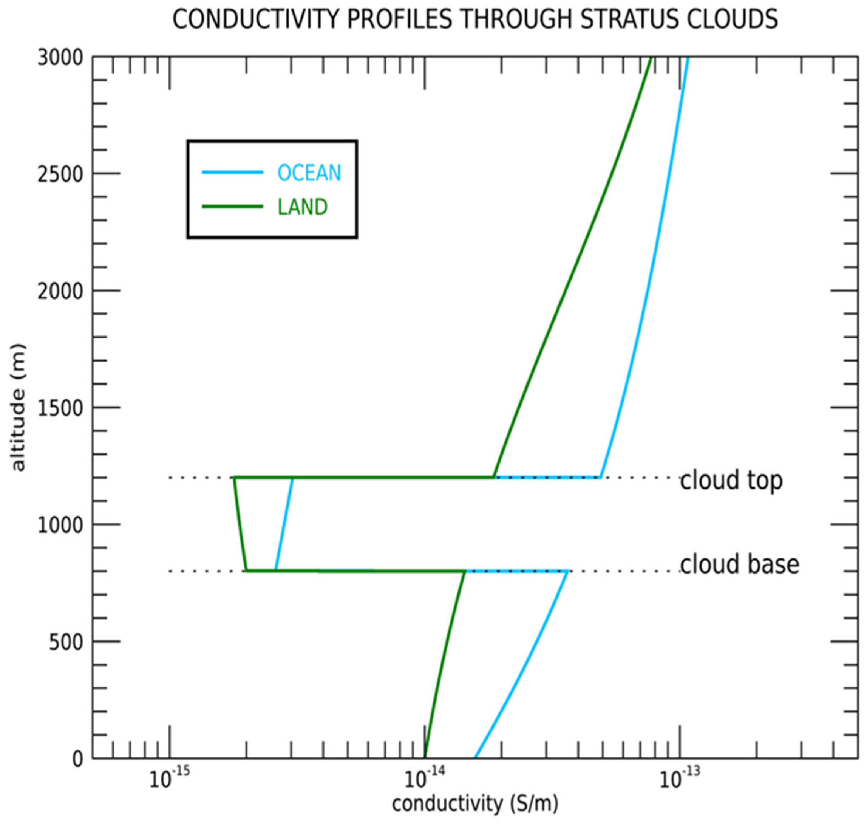
• A value of 1.6 × 10⁻¹⁴ S/m at mean sea level over the unpolluted ocean;
• A value of 1.0 × 10⁻¹⁴ S/m above the land surface, where the air is polluted so that the ions are larger, heavier, and hence less mobile than in pure air;
• The air conductivity inside the stratus cloud is less than that in the surrounding air at the same level by a factor ~10 for the same reason, the ions being scavenged by small water droplets; observations and a theoretical discussion which support these profiles have been presented by Harrison et al. [47].

Figure 3. The model air conductivity profiles through stratus clouds, at altitudes between 0.8 and 1.2 km, above the land (black line) or ocean (blue line), show that there is an order of magnitude reduction in the air conductivity inside the clouds compared with that in the surrounding air. From Rycroft et al. [10].

Figure 3. The model air conductivity profiles through stratus clouds, at altitudes between 0.8 and 1.2 km, above the land (black line) or ocean (blue line), show that there is an order of magnitude reduction in the air conductivity inside the clouds compared with that in the surrounding air. From Rycroft et al. [10].

In their Figure 5, Rycroft et al. [10] considered the mutual capacitance to Earth of such a stratus cloud layer. They found that this representation of the GEC gave a time constant of 8.3 min.

The eruption of the Icelandic volcano Grímsvötn during May 2011 produced substantial volcanic lightning (Figure 4a), which occurred in several periodic pulses (Figure 4b). Around midnight UT on 21 May 2011, when, globally, lightning is approaching its daily minimum, Figure 4c shows that the Grímsvötn eruption provided a major source (∼20%) of the global lightning flashes as determined by the UK Met Office lightning monitoring system.

At Reading, which had mostly undisturbed weather from 21 May 2011 into 22 May, measurements were made of the potential gradient (PG) and the downward current flowing to an isolated flat plate. In the PG data, a pulse is seen around the same time as the lightning pulse, suggesting an association between them (Figure 4d). Further, the air–Earth current showed a maximum at the same time, indicating that the PG pulse was associated with current flow changes (i.e., from the global circuit), rather than from local air conductivity changes. In addition, the magnitude of the PG variation is about 20%, comparable with the Grímsvötn lightning contribution to the total lightning count rate. After forming 1 min averages of the PG and Grímsvötn lightning flash rate, their correlation was calculated; the greatest correlations with the Grímsvötn lightning flash rate are found to be obtained with the PG at Reading about 8 to 14 min later, with a slight maximum at 9 min of lag. This is interpreted as being the time constant of the GEC. This time constant of 9 min was confirmed in an OrCAD PSpice model with an extra lightning source due to the volcano (Figure 8 of Rycroft et al. [10] and a semi-fair-weather PG situation.

Rycroft et al. [28] have discussed the concept of the global circuit capacitor and two new methods of deriving the time constant, τ, of the DC GEC. The first involves a more complex analogue electrical engineering model of the GEC, including low-level stratus clouds over ~30% of the Earth’s surface, the remaining 70% being cloudless. Note that the proportion of the Earth’s surface covered by thunderstorms or electrified shower clouds is negligibly small. The value of τ found was 10.2 min. The second method considered the dielectric and conducting properties of the atmosphere theoretically, the height at which ELF electromagnetic radiation is absorbed, and the importance of the dielectric relaxation time of the atmosphere just above the Earth’s surface, ε₀/σ₀, where σ₀ is the electrical conductivity of the surface air. The value of τ obtained was 7.6 min, in good accord with the experimental finding of Bor et al. [48] for volcanic lightning produced by the Hunga Tonga-Hunga Ha’apai eruption of January 2022.

7. Recent Observations of GEC Parameters

At the end of a review paper on the DC and AC GECs, Rycroft and Harrison [49] suggested that a continued search should be made for signatures in the vertical electric field observed near the Earth’s surface and throughout the atmosphere due to the following:

• Solar flares or coronal mass ejections;
• Forbush decreases;
• Solar proton events;
• Auroral activity; and
• Gigantic jets.

To this end, and amongst other objectives, networks of instruments to measure the near-surface electric field, E, using field mills, current density, J, and other parameters have been established around the world. Examples are a South American network (Tacza et al. [50,51]), two Polish stations (Michnowski et al. [52]), a set-up in Alaska (Lavigne et al. [53], Lavigne and Liu [54]), and the GloCAEM (Global Coordination of Atmospheric Electricity Measurements) project (Nicoll et al. [55]). Data from the GloCAEM station in the Negev Desert in Israel have been used by Yair and Yaniv [56] to study the effects of fog on E.

New instruments for measuring E have been reviewed by Povschenko and Bazhenov [57]. The availability of new field mills, particularly those that can operate successfully under all weather conditions (see Harrison and Marlton [58] and Section 2.3 of Harrison [39]), are the reason behind these recent experimental campaigns. The other important aspect is that there is now agreement on criteria for the definition of fair-weather conditions (Harrison and Nicoll [27]); this means that the effects of local meteorological conditions can be minimised, which enhances the possibility of GEC effects being detectable.

Büsken [59] published details of five field mills set-up at a high energy cosmic ray observatory to observe thunderstorm associated electric field changes (Wormell [12]) and possible effects due to terrestrial gamma ray flashes (TGFs, see Lyu et al. [60]). A network of 34 field mills has been established at the Kennedy Space Center (see https://ghrc.nsstc.nasa.gov/, accessed 16 March 2025) to investigate large electric fields in the vicinity of thunderstorms (Wormell [12]), which are a danger to space launch systems. Lucas et al. [61] used data from an array of field mills and from meteorological instruments there to study wind-borne space charges and the reduced conductivity (by a factor of 3) of air inside clouds compared with that outside.

I now give a few examples of recent research on these topics (a) to (e) and related ones. Riabova and Spivak [62] reported, during strong magnetic storms (which are usually associated with coronal mass ejection events on the Sun), marked surface electric field changes and J values up to 80 pA/m². Anisimov et al. [63] found increased values of E within ±4 h of a large magnetic storm, and Li et al. [64,65] reported similar variations. However, Figure 11 of Pilipenko et al. [66] shows that, during the large magnetic storm of 5 April 2010, the electric field between 09 and 10 UT was significantly reduced at four out of six stations where it was recorded, resembling the bay-like appearance of the horizontal magnetograms at all six, close by geomagnetic observatories at that time (see Figure 3 of Pilipenko et al. [66]). At relatively low latitudes, in Israel, Yaniv et al. [67] found that even strong geomagnetic storms did not produce any effects on E that were noticeable above the meteorological noise.

Tacza et al. [68] reported that the surface electric field at a high-altitude station in Argentina increased in association with a quite large (>7%) Forbush decrease. Tacza and Raulin [51] found that for large Forbush decreases, where the cosmic ray flux reduction was >10%, the surface electric field at this station exhibited a clear increase in the PG lasting for ~2 h; however, for small Forbush decreases, there was no such increase. In relation to Tacza et al. [69], Li et al. [64] stated that “there was no deviation in the atmospheric electric field values after solar flares, and the atmospheric electric field increased by approximately 10 V/m after solar proton events”. Concerning auroral activity, Table 2 of Michnowski et al. [52]) showed that at Hornsund, on Spitsbergen, in the Arctic, the PG at ground level is increased during substorms in the midnight and dawn sectors but decreased in the dusk sector. This broadly confirmed the results of Kleimenova et al. [70].

From Schumann resonance observations at two high latitude stations in the Arctic and Antarctic, Nickolaenko et al. [71] showed that the ELF radio wave reflection height in the lower ionosphere increased by ~1 km as solar activity declined from 2015 to 2018.

8. Can Pre-Seismic or Seismic Phenomena Affect the GEC?

Parrot et al. [72] reviewed the many observations made by different space-borne instruments associated with the precursors of major seismic events. These observations are of different ionospheric parameters and of thermal radiation from the surface of the Earth in the vicinity of large earthquakes. Chen et al. [73] have also reviewed this area of research. In the four days before earthquakes, Peddi Naidu et al. [74] reported the changed behaviour of the sporadic E-layer and F2-region of the ionosphere, and also the phase of 16 kHz radio signals propagating in the Earth–ionosphere waveguide from the UK to India, during seismically active periods. Boudjada et al. [75] reported similar phase changes before the large Turkey/Syria earthquake of 2023. Li et al. [76] have investigated possible precursor effects of a large earthquake in Mexico in September 2022.

Sorokin et al. [77] have analysed various theoretical models whereby pre-seismic or seismic phenomena may change a range of atmospheric and ionospheric parameters. They compare these with claimed observations of changes in the electric fields and currents in the atmosphere and ionosphere, and related changes in both ULF pulsations and ELF electromagnetic waves. As a best fit between experimental and theoretical considerations, they propose an electrodynamic model based on the perturbation of the conductivity current in the global atmosphere–ionosphere electric circuit due to the injection of charged aerosols into the atmosphere before and during an earthquake.

Denisenko and Bakhmetieva [78] discussed the suggestion of Harrison et al. [79,80] that, before a large earthquake, there could be a larger than usual emanation of radon from the fracturing ground that would enhance the conductivity of the air above ground level and hence reduce the resistance of the air column up to the ionosphere. The consequent electric field change in this column could change the height of the D-region. Denisenko and Bakhmetieva [78] showed theoretically that, in the D-region, the vertical electric field component over an area of intense radon emanation would double in comparison with the fair-weather field. They modelled the detailed spatial pattern of disturbances of electric fields and currents in the atmosphere and ionosphere over the region of enhanced radon emanation. They deduced that the doubled D-region vertical electric field E would be found in a region of ~50 km radius above the enhanced radon source.

With B the geomagnetic field strength, this could be expected to create an E ^ B/B² drift of the ionospheric plasma in this region in an eastward direction; this would be opposed by collisions with neutral gas atoms and molecules. The collisions between ions and neutrals predominantly decelerate the ions, rather than accelerate the neutrals. Figure 6 of Denisenko and Bakhmetieva [78]) shows that, at ~85 km altitude, the vertical component of E, E_z, is ~10⁻⁸ V/m, which, with a typical Northward component of B, B_x ~15,000 nT, gives a drift velocity v_y ~−6.10⁻⁵ m/s, which is negligibly small. With their Equation (4), Harrison et al. [79] estimated that the upward velocity of electrons, v_z, in the low ionosphere above the radon-emitting region where the electron density is ~10⁷ m⁻³, would be ~1 m/s, i.e., ~0.06 km/minute, or ~3.6 km/hour; such a velocity could be detectable experimentally. It would be interesting to explore, theoretically, whether changes associated with a doubled E_z in a localised part of the D-region might occur, e.g., via chemical mechanisms.

Pisa et al. [81] confirmed previously reported results of a very small, but statistically significant, decrease in naturally occurring VLF radio wave intensities observed by instruments aboard the DEMETER satellite in the topside ionosphere. The wave intensity decrease at a frequency of about 1.7 kHz is observed only during the night and only for shallow earthquakes. This can be explained by increases in the cut-off frequency of the Earth–ionosphere waveguide and so a lowering of the D-region ionosphere caused by imminent earthquakes. Pisa et al. [82] showed that the intensity decrease at ~1.7 kHz was ~2 dB, and that it occurred for a few hours before the main shocks. This could be explained by the Harrison et al. [79] mechanism.

Pulinets [83] and Pulinets and Herrera [84] have discussed earthquake precursors in relation to the following:

• Understanding the physical background of the earthquake precursors’ generation, some of which involve the GEC;
• Developing technologies for their reliable identification, and determining the main earthquake parameters, namely their time, place, and magnitude;
• Organising their real-time monitoring and developing short-term forecasts.

A recent paper by Surkov [85] comprehensively reviewed theoretical studies of the sub-audio, or ultra-low-frequency (ULF, <1 Hz), electromagnetic fields and currents in the lithosphere, atmosphere, and ionosphere, plus changes in the conductivity of these three media and of other non-seismic (e.g., thermal, Ouzounov et al. [86], Pulinets et al. [87] phenomena accompanying earthquakes or as precursors to earthquakes, both qualitatively and quantitatively. In relation to the GEC, Surkov [85] concludes that

• An earthquake of magnitude 7 on the Richter scale could generate a noisy ULF signal (up to ~1 nT or ~1 µV/m) that could be detectable above other ULF noise in the global electric circuit at a distance of only up to 100 or perhaps 300 km from the epicentre of the earthquake (his Section 2.2);
• There is no direct experimental evidence for the mobile positive hole (p-hole) theory of current carriers responsible for the rock conductivity in stressed rocks presented by Freund et al. [88]; because of contradictions with the values of three different realistic parameters, this theory presents unrealistic estimates of the magnitude of the earthquake precursor signals which are present in the GEC (his Section 2.3);
• The increased conductivity of air at up to ~1 km above the surface following the enhanced emission of radon from the Earth associated with seismic activity (Harrison et al. [79], Pulinets et al. [89]) decreases the total resistance of the column of air up to the ionosphere by ~20%; this would locally increase the current up to the ionosphere, which would increase the fair-weather current in the GEC (his Section 5.1);
• Any aerosol ions present will reduce the conductivity, which, in the presence of light winds (up to ~2 m/s) under fair-weather conditions, could cause large changes in the PG, up to 400 V/m, and for ~2 h, as has been observed before earthquakes (Smirnov [90]) (his Section 5.2);
• The possible coupling between infrared radiation anomalies and earthquakes (Pulinets and Ouzounov [91]) is “implausible” because quantitative estimates of the signals present in the GEC arising from these models are unrealistic and do not agree with observations (his Section 5.3);
• There is no theoretical explanation for how the claimed changes (e.g., Galvan et al. [92], Sunardi et al. [93], Li et al. [76]) to the total electron content of a column of ionospheric ionisation (in TEC units, 10¹⁶ m⁻²) before an earthquake could occur, although they might be caused by upward-propagating acoustic gravity waves in the atmosphere which could change the ionosphere and also the GEC (his Section 6);
• The increased current up to the ionosphere discussed in (3 above would increase the E-region density at night by ~0.004% and by day by an even smaller amount; such a small increase would not be detectable experimentally, so this aspect of the mechanism is “hardly plausible” (his Section 6.3);
• Because the timescale of discharging in natural ionisation levels by attachment is of the order of minutes at most, an enhanced emission of charged aerosols (rather than radon) from the ground before an earthquake (Sorokin and Novikov [94]) produces “only very weak ionospheric currents”, making models for this mechanism “seem questionable” (his Section 6.4).

It goes without saying that if there is a real earthquake precursor effect on the F-region of the ionosphere and on its TEC, the “signal” which causes that has to go through the D- and E-regions; a manifestation of that signal should appear there before the effect higher up. However, what that manifestation would be for very-long-wavelength acoustic waves remains unclear.

9. The DC and AC GECs and Human Health

The Scientific Committee on Emerging and Newly Identified Health Risks (SCENIHR) of the European Commission comprehensively reviewed the potential human health effects of the exposure to electromagnetic fields from ~1 Hz up to ~100 MHz (SCENIHR [95]). The report concentrated on possible effects due to radiation produced by electrical grid systems, laptop computers, and smart phones, rather than natural electromagnetic fields occurring in the DC GEC. Health risks associated with ELF radiation have been considered in Chapter 12 (pages 349–356) of a World Health Organisation report (WHO [96]).

Palmer et al. [97] reviewed research on the effect of variations in geomagnetic activity on human cardiovascular health. Possible mechanisms by which space weather, i.e., variations in solar and geophysical parameters, could affect human health were discussed and the most likely candidates investigated. The direct effects of natural extremely-low-frequency electric and magnetic fields appear implausible; a mechanism involving some form of resonant absorption (Cherry [98]) is more likely. The idea that the Schumann resonance signals in the AC GEC could be the global environmental signal absorbed by the human body, via a melatonin mechanism (see the review by Jammoul and Lawand [99]), thereby linking geomagnetic activity and human health was investigated. Price et al. [100] presented evidence for the link between electromagnetic fields in the Schumann resonance frequency range and those found in many living organisms, including humans. It is noteworthy that the dominant electrical activity of the human brain, which occurs over the visual-association part of the brain, are the so-called alpha waves (Brazier [101], Hima et al. [102]); these peak at between 8 and 13 Hz, i.e., close to the fundamental and second harmonic frequencies of the Schumann resonances.

Martel et al. [103] surveyed research that suggests that the circadian rhythm, which controls several physiological functions in the human body, can be influenced by light but also by Schumann resonances and changes in the GEC and the geomagnetic field, possibly by disrupting the circadian rhythm and downstream physiological functions. In a wide-ranging study, Martel et al. [104] described a series of observations indicating that light exposure, lifestyle habits, and electromagnetic fields regulate and influence biological rhythms in humans. Humans are sensitive to even small variations in light, temperature, and electromagnetic fields in the environment. It might not be entirely surprising that artificial light, solar storms, and sunspots can affect a wide range of human diseases and symptoms. Thus, the circadian rhythm, sunlight, and natural and anthropogenic electromagnetic fields may have a larger effect on human health than is usually considered. An extensive review of the interaction between Schumann resonance signals and the human body, particularly the nervous system, has recently been published by Nevoit et al. [105].

Mavromichalaki et al. [106] have presented several statistical studies of the effects of solar, geomagnetic, and cosmic ray activity on human physiological parameters, such as heart rate and blood pressure. Very recently, Cui et al. [107] reported statistically significant beneficial effects of bursts of 20 Hz magnetic fields generated by coils adjacent to the heads of patients with treatment-resistant depression. Rycroft et al. [28] have mentioned some GEC effects on spiders and bees, as well as on humans.

10. Conclusions

The subjects of both the DC and AC global electric circuits are alive and well in 2025—more research remains to be performed. The main conclusions drawn from this study are as follows:

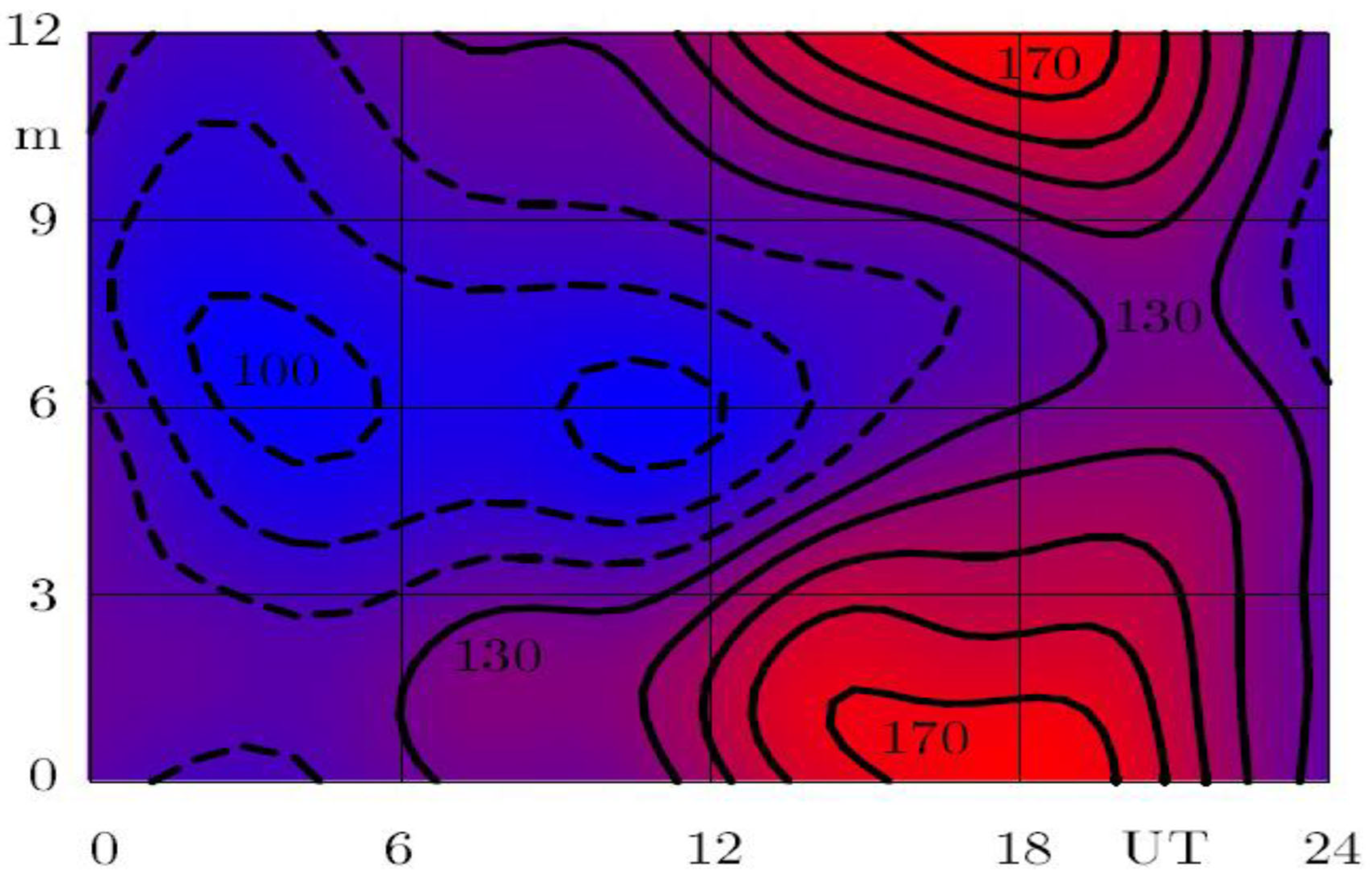
• The current I in the DC GEC of ~1 kA is generated by thunderstorms and electrified shower clouds; this maintains the ionospheric potential V at ~250 kV with respect to the Earth’s surface. The current flowing down through the fair-weather and semi-fair-weather atmosphere has a density J ~2 pA/m², and the resistance of the atmosphere, R, is ~250 Ω. The electric field E (or potential gradient, with the opposite sign) above the surface of the Earth varies from ~100 V/m at 04 UT during July to ~170 V/m at 18 UT in January; the UT variation on a particular day is called the Carnegie curve (Section 1 and Section 2).
• The positive charge density in the atmosphere near the Earth’s surface associated with the operation of the DC GEC and the consequent charge Q of −6 × 10⁵ C on the Earth (Wilson [3]) is only 0.3 pC/m³; this is smaller than typical values of the measured charge density that range from ~−20 to + 20 pC/m³. It is therefore impossible to gain information about the GEC, other than for its existence, from such observations (Section 3).
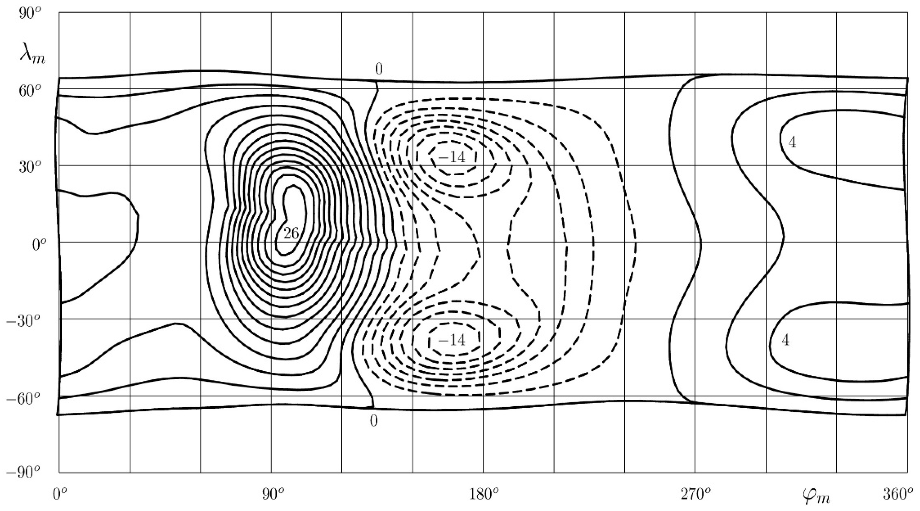
• A comprehensive theoretical model of the DC GEC has been published by Denisenko et al. [38]); using it, thunderstorm-generated electric fields can be estimated in the ionosphere. These cause low-latitude electrojets to flow in the ionosphere, which produce geomagnetic perturbations ~0.1 nT; they are too small to be detectable in the presence of those generate by ionospheric-wind-driven dynamo currents (Section 4).
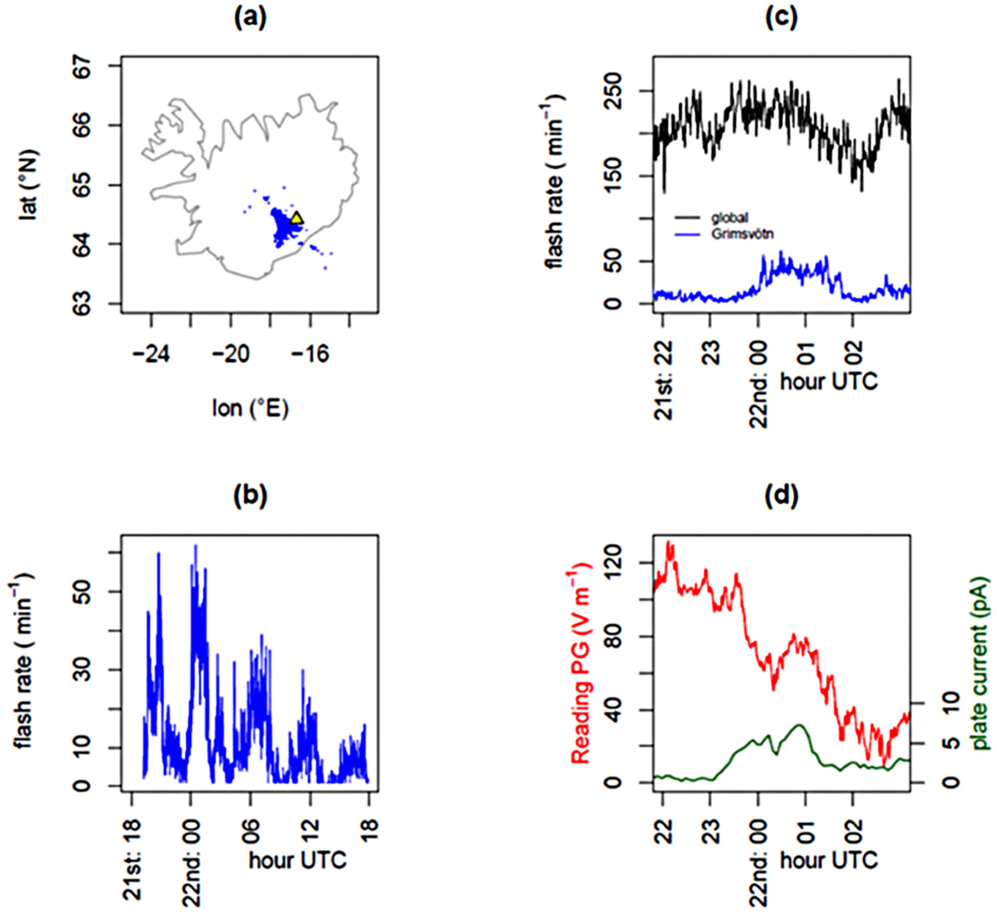
• With the capacitance C of the GEC being ~1.5 F, its CR time constant, τ, is modelled to be ~8 min. With a more complex model involving status clouds over 30% of the Earth, this value of τ is confirmed. More recent modelling studies by Rycroft et al. [28] have put τ at 10 min. The time constant derived experimentally from observations of the sudden excitation of the GEC by volcanic lightning is found to lie between 7 and 12 min (Section 5).
• It is unlikely that seismic activity, or earthquake precursors, can produce large enough electric fields in the ionosphere to cause detectable effects there, either by enhanced radon emission or by enhanced thermal emission from the earthquake region (Section 6).
• There is some evidence that, via a melatonin mechanism, Schumann resonance signals and alpha waves in the human brain may somehow be linked (Section 7).
• The GEC has the potential to act as a framework to study global climate change (Mironova et al. [108], Siingh et al. [22]) through its interactions with atmospheric processes on various scales.

References

1. Wilson, C.T.R. On the measurement of earth-air current and on the origin of atmospheric electricity. Proc. Camb. Phil. Soc. 1906, 13, 363–382. [Google Scholar]
2. Wilson, C.T.R. On the Measurement of the Atmospheric Electric Potential Gradient and the Earth-air Current. Proc. R. Soc. Lond. A 1908, 80, 537–547. [Google Scholar] [CrossRef]
3. Wilson, C.T.R. Investigations on lightning discharges and on the electric field of thunderstorms, Philos. Trans. R. Soc. Lond. A 1921, 221, 73–115. [Google Scholar] [CrossRef]
4. Wilson, C.T.R. Some thundercloud problems. J. Franklin Inst. 1929, 208, 1–12. [Google Scholar] [CrossRef]
5. Rycroft, M.J.; Israelsson, S.; Price, C. The global atmospheric electric circuit, solar activity and climate change. J. Atmos. Sol-Terr. Phys. 2000, 62, 1563–1576. [Google Scholar] [CrossRef]
6. Williams, E.R. The global electrical circuit: A review. Atmos. Res. 2009, 91, 140–152. [Google Scholar] [CrossRef]
7. Williams, E.R. Electricity in the Atmosphere: Global Electrical Circuit. Ref. Collect. Earth Syst. Environ. Sci. 2024, 13. [Google Scholar] [CrossRef]
8. Harrison, R.G. The cloud chamber and CTR Wilson’s legacy to atmospheric science. Weather 2011, 66, 276–279. [Google Scholar] [CrossRef]
9. Harrison, R.G. Fair Weather Atmospheric Electricity. J. Phys. Conf. Ser. 2011, 301, 012001. [Google Scholar] [CrossRef]
10. Rycroft, M.J.; Odzimek, A.; Harrison, R.G. Determining the time constant of the global atmospheric electric circuit through modelling and observations. J. Atmos. Sol.-Terr. Phys. 2024, 260, 106267. [Google Scholar] [CrossRef]
11. Wormell, T.W. Vertical electric currents below thunderstorms and showers. Proc. R. Soc. Lond. A. 1930, 127, 567–590. [Google Scholar] [CrossRef]
12. Wormell, T.W. Atmospheric electricity; some recent trends and problems. Q. J. R. Met. Soc. 1953, 79, 3–38. [Google Scholar] [CrossRef]
13. Wormell, T.W. Obituary. Q. J. R. Met. Soc. 1985, 111, 675. [Google Scholar] [CrossRef]
14. Aplin, K.L.; Harrison, R.G.; Füllekrug, M.; Lanchester, B.; Becker, F. A scientific career launched at the start of the space age: Michael Rycroft at 80. Hist. Geo Space Sci. 2020, 11, 105–121. [Google Scholar] [CrossRef]
15. Schumann, W.O. Über die strahlungslosen Eigenschwingungen einer leitenden Kugel, die von einer Luftschicht und einer Ionosphärenhülle umgeben ist. Z. Für Naturforschung. 1952, 7A, 149–154. [Google Scholar] [CrossRef]
16. Balser, M.; Wagner, C.A. Observations of Earth–Ionosphere Cavity Resonances. Nature 1960, 188, 638–641. [Google Scholar]
17. Rycroft, M.J. Resonances of the Earth-Ionosphere Cavity Observed at Cambridge, England. Radio Sci. J. Res. NBS 1965, 69D, 1071–1081. [Google Scholar]
18. Barr, R.; Llanwyn Jones, D.; Rodger, C.J. ELF and VLF Radio Waves. J. Atmos. Sol.-Terr. Phys. 2000, 62, 1689–1718. [Google Scholar]
19. Nickolaenko, A.P.; Hayakawa, M. Resonances in the Earth-Ionosphere Cavity; Springer: Berlin/Heidelberg, Germany, 2002; 380p, ISBN 9781402007545. [Google Scholar]
20. Nickolaenko, A.; Hayakawa, M. Schumann Resonance for Tyros: Essentials of Global Electromagnetic Resonance in the Earth–Ionosphere Cavity; Springer: Berlin/Heidelberg, Germany, 2014; 348p. [Google Scholar] [CrossRef]
21. Liu, J.; Huang, J.; Li, Z.; Zhao, Z.; Zeren, Z.; Shen, X.; Wang, Q. Recent Advances and Challenges in Schumann Resonance Observations and Research. Remote Sens. 2023, 15, 3557. [Google Scholar] [CrossRef]
22. Siingh, D.; Singh, R.P.; Jeni Victor, N.; Kamra, A.K. The DC and AC global electric circuits and climate. Earth-Sci. Rev. 2023, 244, 104542. [Google Scholar] [CrossRef]
23. Mülheisen, R. The global circuit and its parameters. In Electrical Processes in Atmospheres; Dolezalek, H., Reiter, R., Eds.; Steinkopf Verlag: Heidelberg, Germany, 1977; pp. 467–476. [Google Scholar]
24. Harrison, R.G. The global atmospheric electrical circuit and climate. Surv. Geophys. 2004, 25, 441–484. [Google Scholar] [CrossRef]
25. Harrison, R.G. The Carnegie curve. Surv. Geophys. 2013, 34, 209–232. [Google Scholar] [CrossRef]
26. Harrison, R.G. Behind the curve: A comparison of historical sources for the Carnegie curve of the global atmospheric electric circuit. Hist. Geo Space Sci. 2020, 11, 207–213. [Google Scholar] [CrossRef]
27. Harrison, R.G.; Nicoll, K.A. Fair weather criteria for atmospheric electricity measurements. J. Atmos. Sol.-Terr. Phys. 2018, 179, 239–250. [Google Scholar] [CrossRef]
28. Rycroft, M.J.; Nickolaenko, A.P.; Harrison, R.G.; Odzimek, A. The global circuit capacitor and two new ways of deriving the time constant of the global atmospheric electric circuit. J. Atmos. Sol.-Terr. Phys. 2025; submitted. [Google Scholar]
29. Aplin, K.L. Instrumentation for Atmospheric Ion Measurements. Ph.D. Thesis, University of Reading, Reading, UK, 2000; 274p. [Google Scholar]
30. Aplin, K.L.; Harrison, R.G.; Rycroft, M.J. Investigating Earth’s atmospheric electricity: A role model for planetary studies. Space Sci. Rev. 2008, 137, 11–27. [Google Scholar] [CrossRef]
31. Anisimov, S.V.; Galichenko, S.V.; Aphinogenov, K.V.; Klimanova, E.V.; Kozmina, A.S. Small air ion statistics near the earth’s surface. Atmos. Res. 2022, 267, 105193. [Google Scholar]
32. Nicoll, K.A.; Harrison, R.G. Experimental determination of layer cloud edge charging from cosmic ray ionisation. Geophys. Res. Lett. 2010, 37, L13802. [Google Scholar] [CrossRef]
33. Nicoll, K.A.; Harrison, R.G. Charge measurements in stratiform cloud from a balloon based sensor. J. Phys. Conf. Ser. 2011, 301, 012003. [Google Scholar] [CrossRef]
34. Nicoll, K.A.; Harrison, R.G. Stratiform cloud electrification: Comparison of theory with multiple in-cloud measurements. Q. J. R. Met. Soc. 2016, 142, 2679–2691. [Google Scholar] [CrossRef]
35. Anisimov, S.V.; Galichenko, S.V.; Aphinogenov, K.V.; Klimanova, E.V.; Prokhorchuk, A.A.; Kozmina, A.S.; Guriev, A.V. Mid-latitude atmospheric boundary layer electricity: A study by using a tethered balloon platform. Atmos. Res. 2021, 250, 105355. [Google Scholar] [CrossRef]
36. Hirsikko, A.; Nieminen, T.; Gagn’e, S.; Lehtipalo, K.; Manninen, H.E.; Ehn, M.; Hõrrak, U.; Kerminen, V.-M.; Laakso, L.; McMurry, P.H.; et al. Atmospheric ions and nucleation: A review of observations. Atmos. Phys. Chem. 2011, 11, 767–798. [Google Scholar] [CrossRef]
37. Tinsley, B.A. The influence of the solar wind electric and magnetic fields on the latitude and temporal variations of the current density, Jz, of the global electric circuit, with relevance to weather and climate. J. Atmos. Sol.-Terr. Phys. 2024, 265, 106355. [Google Scholar] [CrossRef]
38. Denisenko, V.V.; Rycroft, M.J.; Harrison, R.G. Mathematical Simulation of the Ionospheric Electric Field as a Part of the Global Electric Circuit. Surv. Geophys. 2019, 40, 1–35, Erratum in Surv. Geophys. 2019, 40, 37. [Google Scholar] [CrossRef]
39. Harrison, R.G. Measuring electrical properties of the lower troposphere using enhanced meteorological radiosondes. Geosci. Instrum. Method Data Syst. 2022, 11, 37–57. [Google Scholar] [CrossRef]
40. Khegai, V.V.; Korsunova, L.P.; Legen’ka, A.D. Estimation of a Tropospheric Electric Field Associated with the African Zone of Thunderstorm Activity that Penetrates the Ionosphere. Geomagn. Aeron. 2021, 61, 559–564. [Google Scholar] [CrossRef]
41. Liu, X.; Li, L.; Zhang, Y.; Xue, H. Ionospheric currents and nightside ionospheric magnetic fields calculated by TIE-GCM (in Chinese). Chin. J. Space Sci. 2018, 38, 29–36. [Google Scholar] [CrossRef]
42. Denisenko, V.V.; Rycroft, M.J. The ionospheric equatorial electrojets generated by low latitude thunderstorms. J. Atmos. Sol.-Terr. Phys. 2021, 221, 105704. [Google Scholar] [CrossRef]
43. Denisenko, V.V.; Rycroft, M.J. WWLLN data used to model the ionospheric electric field generated by thunderstorms. Ann. Geophys. 2022, 65, PA536. [Google Scholar] [CrossRef]
44. Denisenko, V.V.; Rycroft, M.J. Seasonal dependence of the equatorial electrojets generated by thunderstorms. Adv. Space Res. 2023, 73, 3464–3471. [Google Scholar] [CrossRef]
45. Holzworth, R.H.; Bering, E.A., III; Kokorowski, M.F.; Lay, E.H.; Reddell, B.; Kadokura, A.; Yamagishi, H.; Sato, N.; Ejiri, M.; Hirosawa, H.; et al. Balloon observations of temporal variation in the global circuit compared to global lightning activity. Adv. Space Res. 2005, 36, 2223–2228. [Google Scholar] [CrossRef]
46. Haldoupis, C.; Rycroft, M.; Williams, E.; Price, C. Is the “Earth-ionosphere capacitor” a valid component in the atmospheric global electric circuit? J. Atmos. Sol.-Terr. Phys. 2017, 164, 127–131. [Google Scholar] [CrossRef]
47. Harrison, R.G.; Nicoll, K.A.; Mareev, E.; Slyunyaev, N.; Rycroft, M.J. Extensive layer clouds in the global electric circuit: Their effects on vertical charge distribution and storage. Proc. R. Soc. A 2020, 476, 20190758. [Google Scholar] [CrossRef] [PubMed]
48. Bór, J.; Bozóki, T.; Sátori, G.; Williams, E.; Behnke, S.A.; Rycroft, M.J.; Buzás, A.; Silva, H.G.; Kubicki, M.; Said, R.; et al. Responses of the AC/DC Global Electric Circuit to Volcanic Electrical Activity in the Hunga Tonga-Hunga Ha’apai Eruption on 15 January 2022. J. Geophys. Res. Atmos. 2023, 128, e2022JD038238. [Google Scholar] [CrossRef]
49. Rycroft, M.J.; Harrison, R.G. Electromagnetic atmosphere-plasma coupling: The global electric circuit. Space Sci. Rev. 2012, 168, 363–384. [Google Scholar] [CrossRef]
50. Tacza, J.; Raulin, J.-P.; Macotela, E.; Norabuena, E.; Fernandez, G.; Correia, E.; Rycroft, M.J.; Harrison, R.G. A new South American network to study the atmospheric electric field and its variations related to geophysical phenomena. J. Atmos. Sol.-Terr. Phys. 2014, 120, 70–79. [Google Scholar] [CrossRef]
51. Tacza, J.; Li, G.; Raulin, J.-P. Effects of Forbush Decreases on the global electric circuit. Space Weather 2024, 22, e2023SW003852. [Google Scholar] [CrossRef]
52. Michnowski, S.; Odzimek, A.; Kleimenova, N.G.; Kozyreva, O.V.; Kubicki, M.; Klos, Z.; Israelsson, S.; Nikiforova, N.N. Review of Relationships Between Solar Wind and Ground-Level Atmospheric Electricity: Case Studies from Hornsund, Spitsbergen, and Swider, Poland. Surv. Geophys. 2021, 42, 757–801. [Google Scholar] [CrossRef]
53. Lavigne, T.; Liu, C.; Hill, J.; Bruning, E. Observations from the one year electric field Study-North Slope of Alaska (OYES-NSA) field campaign, and their implications for observing the distribution of global electrified cloud activity. J. Atmos. Sol.-Terr. Phys. 2021, 214, 105528. [Google Scholar] [CrossRef]
54. Lavigne, T.; Liu, C. Relationships among diurnal variations of polar night cloud, precipitation, surface temperatures, and the fair-weather return current of the global electric circuit (GEC). J. Atmos. Sol.-Terr. Phys. 2023, 244, 106026. [Google Scholar] [CrossRef]
55. Nicoll, K.A.; Harrison, R.G.; Barta, V.; Bor, J.; Brugge, R.; Chillingarian, A.; Chum, J.; Georgoulias, A.K.; Guha, A.; Kourtidis, K.; et al. A global atmospheric electricity monitoring network for climate and geophysical research. J. Atmos. Sol.-Terr. Phys. 2019, 184, 18–29. [Google Scholar] [CrossRef]
56. Yair, Y.; Yaniv, R. The Effects of Fog on the Atmospheric Electrical Field Close to the Surface. Atmosphere 2023, 14, 549. [Google Scholar] [CrossRef]
57. Povschenko, O.; Bazhenov, V. Analysis of Modern Atmospheric Electrostatic Field Measuring Instruments and Methods. Technol. Audit. Prod. Reserves 2023, 4, 16–24. [Google Scholar] [CrossRef]
58. Harrison, R.G.; Marlton, G.J. Fair weather electric field meter for atmospheric science platforms. J. Electrostat. 2020, 107, 103489. [Google Scholar] [CrossRef]
59. Büsken, M.; for the Pierre Auger Collaboration. A new network of electric field mills at the Pierre Auger Observatory. J. Phys. Conf. Ser. 2022, 2398, 012004. [Google Scholar] [CrossRef]
60. Lyu, F.; Zhang, Y.; Lu, G.; Zhu, B.; Zhang, H.; Xu, W.; Xiong, S.; Lyu, W. Recent observations and research progresses of terrestrial gamma-ray flashes during thunderstorms. Sci. China Earth Sci. 2023, 66, 435–455. [Google Scholar] [CrossRef]
61. Lucas, G.M.; Thayer, J.P.; Deierling, W. Statistical analysis of spatial and temporal variations in atmospheric electric fields from a regional array of field mills. J. Geophys. Res. Atmos. 2017, 122, 1158–1174. [Google Scholar] [CrossRef]
62. Riabova, S.A.; Spivak, A.A. Variations of Electrical Characteristics of the Surface Atmosphere during Magnetic Storms. Dokl. Earth Sci. 2021, 497, 246–251. [Google Scholar] [CrossRef]
63. Anisimov, S.V.; Shikhova, N.M.; Kleimenova, N.G. Response of a Magnetospheric Storm in the Atmospheric Electric Field of the Midlatitudes. Geomagn. Aeron. 2021, 61, 180–190. [Google Scholar] [CrossRef]
64. Li, L.; Chen, T.; Shen, C.; Ti, S.; Wang, S.; Cai, C.; Li, W.; Luo, J. Near-surface atmospheric electric field changes through magnetic clouds via coronal mass ejections. Geosci. Lett. 2023, 10, 45. [Google Scholar] [CrossRef]
65. Li, W.; Sun, Z.; Chen, T.; Yan, Z.; Luo, J.; Xu, Q.; Ma, Z. Different Effects of a Super Storm on Atmospheric Electric Fields at Different Latitudes. Atmosphere 2024, 15, 1314. [Google Scholar] [CrossRef]
66. Pilipenko, V.; Smirnov, S.E.; Frank-Kamenetsky, A.V.; Martinez-Bedenko, V.A. An electrical storm during a magnetic storm on April 5, 2010. Izv. Atmos. Ocean. Phys. 2024, 60, 1555-628X. Available online: https://link.springer.com/journal/volumesAndIssues/11485 (accessed on 10 March 2025).
67. Yaniv, R.; Yair, Y.; Price, C.; Reuveni, Y. No Response of Surface-Level Atmospheric Electrical Parameters in Israel to Severe Space Weather Events. Atmosphere 2023, 14, 1649. [Google Scholar] [CrossRef]
68. Tacza, J.; Odzimek, A.; Tueros Cuadros, E.; Raulin, J.-P.; Kubicki, M.; Fernandez, G.; Marun, A. Investigating effects of solar proton events and Forbush decreases on ground-level potential gradient recorded at middle and low latitudes and different altitudes. Space Weather 2022, 20, e2021SW002944. [Google Scholar] [CrossRef]
69. Tacza, J.; Raulin, J.-P.; Mendonca, R.R.S.; Makhmutov, V.S.; Marun, A.; Fernandez, G. Solar effects on the atmospheric electric field during 2010–2015 at low latitudes. J. Geophys. Res. Atmos. 2018, 123, 11970–11979. [Google Scholar] [CrossRef]
70. Kleimenova, N.; Kozyrova, O.; Michnowski, S.; Kubicki, M. Influence of geomagnetic disturbances on atmospheric electric field (Ez) variations at high and middle latitudes. J. Atmos. Sol.-Terr. Phys. 2013, 99, 117–122. [Google Scholar] [CrossRef]
71. Nickolaenko, A.P.; Hayakawa, M.; Koloskov, O. Schumann resonance as a remote sensor of lower ionosphere and global thunderstorms as based on the long-term observations at Antarctic and Arctic stations. J. Atmos. Sol.-Terr. Phys. 2025, 269, 106465. [Google Scholar] [CrossRef]
72. Parrot, M.; Tramutoli, V.; Liu, T.J.Y.; Pulinets, S.; Ouzounov, D.; Genzano, N.; Lisi, M.; Hattori, K.; Namgaladze, A. Atmospheric and ionospheric coupling phenomena associated with large earthquakes. Eur. Phys. J. Spec. Top. 2021, 230, 197–225. [Google Scholar] [CrossRef]
73. Chen, H.; Han, P.; Hattori, K. Recent Advances and Challenges in the Seismo-Electromagnetic Study: A Brief Review. Remote Sens. 2022, 14, 5893. [Google Scholar] [CrossRef]
74. Peddi Naidu, P.; Madhavi Latha, T.; Madhusudhana Rao, D.N.; Indira Devi, M. Anomalous behavior of the ionosphere before strong earthquakes. Indian J. Phys. 2017, 91, 1467–1476. [Google Scholar] [CrossRef]
75. Boudjada, M.Y.; Biagi, P.F.; Eichelberger, H.U.; Nico, G.; Schwingenschuh, K.; Galopeau, P.H.M.; Solovieva, M.; Contadakis, M.; Denisenko, V.; Lammer, H.; et al. Unusual Sunrise and SunsetTerminator Variations in the Behavior of Sub-Ionospheric VLF Phase and Amplitude Signals Prior to the Mw7.8 Turkey Syria Earthquake of 6 February 2023. Remote Sens. 2024, 16, 4448. [Google Scholar] [CrossRef]
76. Li, Z.; Tao, Z.; Zhang, J.; Cao, Y. Analysis of Seismo-ionospheric Anomaly Disturbance Associated with the Mw7.6 Mexico Earthquake on 19 September 2022. Res. Sq. 2025; submitted. [Google Scholar] [CrossRef]
77. Sorokin, V.M.; Chmyrev, V.M.; Hayakawa, M. A Review on Electrodynamic Influence of Atmospheric Processes to the Ionosphere. Open J. Earthq. Res. 2020, 9, 113–141. [Google Scholar] [CrossRef]
78. Denisenko, V.V.; Bakhmetieva, N.V. Disturbance of the Electric Field in the D-Region of the Ionosphere with an Increase in Radon Emanation. Geomagn. Aeron. 2024, 64, 673–681. [Google Scholar] [CrossRef]
79. Harrison, R.G.; Aplin, K.L.; Rycroft, M.J. Atmospheric electricity coupling between earthquake regions and the ionosphere. J. Atmos. Sol.-Terr. Phys. 2010, 72, 376–381. [Google Scholar] [CrossRef]
80. Harrison, R.G.; Aplin, K.L.; Rycroft, M.J. Brief Communication: Earthquake–cloud coupling through the global atmospheric electric circuit. Nat. Hazards Earth Syst. Sci. 2014, 14, 773–777. [Google Scholar] [CrossRef]
81. Píša, D.; Parrot, M.; Santolík, O. Ionospheric density variations recorded before the 2010 Mw 8.8 earthquake in Chile. J. Geophys. Res. 2011, 116, A08309. [Google Scholar] [CrossRef]
82. Píša, D.; Nemec, F.; Santolík, O.; Parrot, M.; Rycroft, M. Additional attenuation of natural VLF electromagnetic waves observed by the DEMETER spacecraft resulting from preseismic activity. J. Geophys. Res. Space Phys. 2013, 118, 5286–5295. [Google Scholar] [CrossRef]
83. Pulinets, S.A. Physical bases of the short-term forecast of earthquakes. Astron. Astrophys. Trans. (AApTr) 2023, 34, 65–84. [Google Scholar] [CrossRef]
84. Pulinets, S.; Herrera, V.M.V. Earthquake Precursors: The Physics, Identification, and Application. Geosciences 2024, 14, 209. [Google Scholar] [CrossRef]
85. Surkov, V.V. An Overview of Theoretical Studies of Non-Seismic Phenomena Accompanying Earthquakes. Surv. Geophys. 2025, 46, 7–70. [Google Scholar] [CrossRef]
86. Ouzounov, D.; Pulinets, S.; Hattori, K.; Taylor, P. (Eds.) Pre-Earthquake Processes; a Multidisciplinary Approach to Earthquake Prediction Studies; AGU/Wiley: Washington, DC, USA, 2018; 365p. [Google Scholar] [CrossRef]
87. Pulinets, S.; Ouzounov, D.; Karelin, A.; Boyarchuk, K. Earthquake Precursors in the Atmosphere and Ionosphere: New Concepts; Springer: Dordrecht, The Netherlands, 2023; 314p. [Google Scholar] [CrossRef]
88. Freund, F.; Ouillon, G.; Scoville, J.; Sornette, D. Earthquake precursors in the light of peroxy defects theory: Critical review of systematic observations. Eur. Phys. J. Spec. Top. 2021, 230, 7–46. [Google Scholar] [CrossRef]
89. Pulinets, S.; Mironova, I.; Miklyaev, P.; Petrova, T.; Shitov, A.; Karagodin, A. Radon Variability as a Result of Interaction with the Environment. Atmosphere 2024, 15, 167. [Google Scholar] [CrossRef]
90. Smirnov, S. Negative anomalies of the Earth’s electric field as earthquake precursors. Geosciences 2020, 10, 10. [Google Scholar] [CrossRef]
91. Pulinets, S.; Ouzounov, D. Lithosphere-Atmosphere-Ionosphere Coupling (LAIC) model—A unified concept for earthquake precursors validation. J. Asian Earth Sci. 2011, 41, 371–382. [Google Scholar]
92. Galvan, D.A.; Komjathy, A.; Hickey, M.P.; Stephens, P.; Snively, J.; Song, Y.T.; Butala, M.D.; Mannucci, A.J. Ionospheric signatures of Tohoku-Oki tsunami of March 11, 2011: Model comparisons near the epicenter. Radio Sci. 2012, 47, RS4003. [Google Scholar] [CrossRef]
93. Sunardi, B.; Muslim, B.; Sakya, A.E.; Rohadi, S.; Sulastri, S.; Murjaya, J. Ionospheric earthquake effects detection based on Total Electron Content (TEC) GPS correlation. IOP Conf. Ser. Earth Environ. Sci. 2018, 132, 012014. [Google Scholar] [CrossRef]
94. Sorokin, V.M.; Novikov, V.A. A model of TEC perturbations possibly related to seismic activity. Ann. Geoph. 2023, 66, 642. [Google Scholar] [CrossRef]
95. SCENIHR. Health Effects of Electromagnetic Fields; European Commission: Brussels, Belgium, 2015; 288p, ISBN 978-92-79-30134-6. [Google Scholar]
96. WHO. Environmental Health Criteria 238, Extremely Low Frequency Fields; WHO: Geneva, Switzerland, 2007; 510p, ISBN 978-92-4-157238-5. [Google Scholar]
97. Palmer, S.J.; Rycroft, M.J.; Cermack, M. Solar and geomagnetic activity, extremely low frequency magnetic and electric fields and human health at the Earth’s surface. Surv. Geophys. 2006, 27, 537–595. [Google Scholar] [CrossRef]
98. Cherry, N. Schumann Resonances, a plausible biophysical mechanism for the human health effects of solar/geomagnetic activity. Nat. Hazards 2002, 26, 279–331. [Google Scholar] [CrossRef]
99. Jammoul, M.; Lawand, N. Melatonin: A Potential Shield against Electromagnetic Waves. Curr. Neuropharmacol. 2022, 20, 648–660. [Google Scholar] [CrossRef]
100. Price, C.; Williams, E.; Elhalel, G.; Sentman, D. Natural ELF fields in the atmosphere and in living organisms. Int. J. Biometeorol. 2021, 65, 85–92. [Google Scholar] [CrossRef]
101. Brazier, M.A. The analysis of brain waves. Sci. Am. 1962, 206, 152–153. [Google Scholar] [PubMed]
102. Hima, C.S.; Asheeta, A.; Nair, C.C.; Nair, S.M.J. A review on brainwave therapy. World J. Pharm. Sci. 2020, 8, 59–66. [Google Scholar]
103. Martel, J.; Chang, S.-H.; Chevalier, G.; Ojcius, D.M.; Young, J.D. Influence of electromagnetic fields on the circadian rhythm: Implications for human health and disease. Biomed. J. 2023, 46, 48–59. [Google Scholar] [CrossRef] [PubMed]
104. Martel, J.; Rouleau, N.; Murugan, N.J.; Chin, W.-C.; Ojcius, D.M.; Young, J.D. Effects of light, electromagnetic fields and water on biological rhythms. Biomed. J. 2024, 100824. [Google Scholar] [CrossRef]
105. Nevoit, G.; Landauskas, M.; McCarty, R.; Bumblyte, I.A.; Potyazhenko, M.; Taletaviciene, G.; Jarusevicius, G.; Vainoras, A. Schumann Resonances and the Human Body: Questions About Interactions, Problems and Prospects. Appl. Sci. 2025, 15, 449. [Google Scholar] [CrossRef]
106. Mavromichalaki, H.; Papailiou, M.-C.; Gerontidou, M.; Dimitrova, S.; Kudela, K. Human Physiological Parameters Related to Solar and Geomagnetic Disturbances: Data from Different Geographic Regions. Atmosphere 2021, 12, 1613. [Google Scholar] [CrossRef]
107. Cui, H.; Ding, H.; Hu, L.; Zhao, Y.; Shu, Y.; Voon, V. A novel dual-site OFCdlPFC accelerated repetitive transcranial stimulation for depression: A pilot randomized controlled study. Psychol. Med. 2024, 54, 3849–3862. [Google Scholar] [CrossRef]
108. Mironova, I.; Füllekrug, M.; Kourtidis, K.; Mareev, E. Editorial: Atmospheric Electricity. Front. Earth Sci. 2022, 10, 853584. [Google Scholar] [CrossRef]
Figure 1. Plotted in geomagnetic coordinates of latitude and longitude is the distribution of the electric potential at 120 km height in the ionosphere. Equipotentials are shown with a contour interval of 2 V; solid lines are positive values, and dashed lines correspond to negative values, of potential with respect to the mean value of 250 kV. This map is calculated for typical conditions at 19 UT in July under high solar activity.
Atmosphere 16 00348 g001
Figure 2. Contours of the vertical electric field above the ocean surface derived from the Carnegie Cruise VII data (Harrison [25]), depending on time (UT) and month; zero on the vertical axis corresponds to 1 January, so that the month of January lies between 0 and 1, and July lies between 6 and 7. These contours, plotted at 10 V/m intervals, are shown as solid curves when the ground-level electric field equals or exceeds its average value of 130 V/m and as dashed curves for ≤120 V/m. The largest values are shown in red, and the smallest values in blue.
Atmosphere 16 00348 g002
Figure 4. (a) Lightning events over Grímsvötn Iceland detected by the UK Met Office lightning detection system, on 21–22 May 2011 (blue dots), with the location of the volcano marked (yellow triangle). (b) Time series of lightning over Iceland (blue line) from 18 UT on May 21 to 18 UT on May 22. (c) Time series of lightning flash rate in the region bounded by 61° N to 67° N, 12° W to 27°W (blue curve) and globally (black curve). (d) PG measured at Reading during the same interval as (c), as 1 min averages (red line), and air–Earth current measured at an isolated flat plate (green line, 5 min averages). From Rycroft et al. [10].
Atmosphere 16 00348 g004