
Calibration of Upper Air Water Vapour Profiles Using the IPRAL Raman Lidar and ERA5 Model Results and Comparison to GRUAN Radiosonde Observations

 ,
,  ,
,  ,
,  , , and
Abstract
1. Introduction
2. IPRAL
3. Description of the Used Data Sets
3.1. GRUAN Processed Meteomodem M10 Radiosonde
3.2. ERA5
3.2.1. Operational ERA5 Data Set
3.2.2. IAGOS Corrected ERA5
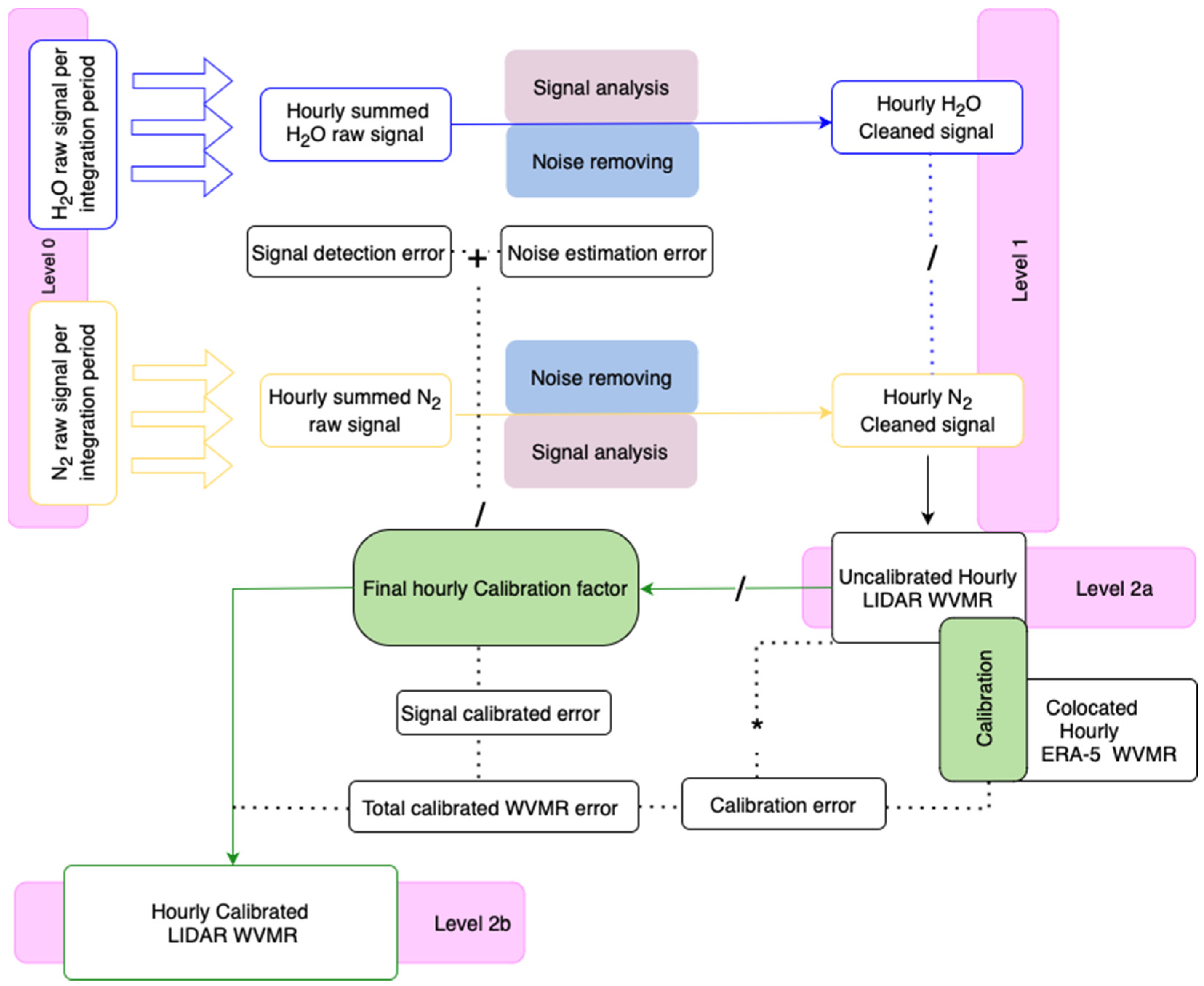
4. WVMR Lidar Treatment Channel and Calibration
4.1. WVMR
4.1.1. Signal Analyses
4.1.2. WVMR Error Estimation
- Calibrated Detection Error: The detection error (Appendix A), representing the uncertainty in detecting and quantifying the WVMR signal, is calibrated to reflect the scaling factors for this hour.
- Calibrated Noise Error: The noise estimation error (Appendix A) is first calibrated to account for any scaling factors. This calibration process adjusts the noise error for the hour based on the corresponding calibration factor.
- Calibration Error: This error accounts for any discrepancies or inaccuracies in the calibration procedure, impacting the final WVMR estimation.
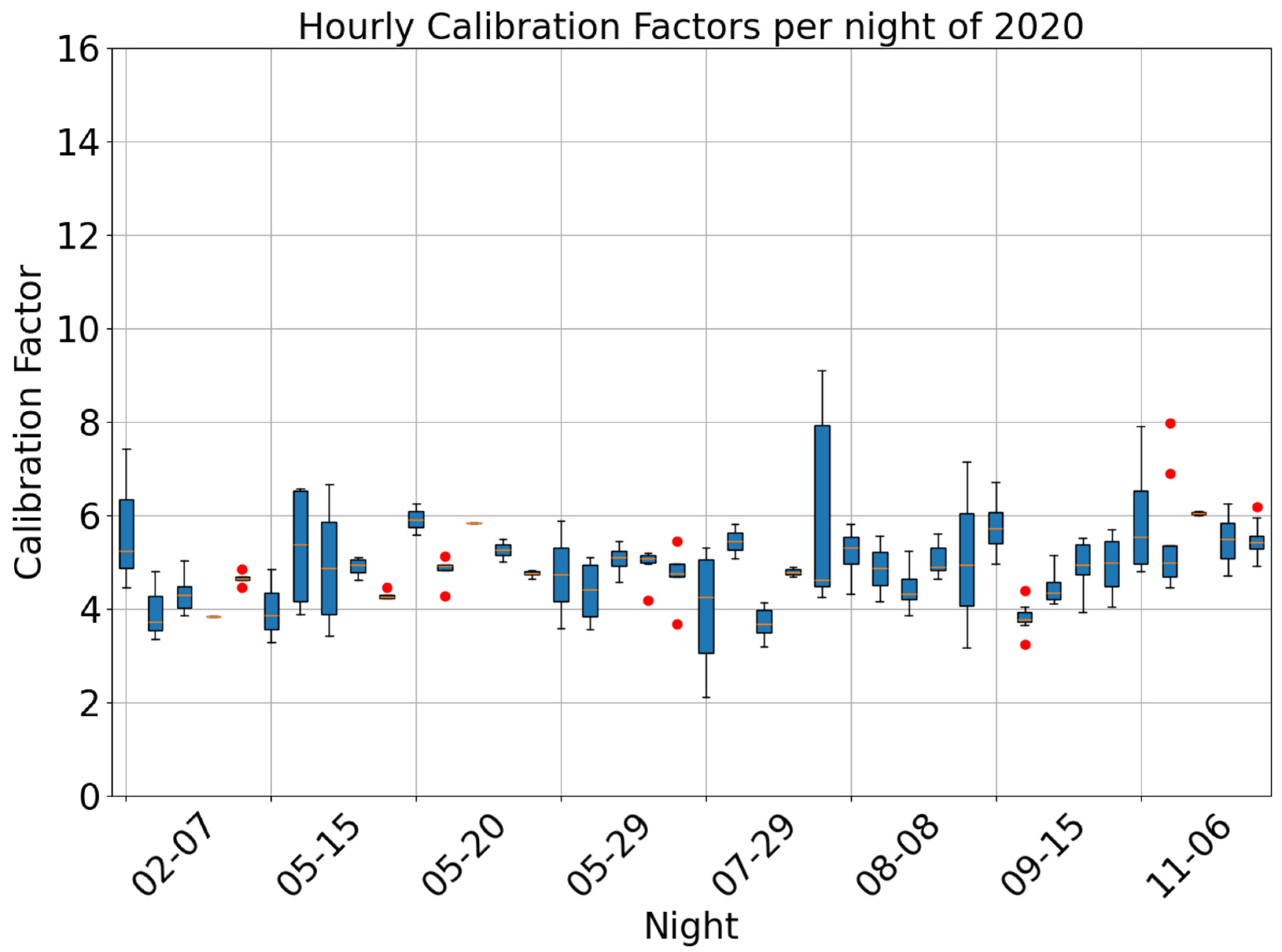
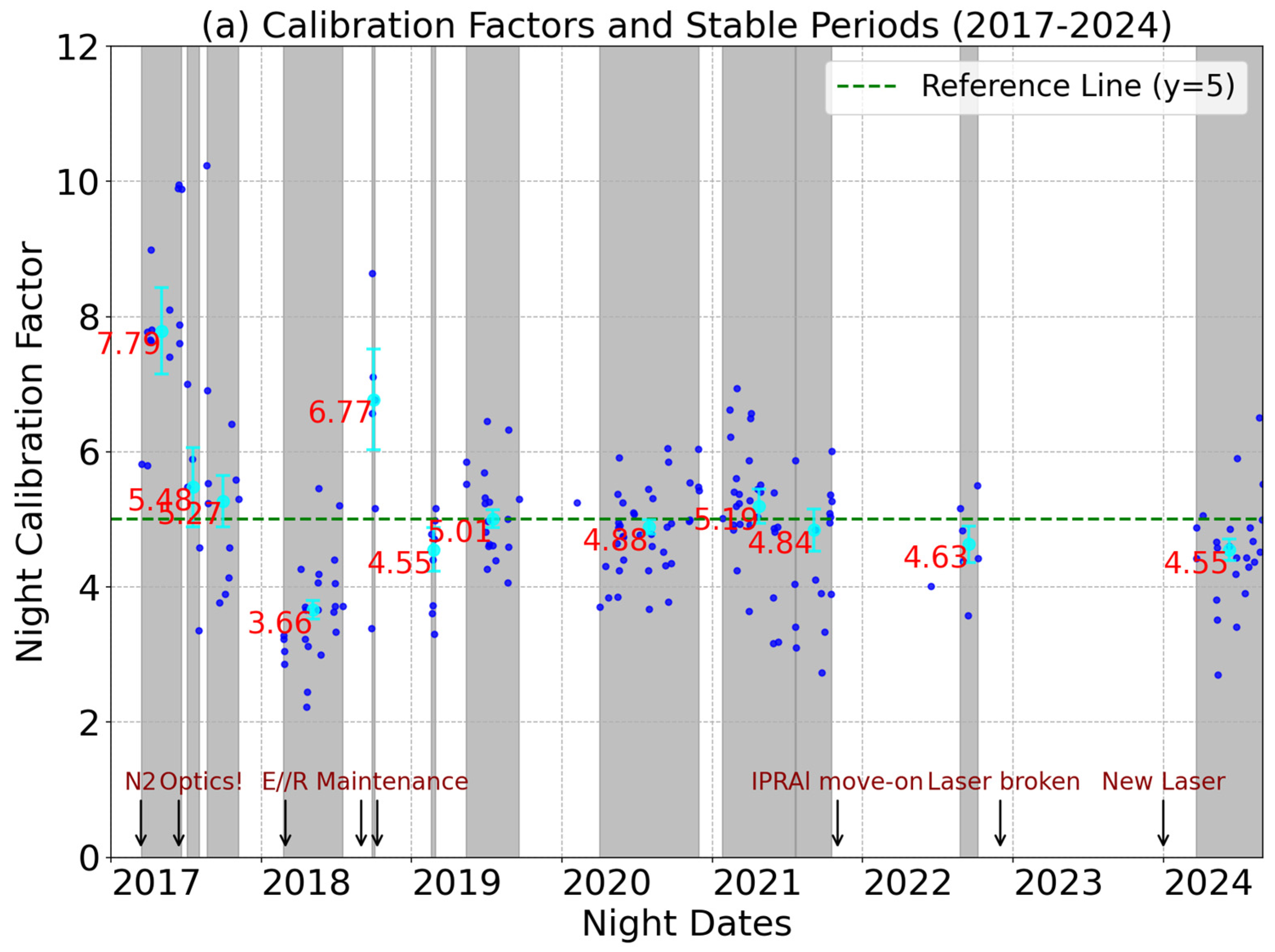
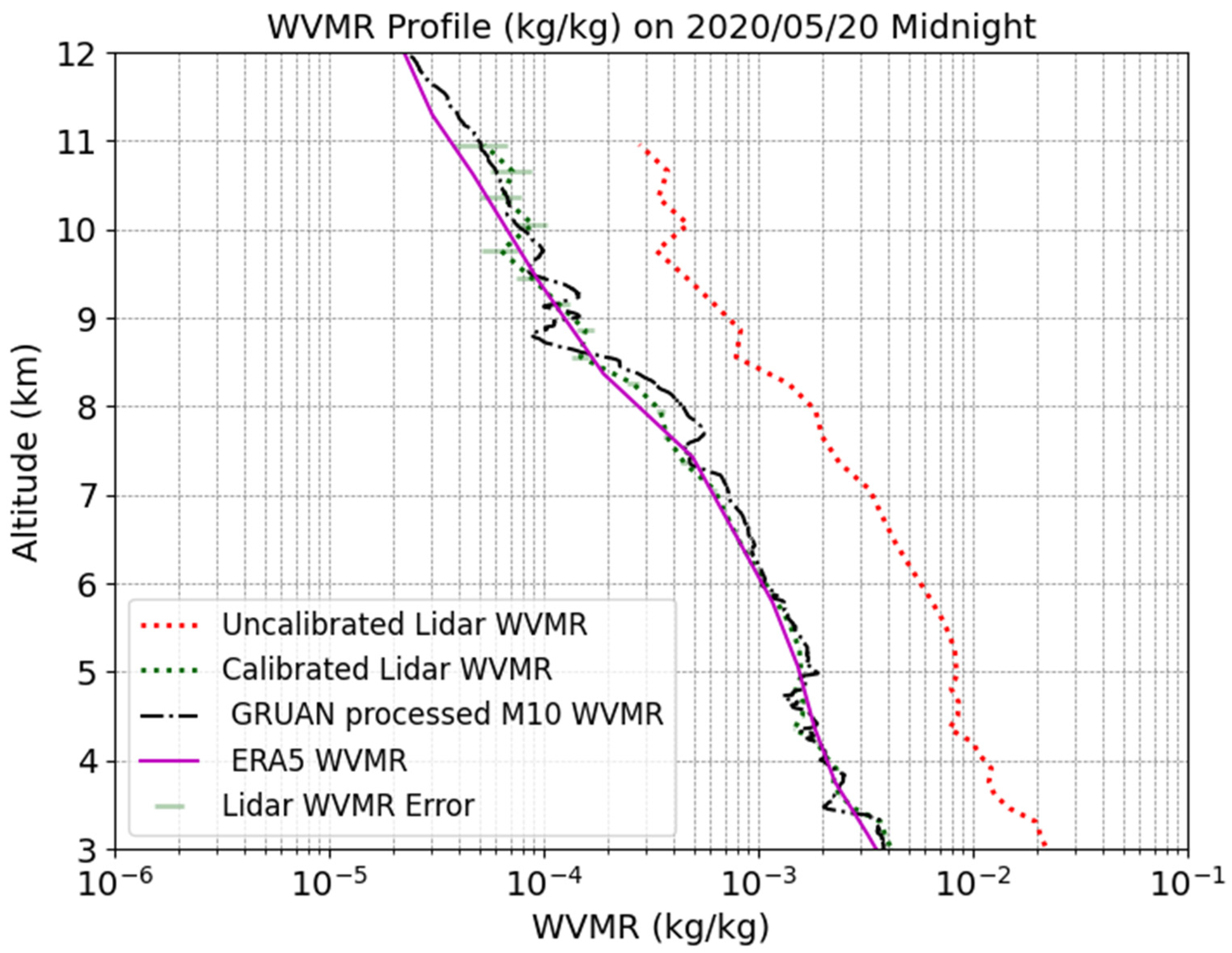
4.2. WVMR Calibration
5. Lidar Comparison with Other Datasets
5.1. Strategy
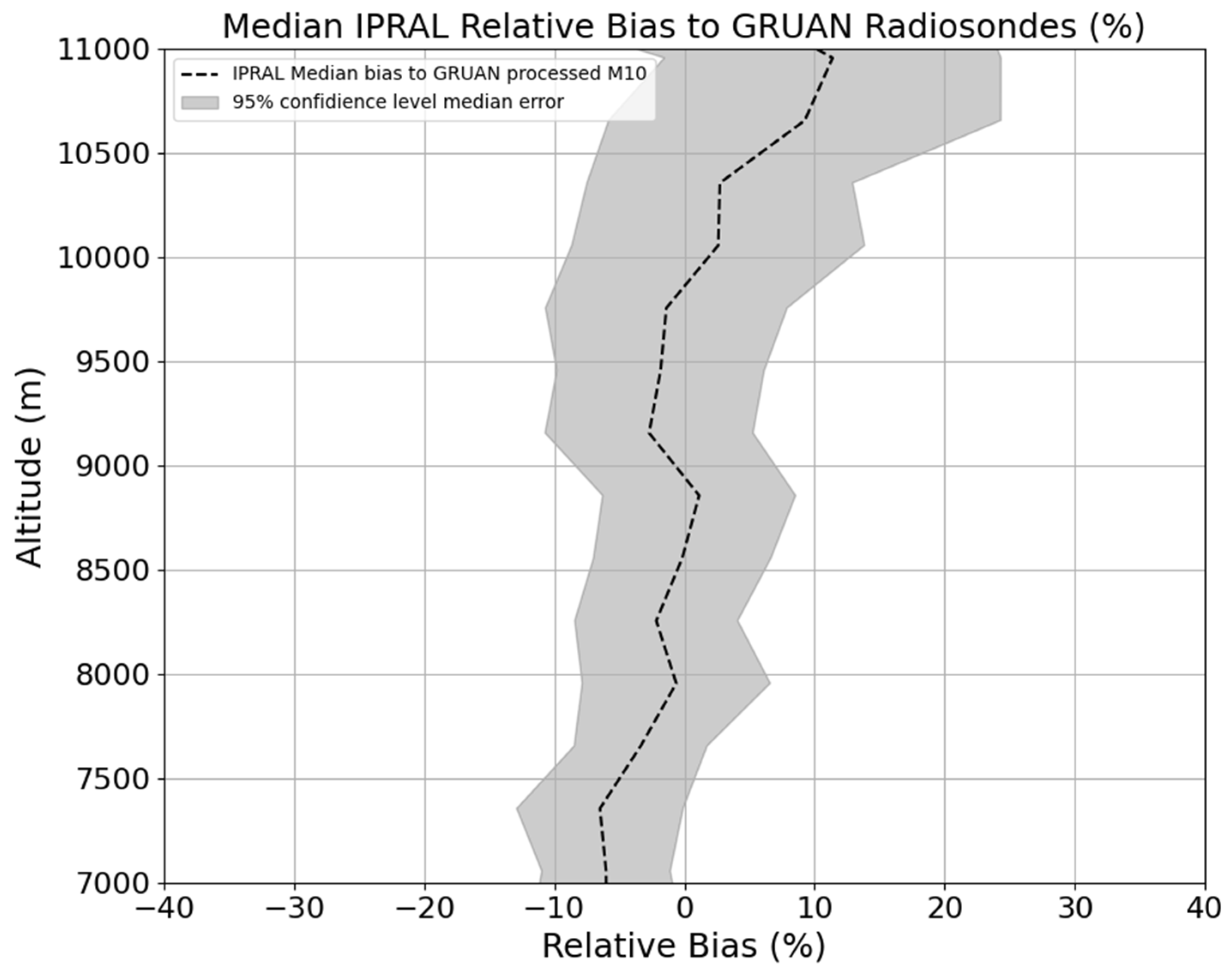
5.2. Lidar vs. RS
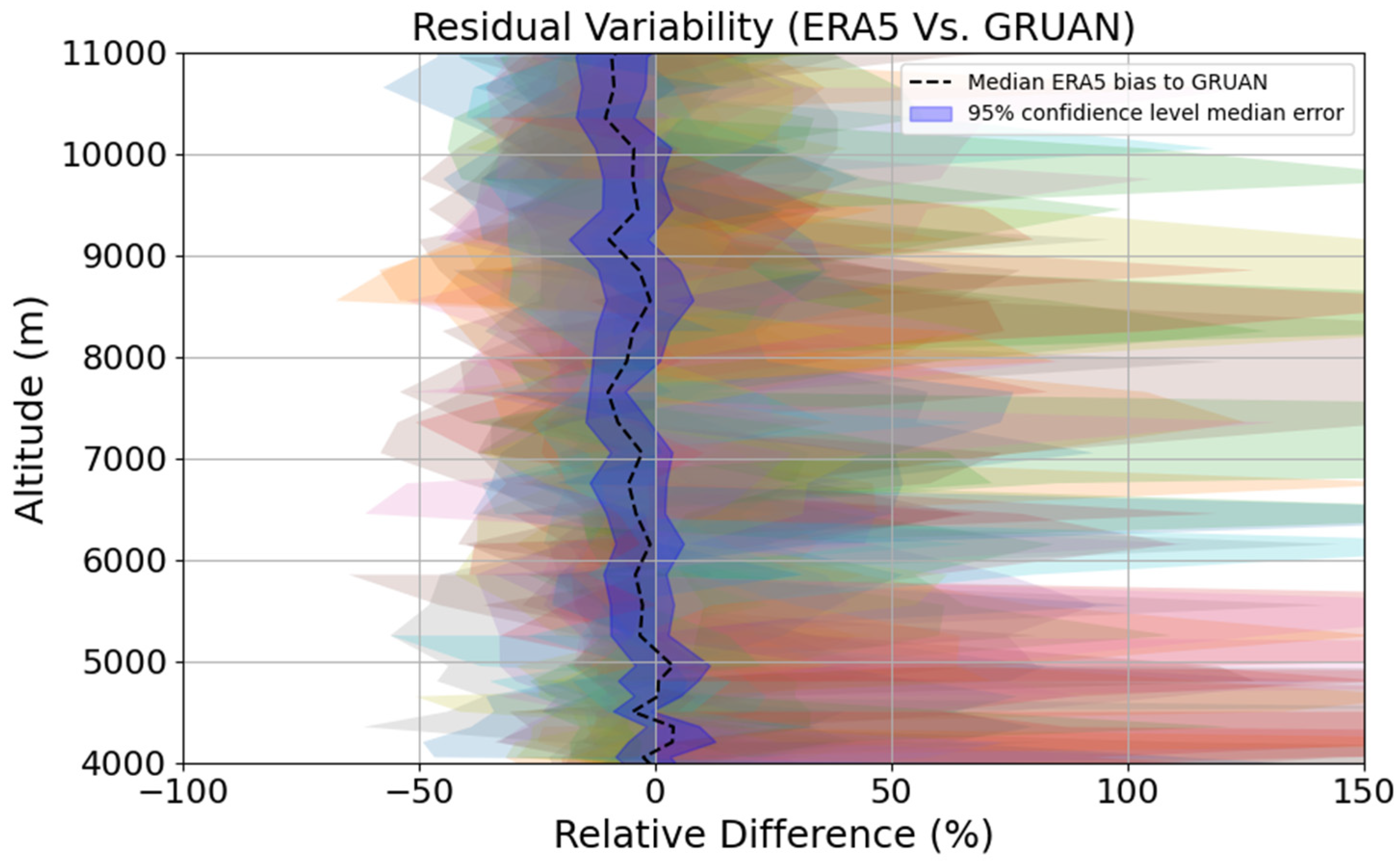
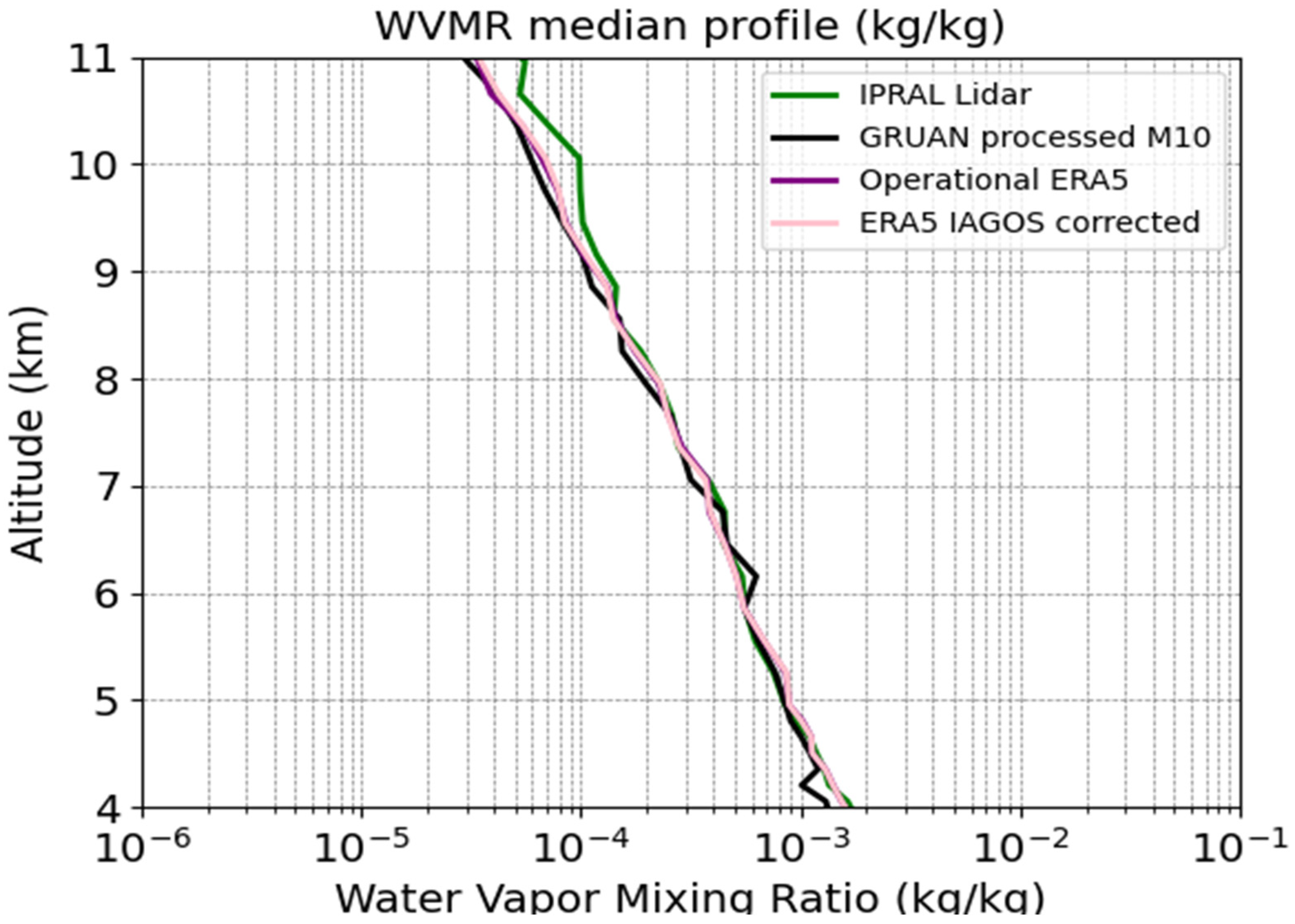
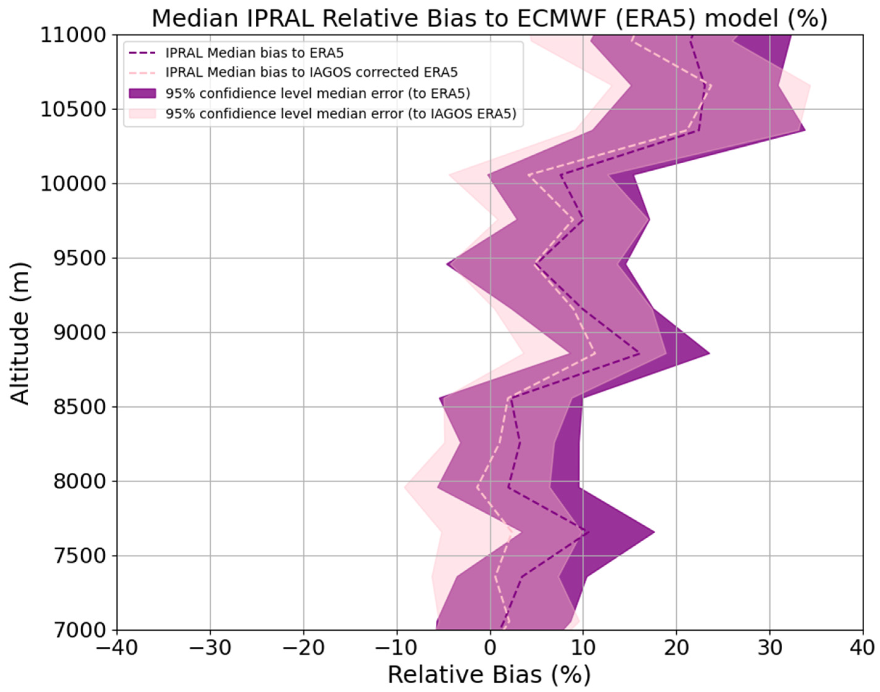
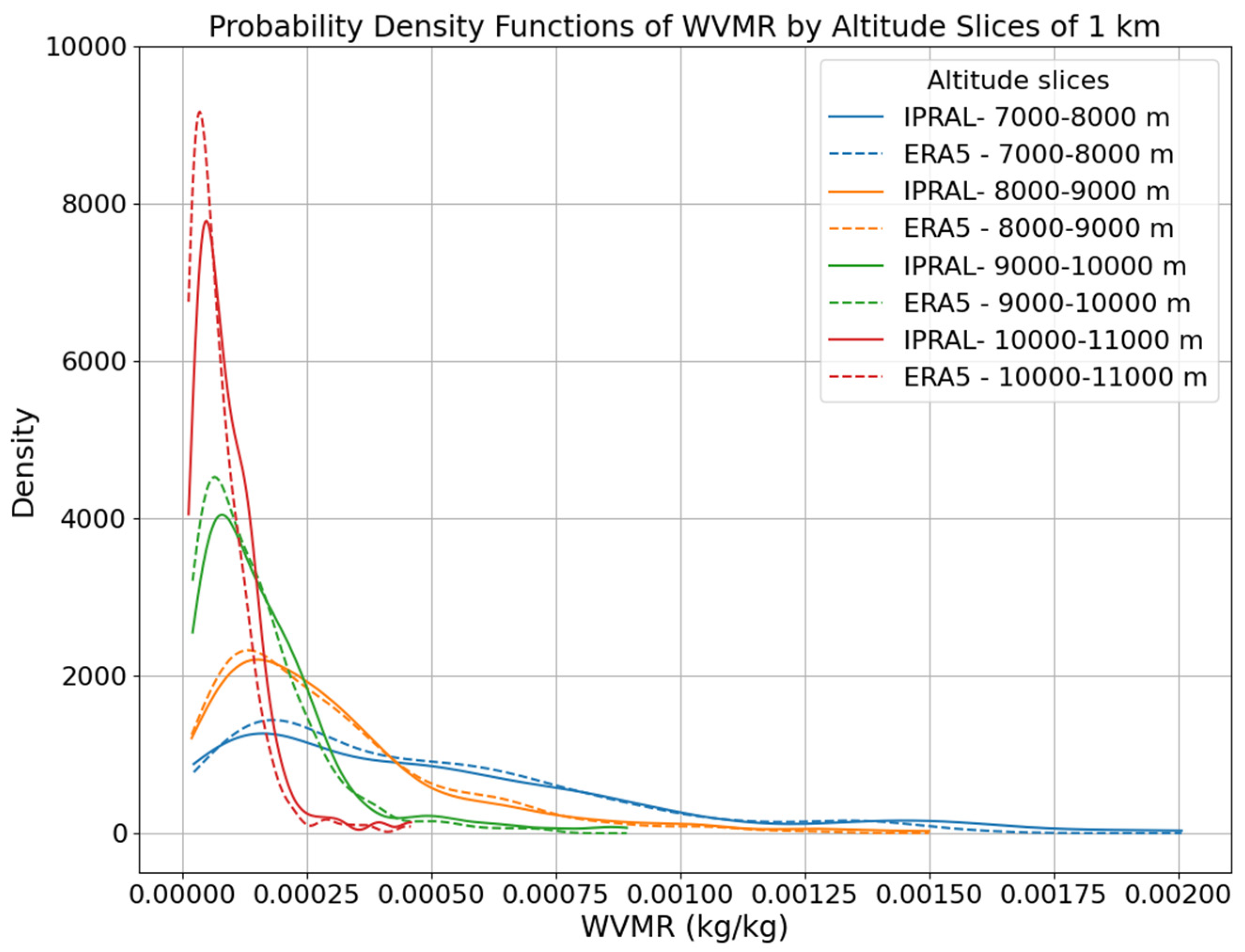
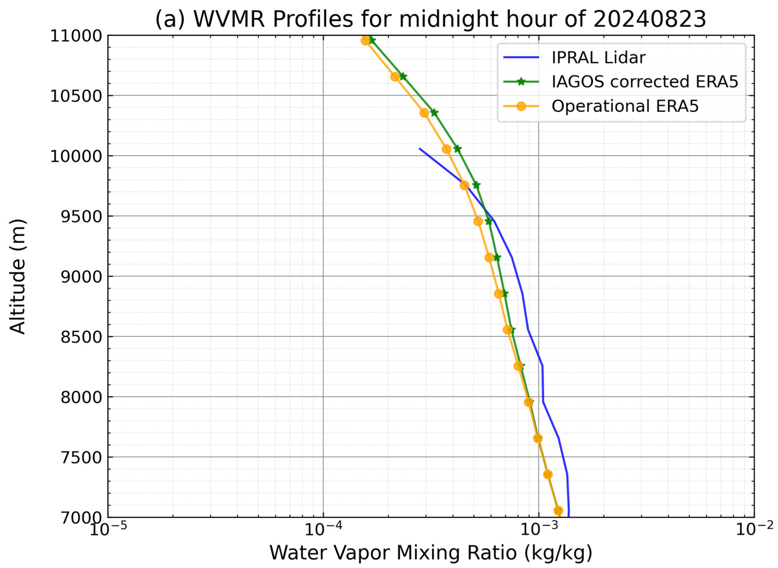
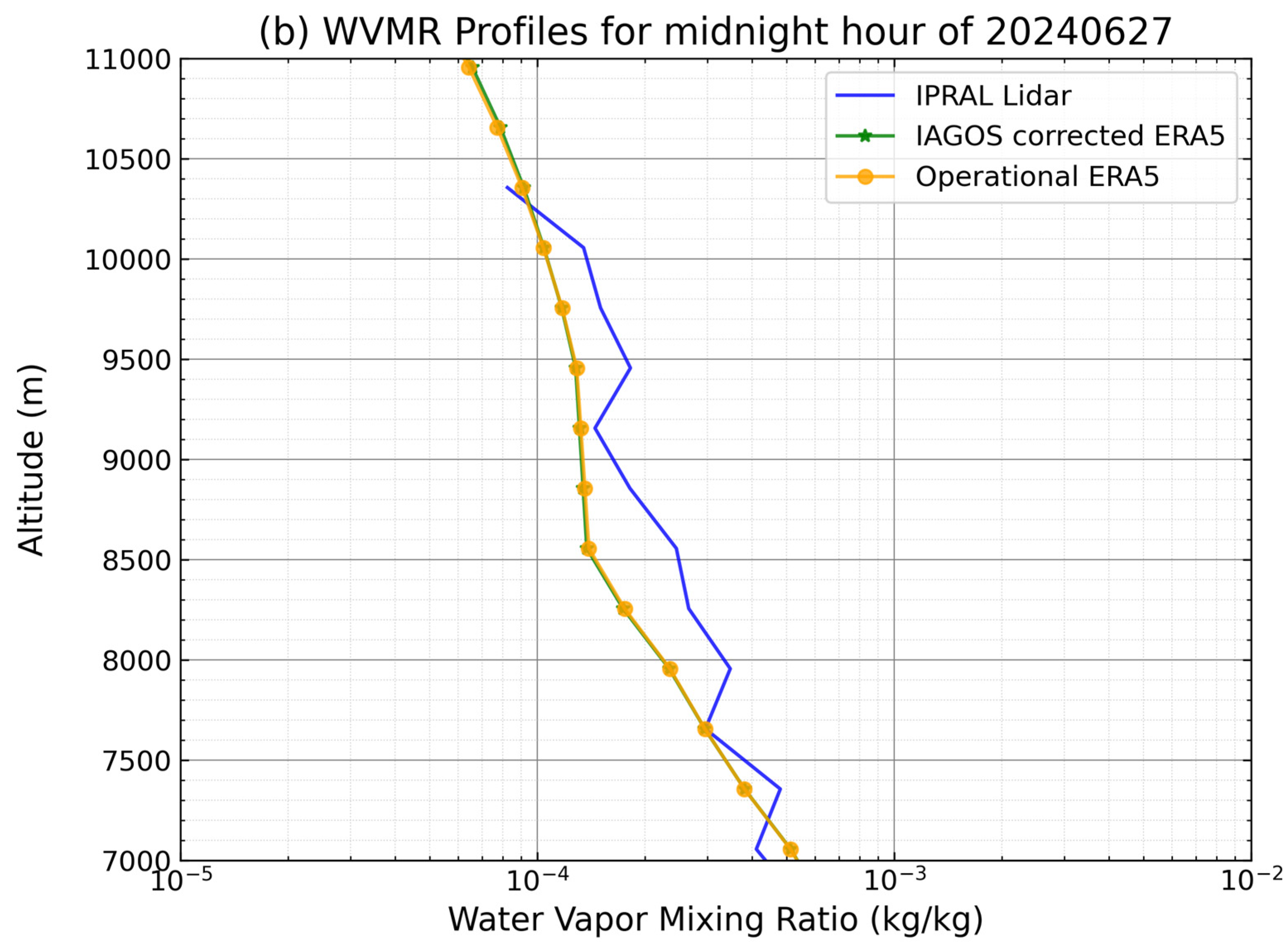
5.3. Lidar vs. ERA5
6. Discussion
7. Conclusions
- Calibration Reference: ERA5 was successfully used as the calibration reference, with GRUAN radiosonde data confirming its reliability for this purpose.
- Consistency with GRUAN: IPRAL Lidar shows biases of −5% to +10% relative to GRUAN analysed radiosondes, improving with altitude.
- ERA5 Bias: A dry bias of 10–20% in ERA5 relative to IPRAL. This bias might be partially consistent with known underestimations of humidity in ice-supersaturation regions, but it also seemed to be linked to systematic ERA5 bias over upper tropospheric altitudes.
- Improved ERA5 with IAGOS: The IAGOS-corrected ERA5 data set reduces biases and variability, validating its corrections and demonstrating the value of in situ data.
- Lidar Sensitivity: Raman Lidar’s ability to capture humidity variability, especially under supersaturated conditions, complements traditional radiosonde and ERA5 data.
Author Contributions
Funding
Institutional Review Board Statement
Informed Consent Statement
Data Availability Statement
Acknowledgments
Conflicts of Interest
Appendix A
- 1.
- Signal Detection Error
- 2.
- Noise Detection Error
- 3.
- Calibration Error
References
- Gierens, K.; Sausen, R.; Bauder, U.; Eckel, G.; Großmann, K.; Le Clercq, P.; Lee, D.S.; Rauch, B.; Sauer, D.; Voigt, C.; et al. Influence of aviation fuel composition on the formation and lifetime of contrails—A literature review. CONCAWE Rep. 2024, 24, 1–91. [Google Scholar]
- Teoh, R.; Schumann, U.; Gryspeerdt, E.; Shapiro, M.; Molloy, J.; Koudis, G.; Voigt, C.; Stettler, M.E.J. Aviation contrail climate effects in the North Atlantic from 2016 to 2021. Atmos. Chem. Phys. 2022, 22, 10919–10935. [Google Scholar] [CrossRef]
- Bock, L.; Burkhardt, U. Contrail cirrus radiative forcing for future air traffic. Atmos. Chem. Phys. 2019, 19, 8163–8174. [Google Scholar] [CrossRef]
- Singh, D.K.; Sanyal, S.; Wuebbles, D.J. Understanding the role of contrails and contrail cirrus in climate change: A global perspective. Atmos. Chem. Phys. 2024, 24, 9219–9262. [Google Scholar] [CrossRef]
- Irvine, E.A.; Shine, K.P. Ice supersaturation and the potential for contrail formation in a changing climate. Earth Syst. Dyn. 2015, 6, 555–568. [Google Scholar] [CrossRef]
- Wilhelm, L.; Gierens, K.; Rohs, S. Meteorological conditions that promote persistent contrails. Appl. Sci. 2022, 12, 4450. [Google Scholar] [CrossRef]
- Gierens, K.; Matthes, S.; Rohs, S. How well can persistent contrails be predicted? Aerospace 2020, 7, 169. [Google Scholar] [CrossRef]
- Sperber, D.; Gierens, K. Towards a more reliable forecast of ice supersaturation: Concept of a one-moment ice-cloud scheme that avoids saturation adjustment. Atmos. Chem. Phys. 2023, 23, 15609–15627. [Google Scholar] [CrossRef]
- Wolf, K.; Bellouin, N.; Boucher, O.; Rohs, S.; Li, Y. Correction of temperature and relative humidity biases in ERA5 by bivariate quantile mapping: Implications for contrail classification. EGUsphere 2023, 2023, 1–38. [Google Scholar]
- Thompson, G.; Scholzen, C.; O’Donoghue, S.; Haughton, M.; Jones, R.L.; Durant, A.; Farrington, C. On the fidelity of high-resolution numerical weather forecasts of contrail-favorable conditions. Atmos. Res. 2024, 311, 107663. [Google Scholar] [CrossRef]
- Petzold, A.; Neis, P.; Rütimann, M.; Rohs, S.; Berkes, F.; Smit, H.G.J.; Krämer, M.; Spelten, N.; Spichtinger, P.; Nédélec, P.; et al. Ice-supersaturated air masses in the northern mid-latitudes from regular in situ observations by passenger aircraft: Vertical distribution, seasonality and tropospheric fingerprint. Atmos. Chem. Phys. 2020, 20, 8157–8179. [Google Scholar] [CrossRef]
- Winker, D.M.; Pelon, J.R.; McCormick, M.P. CALIPSO mission: Spaceborne lidar for observation of aerosols and clouds. In Lidar Remote Sensing for Industry and Environment Monitoring III; SPIE: Bellingham, WA, USA, 2003; pp. 1–11. [Google Scholar]
- Dekoutsidis, G.; Groß, S.; Wirth, M.; Krämer, M.; Rolf, C. Characteristics of supersaturation in midlatitude cirrus clouds and their adjacent cloud-free air. Atmos. Chem. Phys. 2023, 23, 3103–3117. [Google Scholar]
- Keckhut, P.; Borchi, F.; Bekki, S.; Hauchecorne, A.; SiLaouina, M. Cirrus classification at midlatitude from systematic lidar observations. J. Appl. Meteorol. Clim. 2006, 45, 249–258. [Google Scholar]
- Groß, S.; Jurkat-Witschas, T.; Li, Q.; Wirth, M.; Urbanek, B.; Krämer, M.; Weigel, R.; Voigt, C. Investigating an indirect aviation effect on mid-latitude cirrus clouds–linking lidar derived optical properties to in-situ measurements. Atmos. Chem. Phys. Discuss. 2022, 23, 8369–8381. [Google Scholar]
- Mandija, F.; Keckhut, P.; Alraddawi, D.; Khaykin, S.; Sarkissian, A. Climatology of Cirrus Clouds over Observatory of Haute-Provence (France) Using Multivariate Analyses on Lidar Profiles. Atmosphere 2024, 15, 1261. [Google Scholar] [CrossRef]
- Hoareau, C.; Keckhut, P.; Baray, J.L.; Robert, L.; Courcoux, Y.; Porteneuve, J.; Vömel, H.; Morel, B. A Raman lidar at La Reunion (20.8 S, 55.5 E) for monitoring water vapour and cirrus distributions in the subtropical upper troposphere: Preliminary analyses and description of a future system. Atmos. Meas. Tech. 2012, 5, 1333–1348. [Google Scholar]
- De Rosa, B.; Di Girolamo, P.; Summa, D. Temperature and water vapour measurements in the framework of the Network for the Detection of Atmospheric Composition Change (NDACC). Atmos. Meas. Tech. 2020, 13, 405–427. [Google Scholar] [CrossRef]
- Leblanc, T.; McDermid, I.S.; Walsh, T.D. Ground-based water vapor Raman lidar measurements up to the upper troposphere and lower stratosphere—Part 2: Data analysis and calibration for long-term monitoring. Atmos. Meas. Tech. Discuss. 2011, 4, 5111–5145. [Google Scholar]
- Dionisi, D.; Keckhut, P.; Courcoux, Y.; Hauchecorne, A.; Porteneuve, J.; Baray, J.L.; de Bellevue, J.L.; Vérèmes, H.; Gabarrot, F.; Payen, G.; et al. Water vapor observations up to the lower stratosphere through the Raman lidar during the Maïdo Lidar Calibration Campaign. Atmos. Meas. Tech. 2015, 8, 1425–1445. [Google Scholar] [CrossRef]
- Venable, D.D.; Whiteman, D.N.; Calhoun, M.N.; Dirisu, A.O.; Connell, R.M.; Landulfo, E. Lamp mapping technique for independent determination of the water vapor mixing ratio calibration factor for a Raman lidar system. Appl. Opt. 2011, 50, 4622–4632. [Google Scholar]
- Leblanc, T.; McDermid, I.S.; Walsh, T.D. Ground-based water vapor Raman lidar measurements up to the upper troposphere and lower stratosphere for long-term monitoring. Atmos. Meas. Tech. 2012, 5, 17–36. [Google Scholar] [CrossRef]
- Dai, G.; Althausen, D.; Hofer, J.; Engelmann, R.; Seifert, P.; Bühl, J.; Mamouri, R.-E.; Wu, S.; Ansmann, A. Calibration of Raman lidar water vapor profiles by means of AERONET photometer observations and GDAS meteorological data. Atmos. Meas. Tech. 2018, 11, 2735–2748. [Google Scholar] [CrossRef]
- Vérèmes, H.; Payen, G.; Keckhut, P.; Duflot, V.; Baray, J.-L.; Cammas, J.-P.; Evan, S.; Posny, F.; Körner, S.; Bosser, P. Validation of the water vapor profiles of the raman lidar at the maïdo observatory (Reunion Island) calibrated with global navigation satellite system integrated water vapor. Atmosphere 2019, 10, 713. [Google Scholar] [CrossRef]
- Whiteman, D.N.; Russo, F.; Demoz, B.; Miloshevich, L.M.; Veselovskii, I.; Hannon, S.; Wang, Z.; Vömel, H.; Schmidlin, F.; Lesht, B.; et al. Analysis of Raman lidar and radiosonde measurements from the AWEX-G field campaign and its relation to Aqua validation. J. Geophys. Res. Atmos. 2006, 111, D09S09. [Google Scholar] [CrossRef]
- Leblanc, T.; McDermid, I.S. Accuracy of Raman lidar water vapor calibration and its applicability to long-term measurements. Appl. Opt. 2008, 47, 5592–5603. [Google Scholar] [CrossRef] [PubMed]
- Adam, M.; Demoz, B.B.; Venable, D.D.; Joseph, E.; Connell, R.; Whiteman, D.N.; Gambacorta, A.; Wei, J.; Shephard, M.W.; Miloshevich, L.M.; et al. Water vapor measurements by Howard University Raman lidar during the WAVES 2006 campaign. J. Atmos. Ocean. Technol. 2010, 27, 42–60. [Google Scholar] [CrossRef]
- Herold, C.; Althausen, D.; Müller, D.; Tesche, M.; Seifert, P.; Engelmann, R.; Flamant, C.; Bhawar, R.; Di Girolamo, P. Comparison of Raman lidar observations of water vapor with COSMO-DE forecasts during COPS 2007. Weather Forecast. 2011, 26, 1056–1066. [Google Scholar] [CrossRef]
- Bock, O.; Bosser, P.; Bourcy, T.; David, L.; Goutail, F.; Hoareau, C.; Keckhut, P.; Legain, D.; Pazmino, A.; Pelon, J.; et al. Accuracy assessment of water vapour measurements from in-situ and remote sensing techniques during the DEMEVAP 2011 campaign at OHP. Atmos. Meas. Tech. Discuss. 2013, 6, 3439–3509. [Google Scholar] [CrossRef]
- Totems, J.; Chazette, P. Calibration of a water vapour Raman lidar with a kite-based humidity sensor. Atmos. Meas. Tech. 2016, 9, 1083–1094. [Google Scholar] [CrossRef]
- Dirksen, R.J.; Bodeker, G.E.; Thorne, P.W.; Merlone, A.; Reale, T.; Wang, J.; Hurst, D.F.; Demoz, B.B.; Gardiner, T.D.; Ingleby, B.; et al. Managing the transition from Vaisala RS92 to RS41 radiosondes within the Global Climate Observing System Reference Upper-Air Network (GRUAN): A progress report. Geosci. Instrum. Methods Data Syst. 2020, 9, 337–355. [Google Scholar] [CrossRef]
- Hicks-Jalali, S.; Sica, R.J.; Haefele, A.; Martucci, G. Calibration of a water vapour Raman lidar using GRUAN-certified radiosondes and a new trajectory method. Atmos. Meas. Tech. 2019, 12, 3699–3716. [Google Scholar]
- Hicks-Jalali, S.; Sica, R.J.; Martucci, G.; Barras, E.M.; Voirin, J.; Haefele, A. A Raman lidar tropospheric water vapour climatology and height-resolved trend analysis over Payerne, Switzerland. Atmos. Meas. Tech. 2020, 20, 9619–9640. [Google Scholar]
- Vömel, H.; David, D.E.; Smith, K. Accuracy of tropospheric and stratospheric water vapor measurements by the cryogenic frost point hygrometer: Instrumental details and observations. J. Geophys. Res. Atmos. 2007, 112, D08305. [Google Scholar] [CrossRef]
- Meyer, J.; Rolf, C.; Schiller, C.; Rohs, S.; Spelten, N.; Afchine, A.; Zöger, M.; Sitnikov, N.; Thornberry, T.D.; Rollins, A.W.; et al. Two decades of water vapor measurements with the FISH fluorescence hygrometer: A review. Atmos. Chem. Phys. 2015, 15, 8521–8538. [Google Scholar]
- Filioglou, M.; Nikandrova, A.; Niemelä, S.; Baars, H.; Mielonen, T.; Leskinen, A.; Brus, D.; Romakkaniemi, S.; Giannakaki, E.; Komppula, M. Profiling water vapor mixing ratios in Finland by means of a Raman lidar, a satellite and a model. Atmos. Meas. Tech. 2017, 10, 4303–4316. [Google Scholar]
- Haeffelin, M.; Barthès, L.; Bock, O.; Boitel, C.; Bony, S.; Bouniol, D.; Chepfer, H.; Chiriaco, M.; Cuesta, J.; Delanoë, J.; et al. SIRTA, a ground-based atmospheric observatory for cloud and aerosol research. In Annales Geophysicae; Copernicus GmbH: Göttingen, Germany, 2005; pp. 253–275. [Google Scholar]
- Hersbach, H.; Bell, B.; Berrisford, P.; Biavati, G.; Horányi, A.; Muñoz Sabater, J.; Nicolas, J.; Peubey, C.; Radu, R.; Rozum, I.; et al. ERA5-Hourly Data on Model Levels, ECMWF [Data Set]; ECMWF: Reading, UK, 2023. [Google Scholar]
- Sherlock, V.; Garnier, A.; Hauchecorne, A.; Keckhut, P. Implementation and validation of a Raman lidar measurement of middle and upper tropospheric water vapor. Appl. Opt. 1999, 38, 5838–5850. [Google Scholar]
- Keckhut, P.; Chanin, M.L.; Hauchecorne, A. Stratosphere temperature measurement using Raman lidar. Appl. Opt. 1990, 29, 5182–5186. [Google Scholar]
- Seidel, D.J.; Berger, F.H.; Diamond, H.J.; Dykema, J.; Goodrich, D.; Immler, F.; Murray, W.; Peterson, T.; Sisterson, D.; Sommer, M.; et al. Reference Upper-Air Observations for Climate: Rationale, Progress, and Plans. Bull. Am. Meteorol. Soc. 2009, 90, 361–369. [Google Scholar] [CrossRef]
- Dupont, J.-C.; Haeffelin, M.; Badosa, J.; Clain, G.; Raux, C.; Vignelles, D. Characterization and corrections of relative humidity measurement from Meteomodem M10 radiosondes at midlatitude stations. J. Atmos. Ocean. Technol. 2020, 37, 857–871. [Google Scholar]
- Hersbach, H.; Bell, B.; Berrisford, P.; Hirahara, S.; Horányi, A.; Muñoz-Sabater, J.; Nicolas, J.; Peubey, C.; Radu, R.; Schepers, D.; et al. The ERA5 global reanalysis. Q. J. R. Meteorol. Soc. 2020, 146, 1999–2049. [Google Scholar]
- Petzold, A.; Thouret, V.; Gerbig, C.; Zahn, A.; Brenninkmeijer, C.A.M.; Gallagher, M.; Hermann, M.; Pontaud, M.; Ziereis, H.; Boulanger, D.; et al. Global-scale atmosphere monitoring by in-service aircraft—Current achievements and future prospects of the European Research Infrastructure IAGOS. Tellus B Chem. Phys. Meteorol. 2015, 67, 28452. [Google Scholar] [CrossRef]
- Hofer, S.; Gierens, K.; Rohs, S. How well can persistent contrails be predicted? An update. Atmos. Chem. Phys. 2024, 24, 7911–7925. [Google Scholar] [CrossRef]
- Hoareau, C.; Keckhut, P.; Sarkissian, A.; Baray, J.-L.; Durry, G. Methodology for water monitoring in the upper troposphere with Raman lidar at the Haute-Provence Observatory. J. Atmos. Ocean. Technol. 2009, 26, 2149–2160. [Google Scholar]
- Dinoev, T.; Simeonov, V.; Arshinov, Y.; Bobrovnikov, S.; Ristori, P.; Calpini, B.; Parlange, M.; van den Bergh, H. Raman lidar for meteorological observations, RALMO–Part 1: Instrument description. Atmos. Meas. Tech. 2013, 6, 1329–1346. [Google Scholar]
- Reichardt, J.; Wandinger, U.; Klein, V.; Mattis, I.; Hilber, B. and Begbie, R. RAMSES: German Meteorological Service autonomous Raman lidar for water vapor, temperature, aerosol, and cloud measurements. Appl. Opt. 2012, 51, 8111–8131. [Google Scholar]
- Di Girolamo, P.; De Rosa, B.; Flamant, C.; Summa, D.; Bousquet, O.; Chazette, P.; Totems, J.; Cacciani, M. Water vapor mixing ratio and temperature inter-comparison results in the framework of the Hydrological Cycle in the Mediterranean Experiment—Special Observation Period 1. Bull. Atmos. Sci. Technol. 2020, 1, 113–153. [Google Scholar]
- Reutter, P.; Neis, P.; Rohs, S.; Sauvage, B. Ice supersaturated regions: Properties and validation of ERA-Interim reanalysis with IAGOS in situ water vapour measurements. Atmos. Chem. Phys. 2020, 20, 787–804. [Google Scholar]


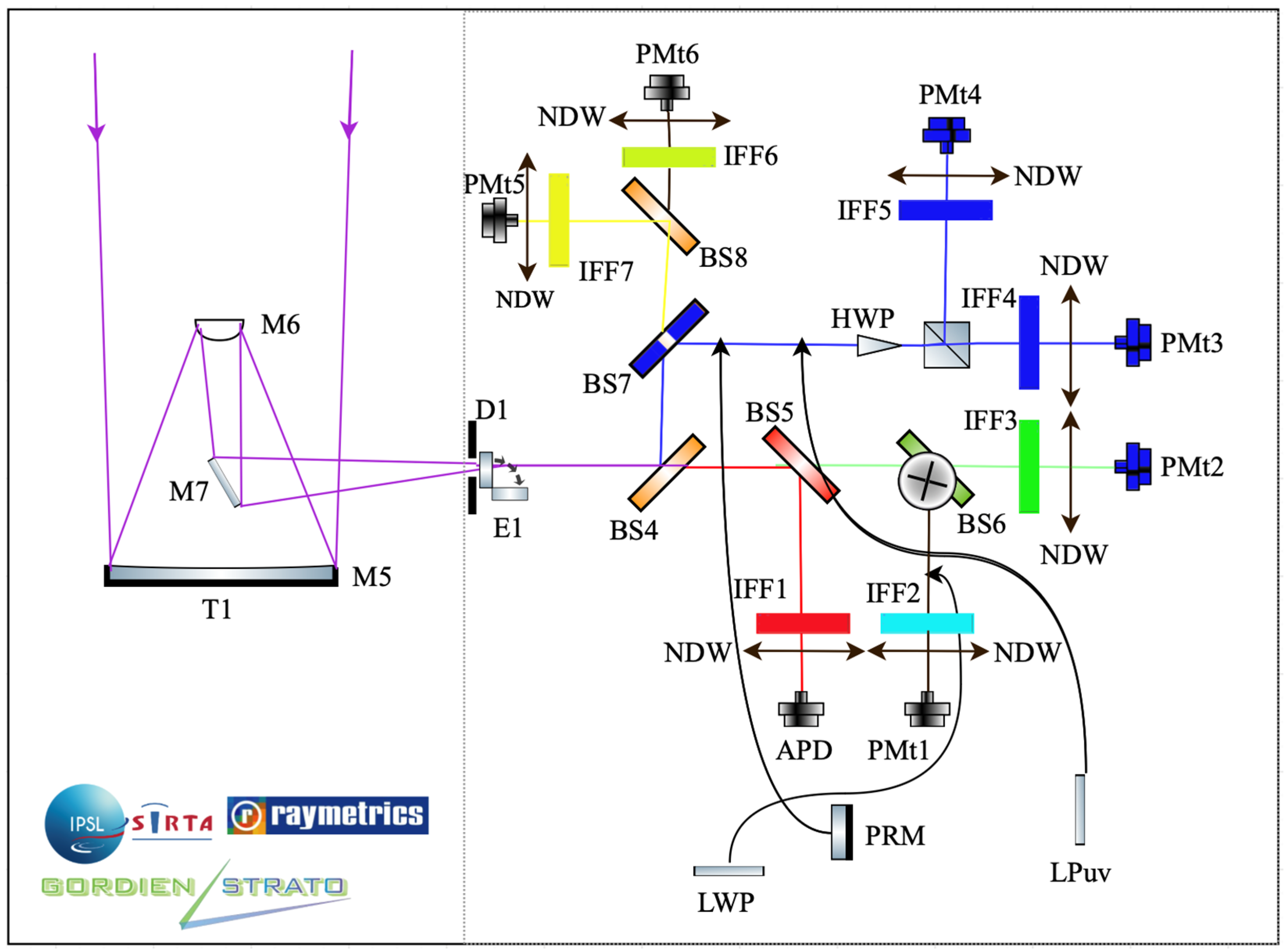
| Component | Long Name |
|---|---|
| Receiver tools | T1: Telescope 60 cm |
| M5: Elliptical Mirror | |
| M6: Spherical Mirror | |
| M7: Tertiary Plan Mirror | |
| Beam Splitters | BS4: Beam Splitter 532/532 nm |
| BS5: Beam Splitter 1064/1064 nm | |
| BS6: Beam Splitter 607/532 nm | |
| BS7: Beam Splitter 355/355 nm | |
| BS8: Beam Splitter 387/408 nm | |
| Interference Filters | IFF1: Interference Filter 1064.44 nm |
| IFF2: Interference Filter 607.48 nm | |
| IFF3: Interference Filter 532.26 nm | |
| IFF4: Interference Filter 354.75 nm | |
| IFF5: Interference Filter 354.75 nm | |
| IFF6: Interference Filter 407.59 nm | |
| IFF7: Interference Filter 386.67 nm | |
| Photomultipliers | PMt1: Photomultiplier 607 nm |
| PMt5: Photomultiplier 387 nm | |
| PMt6: Photomultiplier 408 nm | |
| PMt2: Gated Photomultiplier 532 nm | |
| PMt3: Gated Photomultiplier 355 nm | |
| PMt4: Gated Photomultiplier 355 nm | |
| Divers | NDW: Neutral Density Wheel (6 position, see Figure 1) |
| HWP: Half Wave Plate | |
| LPuv: Linear Ultraviolet Polarizer | |
| PRM: Partial Reflecting Mirror | |
| LWP: Long Wave Pass Optical Edge Filter |
Disclaimer/Publisher’s Note: The statements, opinions and data contained in all publications are solely those of the individual author(s) and contributor(s) and not of MDPI and/or the editor(s). MDPI and/or the editor(s) disclaim responsibility for any injury to people or property resulting from any ideas, methods, instructions or products referred to in the content. |
© 2025 by the authors. Licensee MDPI, Basel, Switzerland. This article is an open access article distributed under the terms and conditions of the Creative Commons Attribution (CC BY) license (https://creativecommons.org/licenses/by/4.0/).
Share and Cite
Alraddawi, D.; Keckhut, P.; Mandija, F.; Sarkissian, A.; Pietras, C.; Dupont, J.-C.; Farah, A.; Hauchecorne, A.; Porteneuve, J. Calibration of Upper Air Water Vapour Profiles Using the IPRAL Raman Lidar and ERA5 Model Results and Comparison to GRUAN Radiosonde Observations. Atmosphere 2025, 16, 351. https://doi.org/10.3390/atmos16030351
Alraddawi D, Keckhut P, Mandija F, Sarkissian A, Pietras C, Dupont J-C, Farah A, Hauchecorne A, Porteneuve J. Calibration of Upper Air Water Vapour Profiles Using the IPRAL Raman Lidar and ERA5 Model Results and Comparison to GRUAN Radiosonde Observations. Atmosphere. 2025; 16(3):351. https://doi.org/10.3390/atmos16030351
Chicago/Turabian StyleAlraddawi, Dunya, Philippe Keckhut, Florian Mandija, Alain Sarkissian, Christophe Pietras, Jean-Charles Dupont, Antoine Farah, Alain Hauchecorne, and Jacques Porteneuve. 2025. "Calibration of Upper Air Water Vapour Profiles Using the IPRAL Raman Lidar and ERA5 Model Results and Comparison to GRUAN Radiosonde Observations" Atmosphere 16, no. 3: 351. https://doi.org/10.3390/atmos16030351
APA StyleAlraddawi, D., Keckhut, P., Mandija, F., Sarkissian, A., Pietras, C., Dupont, J.-C., Farah, A., Hauchecorne, A., & Porteneuve, J. (2025). Calibration of Upper Air Water Vapour Profiles Using the IPRAL Raman Lidar and ERA5 Model Results and Comparison to GRUAN Radiosonde Observations. Atmosphere, 16(3), 351. https://doi.org/10.3390/atmos16030351