Abstract
Using the same initial condition in vortex merger, the backward integrations of height and vorticity from Sun’s shallow water model are the images of forward integrations. The system becomes very stable after long forward or backward integration (integration time > 120). If we integrate forward in time from initial t = t0 to t = tf, then, use the result as the initial condition to integrate backward from tf to t0. The difference between backward integration and the forward initial system at t = t0 increases as integration time increases. The difference is small if tf is less than 40 and backward integration can retrieve the original initial pattern well. If tf > 60, the difference becomes noticeable and the backward integration cannot retrieve the original pattern because of the accumulation of small difference generated at each time-step between forward and backward numerical calculations. The reverse time can be extended using implicit schemes or more complicated time-step schemes.
1. Introduction
The inverse problem has been important in numerical weather prediction, mathematics, physics, geoscience, engineering, medicine, environment, and other areas. Many inverse problems are related to the Navier–Stokes equations, which consist of nonlinear partial differential equations (PDEs) and are difficult to solve. For some wave type equations, scientists have successfully converted the partial differential equations to the integrable differential equations. Boussinesq [1] introduced several simple nonlinear systems of PDEs to explain certain water waves, including the Korteweg–de Vries equation [2].
For a fixed wave type solution , where c is phase speed and is an arbitrary constant, Equation (1) can be converted to an ordinary differential equation (ODE).
Korteweg and de Vries [3] obtained the analytic solitary solution.
The solitary waves propagate at a fixed phase speed, without change in shape through a delicate balance between linear wave dynamics and weak nonlinearity. The kdV and modified KdV equations are important to shallow water equation (SWE), acoustic waves on a crystal lattice, other physics problems, etc. [2]. Bäcklund transform was applied to solving SWE and others by finding the relationship between the solutions of the original PDE and the known solutions of KdV, Burgers equation, sine-Gordon equation, etc. [4,5,6,7,8]. Hu and Chen [9] applied Bäcklund transform to study the weak nonlinear quasi-geostrophic potential vorticity (QGPV) equation. The Bäcklund transformations can be a useful method to solve equations of soliton solutions, but no systematic way of finding Bäcklund transforms is known [6]. Perturbation and asymptotic analysis were also applied for solving the nonlinear PDE in fluid dynamics. The formulation of the governing equations contains small parameters which are used in asymptotic expansions of the variables [10,11]. Based on asymptotic analysis, Boyd [12,13] showed that the Equatorial solitary Rossby wave in a beta plane can be presented by the KdV equation. Unfortunately, not every nonlinear problem has such kinds of perturbation quantity. In addition, even if there exists a small parameter, the sub-problem might have no solutions or might be complicated so that only a few of the sub-problems can be solved [14]. Hence, numerical methods are frequently used to solve the nonlinear PDE and Navier–Stokes equations.
It is well known that most fluid dynamics models require artificial smoothing/filter to control nonlinear instability. The Navier–Stokes equations are usually integrated forward in time instead of backward in time because backward integration of diffusion equations may result in exponential growth [15], and nonlinear instability can be more vulnerable in backward integration [16,17]. Traditionally, people use time-consuming iterative approaches to solve inverse problems [18]. In order to overcome those challenges, Sun developed the numerical methods solving the inverse diffusion equation and the shallow water model that we can integrate the Equatorial Rossby solitary waves forward and backward in time [19,20]. The numerical simulations reproduce the analytic solutions of the propagation of the wave and the detailed secondary circulation inside the soliton [12,13]. The inverse of Rossby wave also confirms a reversible dynamical process of KdV, which is a hyperbolic PDE [20]. It also proves the validity and reliability of backward integration of Sun’s model. Here, we will integrate Sun’s model [21] backward to study the inverse of vortices merging [22,23,24,25,26,27], in which the nonlinear terms are important, and the pattern changes drastically and is different from the weak nonlinear Rossby soliton. Sun [20] proposed that the system is reversible if the change in variable ψ satisfies d ψ(−t)= −d ψ(t), which is confirmed by the reverse of Rossby soliton, but is different from the Euler equations, which are reversible if the advection terms satisfy adv(u) = adv(−u) according to Duponcheel et al. [28]; or u(−t) = −u(t), suggested by Eckhardt and Hascoet [29] or Fang et al. [30]. Our numerical results confirm the reversibility of a vortex merger if the integration time is less than 60. If integration is greater than that, the simulations cannot retrieve the initial configuration. After long (t ≥ 90) forward or backward integration, the system which consists of a core surrounded by long filaments becomes very stable. The 1D simulated energy spectrum shows an inverse cascade with a slope of −2 existing in vortices merging, but the slope is steeper than −3 for shortwaves because of the inviscid fluid in a fast rotation frame.
2. Basic Equations and Numerical Model
The flux form of the shallow water equations can be written as follows:
where the water depth is h and the terrain surface height is hs. Thus, the free water surface height hf = h + hs, ψ = hu, = hv, u and v are x and y component velocities, respectively. The equations are solved using Sun’s scheme, which not only has neutral stability but also does not require physical or artificial smoothing/diffusion to control numerical instability. It was applied to the shockwave in dam-breaking [21], vortices moving over Taiwan complex mountains [31], vortices merging [27], etc., as discussed in Sun [32].
The model can be applied to both forward and backward integrations. According to Sun [20], in backward integration, we calculate from a given data set at the n + 1th time-step.
Then, we use , and to calculate and , i.e., the following occurs:
Finally, we solve the Coriolis force implicitly.
and
Equations (4)–(6) can be combined into the potential vorticity (Π) equation.
where relative vorticity , and potential vorticity , which is conserved following the movement of the parcel in an inviscid fluid.
3. Numerical Results
3.1. Case A: Initial Condition and Numerical Simulations
The domain consists of 480 × 480 grids, with dx = dy = 0.025. Following Waugh [23] and Sun and Oh [27], we set g = 1, do = 2, and the initial water height is the following:
where = 1, = −0.1, yo = 0, x1 = 1 (=40 dx), x2 = −1 (=−40 dx), and ro. = 1.2 (=48 dx). Geostrophic wind is also assumed initially. The initial speed (colormap) with a maximum of 0.159, potential vorticity (black contour) with a maximum of 1.476, height (red contour) with a minimum of 0.886, and stream function (white arrow) are presented in Figure 1a. It also shows that A and B are on the same contour of Π = 0.5 but different velocities. In forward integration, Figure 1b shows that the vortices rotate anticlockwise. The centers of the vortices move slightly farther away to northeast and southwest due to centrifugal force. The fluids at A and B on the contour of Π = 0.5 in Figure 1a move to the corresponding locations A and B in Figure 1b, respectively. The fluid at B not only moves faster but also curves and departs farther away from A, which lengthens the filament. Because the end of the filaments move much slower than at the root, the filament grows with time, as shown in Figure 1c, at t = 40 in forward integration. The potenital vorticy Π of the parcel is coserved (D Π/Dt = 0) in inviscid fluid, hence, the filaments cannot be ejected from the inner core of vortex where the potential vorticity is higher, although many scientists proposed that the formation of filaments comes from the ejection of vorticity from the core [22,25,26].
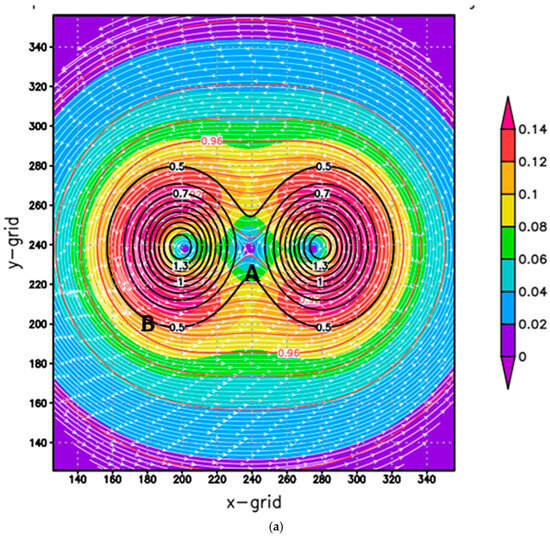
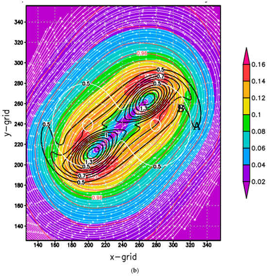
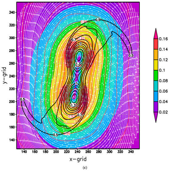
Figure 1.
(a) Speed (colormap) with maximum of 0.159; potential vorticity (black contour) with maximum of 1.476; height (red contour) with minimum of 0.886; and stream function (white arrow) at t = 0, and A and B at Π = 0.5 with different speeds. (b) Same as (a) but at t = 20 from forward integration. White contours outline vortices at t = 0, and fluid at A and B coming from A and B in (a), respectively. (c) Same as Figure 1a but at t = 40 from forward integration.
Starting from the same initial condition as in forward integration, Figure 2a shows the backward integration at t = −40. The stream functions show a counterclockwise circulation as in the forward integration. But the clockwise rotation of potential vorticity and height field in Figure 2a are the mirror images along the center line at x = 240 of the forward integration shown in Figure 1c.
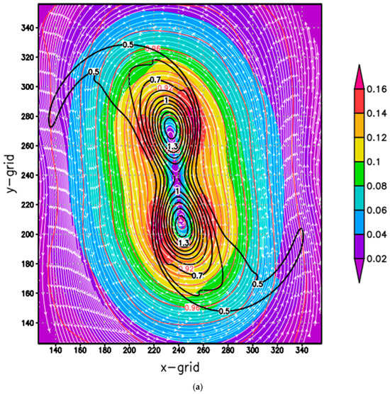
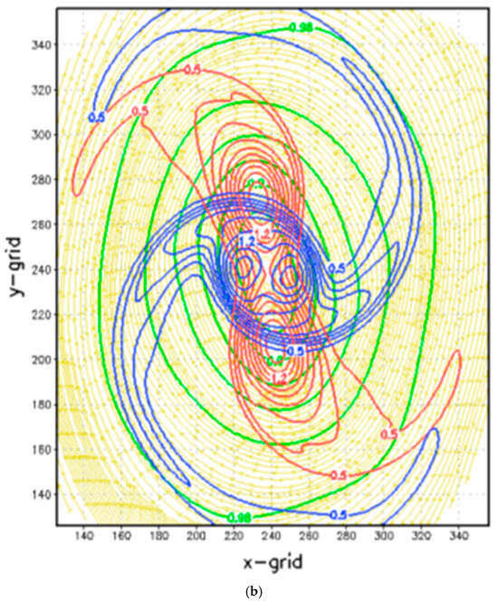
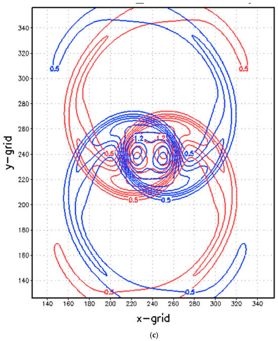
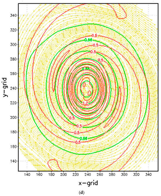
Figure 2.
(a) Same as Figure 1c but at t = −40 from backward integration. (b) Backward integrations of Π at t = −40 (red) and t = −80 (blue), and green contours mean height between t = −40 and t = −80. Sign of streamline changed from anticlockwise to clockwise. (c) Forward integration Π (red) at t = 80 and backward integration Π (blue) at t = −80. (d) Forward integration Π (red), height (green), and streamline (yellow) at t = 120.
Figure 2b shows the potenital vorticy Π at t = −40 (red), t= −80 (blue), the mean height (green), and the negative streamlines (yellow) between t = −40 and t = −80 because the clockwise rotation of vortices in backward integration can be interpreted by changing the sign of velocity according to . Here, we change the sign of mean velocity to show that the red shape at t = −40 moves to the blue one at t = −80 with negative velocity indicated by streamlines. The filaments lengthen with time due to velocity variation as well as shrink and erosion of the core border. In Navier–Stokes equations in rotating frame, the solution of backward integration cannot be obtained by just changing the velocity v from positive in forward integration to negative in backward integration.
but .
The inverse of fluid in the rotating system is different from those discussed by Duponcheel et al. [28], Eckhardt and Hascoet [29], Fang et al. [30], etc. The simulated streamlines remain as anticlockwise circulations for both forward (Figure 1c) and backward integrations (Figure 2a) instead of changing signs. A reflection between the forward integration at t = 80 and backward integration at t = −80 in Figure 2c further confirms that the scheme can be integrated forward and backward, and the simulation becomes the image of the other. They approach steady state after long integration (t > 90). The forward integration at t = 120 (Figure 2d) shows two distinguishable potential vorticity centers (red) near the center surrounded by long, narrow spiral filaments, and the lenth gradually increases with time. There is a broad concave height field with a minimum located at center.
The total mass (MA), energy (EN), potential vorticity (PV), and enstrophy (HE) are as follows:
and
Figure 3 shows the time sequences of the ratio of the variables with respect to their initial values from backward integration (they also present forward integration if time −t is replaced by t): MA(t)/MA(t = 0) by green, EN(t)/EN (t = 0) by red, PV(t)/PV(t = 0) by blue, and HE(t)/HE(t = 0) by black. They remain near a constant with respect to time in both integrations, although open boundary conditions are applied to this study. The total kinetic energy () slightly decays with time because of the truncation error and dispersion of phase speed among different wave lengths calculated from the fourth order differences scheme, and partially due to waves passing though lateral boundaries. The decay of KE also induces a slight decrease in total enstrophy (HE) through the change of , but less in total energy (EN), in which the potential energy is much larger than the kinetic energy.
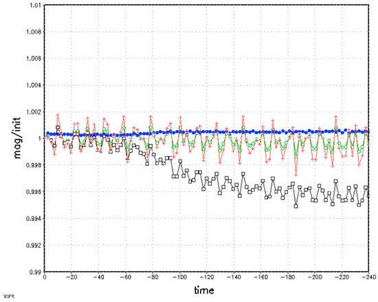
Figure 3.
Time sequence of total mass (MA), energy (EN), potential vorticity (PV), and enstrophy (HE) with respect to their initial values for backward integration.
3.2. Energy and Enstrophy
The energy en and enstrophy he in real space (m, n) can also be presented in spectra space .
The inverse discrete Fourier series are as follows:
The Fast Fourier Transform (FFT) developed by Miller [33] was used in this study. The numerical results show the sum (or integral) of the square of a function equal to the sum (or integral) of the square of its transform according to Parseval’s theorem.
and
The as functions of 2D wavenumber K and L at t = 0 in Figure 4a,b show that both decrease rapidly with the increase in wave number, especially along K. Both show the gap at K = 3, 9, and 15 at t = 0. Figure 4c,d show when the systems reach quasi-steady at t = ±120. It also shows that energy shifts toward longwave with for wavenumber ≤ 3 corresponding to the broadening area of the smooth height field in Figure 2d. Figure 4d reveals that the area of the vortex core is smaller than that of the energy, i.e., exists for wavenumber ≤ 7, and bands of extend to shortwaves because of long filaments, as shown in Figure 2d.
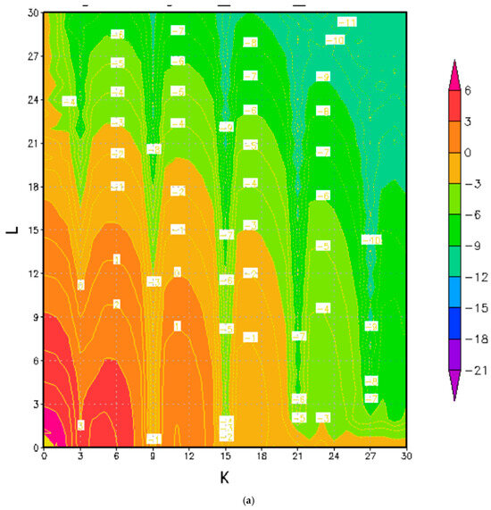
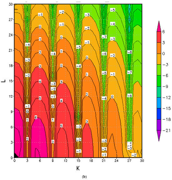

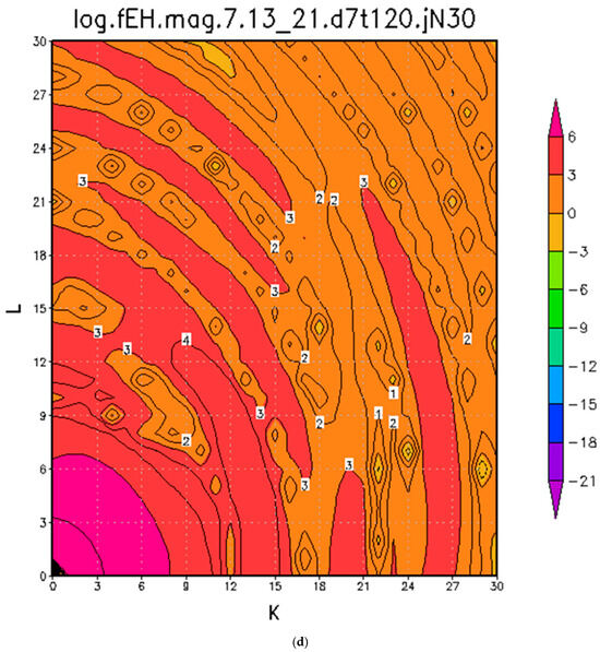
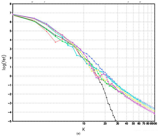
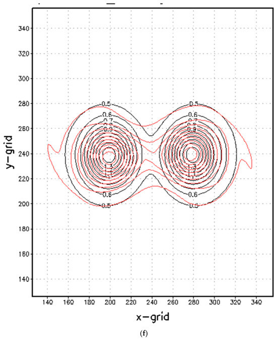
Figure 4.
(a) as function of wavenumber K and L at t = 0 for Case A. (b) as function of wavenumber K and L at t = 0 for Case A. (c) as function of wavenumber K and L at t = 120 for Case A. (d) as function of wavenumber K and L at t = 120 for Case A. (e) as function of 1D wavenumber K for Case A at t = 0 (black), t = 20 (red), t = 40 (green), t = 60 (blue), t = 80 (light blue), t = 120 (yellow), and t = 160 (purple). (f) Backward integration of Π at t = 0 (red) after 3100 time-steps from forward integration at t = 40 shown in Figure 2. Black contours are the initial Π at t = 0 in forward integration.
The energy E and enstrophy Z equations in turbulence flow are as follows:
where Kinetic energy ε is dissipation, and E and Z in physical space can also be presented by 1D spectra [34].
Kolmogorov [35] and Obukhov [36] proposed that in 3D turbulence, in inertia range satisfies the following:
where C~ 0.6. Equation (26) is based on the injected energy ε being transferred to short waves without dissipation in the inertia range. In a 2D flow, Batchelor [37] identified the cause of inverse energy transfer and simultaneous conservation of enstrophy and energy. He also predicted that the motion of the energy “centroid” will be toward larger scales because of the invariant of both total energy and enstrophy in the inertia range. Fjortoft [38] demonstrated that energy is not dissipated by viscosity and is dynamically transferred to large scales by the inverse cascade and enstrophy has a direct cascade to short waves. Batchelor [39] computed the energy spectrum in homogeneous two-dimensional turbulence. Kraichnan [28,40], Kraichnan, and Montgomery [29,41] revisted Fjortoft’s [38] work and proposed that the kinetic energy transfers to the large scale following −5/3 law of Kolmogorov, while a logarithmic form for a direct cascade of enstrophy transfers toward a smaller scale.
Based on wind measurements made on the routine commercial airplanes near the tropopause level for the wavelength range 2.6~104 km, Nastrom et al. [42] found that the kinetic energy spectrum of winds obeys a −5/3 power law over the wavelength range ~2.6–300 km and a −3 power law over the range 1000– 3000 km. The spectral magnitudes of the zonal and meridional winds are similar, especially over the −5/3 region. The energy spectra of 2D and 3D turbulences were also studied in laboratory experiments, numerical simulations, as well as other observations.
The simulated as a function of 1D wavenumber K (Figure 4e) shows that the slope is near −2 for long waves (K ≤ 3) and the slope is −5 for short waves. The enegy shifts toward longwaves in Figure 4c as expected in 2D turbuelnnces. The energy of the shortwaves (K > 20) also increases from the initial values (Figure 4c–e). But the slopes are different from those proposed by Kraichnan [40,43]. Deusebio et al. [44] studied a thin layer of fluid forced by two-dimensional forcing, in which the injected energy flows both to small scales and to large scales, and rotation reinforces the inverse cascade at the expense of the direct one. Without injecting force to the system, our simulated energy does not condense at the longest wave. The fast rotation (Rossby number << O(1)) also makes the 2D system very stable as in vortex merger and contributes little to inverse energy flux [45,46,47]. Morize and Moisya [48] proposed a one-dimensional spectrum of turbulence in a rotation system.
where is a constant, Ω is the rotation of the system, and the exponent for Ω is expected to be positive, so that p should be restricted to the range 5/3 to 3. It is noted that Zhou [49] proposed the following:
The simulated large slope, −5, for shortwave may imply no dissipation of this inviscid system. Steeper spectra at a small scale were observed. They are related to the dominance in strong coherent vortices [50] and others.
4. Retrieval from Backward Integration
4.1. Backward Integration to Retrieve Initial Condition for Case A
Using the forward integration results at t = 40 in Figure 2a as the initial condition, the backward integration from t = 40 to t = 0 (red contours in Figure 4f) is very close to the initial system of forward integration (black contours) after 3100 time-steps of forward integration plus 3100 time-steps of backward integration.
4.2. Integrations for Case B
The initial height field is as follows:
where = 1, = −0.15, = 0.05, yo = 0, x1 = 1.0, x2 = −1.0, ro. = 1.2 m, r1. = 1.8, y1 = 1.0, and y2 = −1.0. Figure 5a shows the initial potential vorticity Π (colormap), height (black contour), and stream function (white) of forward integration. The vortices move away from each other at t = 40 (Figure 5b), which is used as the initial condition for backward integration. Figure 5c shows the numerical results from backward integation from t = 40 to t = 0. After 3288 × 2 forward and backward integrations, the simulated Π (colormap) and stream function (white) shown in Figure 5a well reproduce the initial condtion of forward integration.
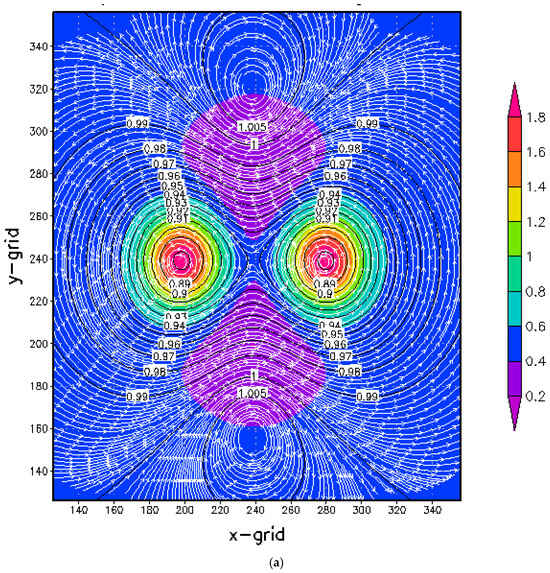
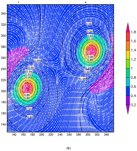
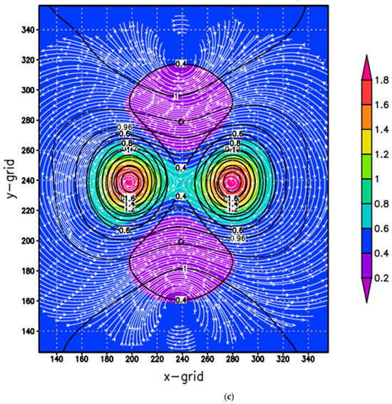
Figure 5.
(a) Potential vorticity (colormap), height (black), and stream function (white) at t = 0 for Case B. (b) Potential vorticity (colormap), height (black), and stream function (white) from forward integration at t = 40 for Case B. (c) Potential vorticity (colormap) and stream function (white) from backward integration at t = 0 using forward integration at t = 40 as initial condition. Black contour shows initial condition of forward integration at t = 0.
5. Discussion
Traditionally, turburlences occur when the Reynolds number (UL/ν) is greater than a threshold. The Reynolds number is infinity in inviscid fluid (i.e., viscosity ν → 0 in this 2D flow), and the simulated flows, instead of becoming chaotic turbulences, are well organized because of fast rotaton. In Section 2, we also demonstrated that the model can be applied to vortex merging for both forward and backward integrations by changing the sign of dt. The simulations from backward integration are the image of forward integration, and vice versa. It also indicates when t > 120 in forward integration or t < −120 in backward integration, the merged system becomes very stable and the pattern changes little as time increases in both integrations. The fast rotation enhances the stability of the 2D system in vortex merger, which contributes little to inverse energy flux [46,47]. It is also noted that laminar co-rotating vortices were obseved in both experiemnts and model simulations [26]. Hence, after |t| > 60, the model fails to retrive the initial condtion at t = 0 from either forward or backward integration. The time scale to retrieve the initial condition is shorter than that of inverse integration of soliton Rossby waves because the pattern changes drastically in vortex merger but the pattern remains the same in soliton waves. Discrepancy between forward and backward time-step calcualtions prevents the simulations from retrieving the initial condition.
A simple numerical scheme of 1D advection equation can be written as follows:
In forward integration,
but in back integration,
calculated from (32) is different from (33). Hence, if you integrate forward from n to n + 1 time-step, then, integrated backward from n + 1 to n time-step, the result is usually different from the original value, unless implicit schemes are used in (32) and (33). It is noted that implicit scheme was applied to the backward integration of diffusion equation; therefore, it was able to retrieve the initial species [19]. The discrepancy depends on the property of equations and accuracy of the numerical scheme. Hence, after long integrations, the reverse integrations in Section 4 depart from the initial values (t = 0) of forward integration. On the other hand, when backward and forward integrations use the same initial condition, the backward integration at −t is the image of the forward integration at t, as discussed in Section 3. In addition to using the implicit scheme, we can replace the fourth order advection scheme by semi-Lagrangian schemes [51,52] to reduce the phase errors of the short waves [53]. Poincare [54,55] discovered that a minor change in one state of a deterministic nonlinear system can result in significant differences in a later state. Lorenz [56] rediscovered the chaotic behavior and tractors of a nonlinear system. It is also noted that, after a long integration in both forward and backward integrations, the system approaches stable attractors and cannot return to the initial condition at t = 0.
6. Summary
The numerical model [21] can be a useful tool to study highly nonlinear shallow water equations because it does not encounter the constrains/difficulty which may occur in asymptotic analysis or Bäcklund transform. Using the same initial condition, the model simulations from backward integration are the image of forward integration. After long integrations, vortices merge and form a stable core surrounded by long filaments. The total energy and total enstrophy remain near constant with time in both forward and backward integrations. Meanwhile, the energy spectra move toward longwave but do not grow with time. The effect of fast rotation makes the 2D flow more stable than the 3D flow. The system remains well orgainized instead of caotic, where even the pattern changes drastically during the merge of two vortices. The effect of fast rotation also supresses inverse and direct energy cascades in an inviscid fluid. The slope of the enegy inverse cascade is around −2, which is close to the previous studies [48,49]. The slope of energy on shortwaves is much steeper than −3, propsoed by Kraichnan [40], which is also due to no dissipation (ν = 0) and the effect of fast roation.
The system changes drastically during vortices merging. After the integer time t > 60 in forward integration (or t < −60 in backward integration), the system cannot retrive its initial condition from either integration because the change within a time-step of forward intgration is not exactly the same as backward integration, as dicussed. The implicit schemes and semi-Lagrangian schemes may increase computing accuracy and extend the retrival time in backward integration.
Funding
This research received no external funding.
Institutional Review Board Statement
Not applicable.
Informed Consent Statement
Not applicable.
Data Availability Statement
The original contributions presented in this study are included in the article. Further inquiries can be directed to the corresponding author.
Acknowledgments
The author is grateful to reviewers for their useful comments. He also thanks P. Lin and C. Huang for providing computing facility and N. Lin and M. Yen at NCU and Taiwan National Science and Technology Council for their support when the author worked on this research.
Conflicts of Interest
The author declares no conflict of interest.
References
- Boussinesq, J. Essai sur la Theorie des Eaux Courantes. Memoires Presentes par Divers Savants a L’academie des Sciences de L’institut National de France, 13th ed.; Imprimerie Nationale: Paris, France, 1877; pp. 1–680. [Google Scholar]
- Wikipedia Korteweg-de Vries Equation. Available online: https://en.wikipedia.org/wiki/Korteweg%E2%80%93De_Vries_equation (accessed on 20 March 2025).
- Korteweg, D.J.; de Vries, G. On the change of form of long waves advancing in a rectangular canal, and on a new type of long stationary waves. London Edinburgh Dublin Philos. Mag. J. Sci. 1895, 39, 422–443. [Google Scholar]
- Konno, K.; Wadati, M. Simple derivation of Backlund Transformation from Riccati form of inverse method. Prog. Theor. Phys. 1975, 53, 1652–1656. [Google Scholar]
- Griffiths, G.W. Ba¨cklund Transformation. Phys. Rev. Lett. 2012, 31, 1386. Available online: https://www.researchgate.net/profile/Graham-Griffiths2/publication/269408982_Backlund_Transformation/links/58b942ac45851591c5d811d3/Baecklund-Transformation.pdf (accessed on 1 January 2024).
- Gadioux, R. Using Ba¨cklund Transformations to Find Soliton Solutions. 2022. Available online: https://www.universityofgalway.ie/media/collegeofscience/schools/schoolofmathematics/files/Romain-Gadioux---Using-B%C3%A4cklund-Transformations-to-Find-Soliton-Solutions.pdf (accessed on 12 December 2024).
- Gao, X.-Y. Symbolic Computation on a (2 + 1)-Dimensional generalized nonlinear evolution system in fluid dynamics, Plasma Physics, Nonlinear Optics and Quantum Mechanics. Qual. Theory Dyn. Syst. 2024, 23, 202. [Google Scholar] [CrossRef]
- Gao, X.Y. Hetero-Bäcklund transformation, bilinear forms and multi-solitons for a (2+1)-dimensional generalized modified dispersive water-wave system for the shallow water. Chin. J. Phys. 2024, 92, 1233–1239. [Google Scholar] [CrossRef]
- Hu, X.-R.; Chen, Y. Bäcklund transformations and explicit solutions of (2+1)-dimensional barotropic and Quasi-Geostrophic Potential Vorticity equation. Commun. Theor. Phys. 2010, 53, 803–808. [Google Scholar]
- Kuo, H.L.; Platzman, G.W. An Investigation of the Nonlinear Solution of the Rayleigh Convection Problem by Means of Characteristic Functions; Department of Meteorology, University of Chicago: Chicago, IL, USA, 1960; p. 76. [Google Scholar]
- Segur, H. Lecture 5: Waves in Shallow Water, Part I: The Theory. 2009. Available online: https://gfd.whoi.edu/wp-content/uploads/sites/18/2018/03/lecture5-harvey_136544.pdf (accessed on 20 January 2025).
- Boyd, J.P. Equatorial solitary waves. Part-1: Rossby solitons. J. Phys. Ocean. 1980, 10, 1699–1717. [Google Scholar]
- Boyd, J.P. Equatorial solitary waves. Part 3: Westward-traveling motions. J. Phys. Ocean. 1985, 15, 46–54. [Google Scholar]
- Liao, S. An optimal homotopy-analysis approach for strongly nonlinear differential equations. Commun. Nonlinear Sci. Numer. Simulat. 2009, 15, 2003–2016. [Google Scholar] [CrossRef]
- Fourier, J.B.J. Theorie Analytique de la Chaleur; Didot: Paris, France, 1822; pp. 499–508. [Google Scholar]
- Keller, J.J. Inverse Euler equation. Z. Angew. Math. Phys. 1966, 49, 363–383. [Google Scholar]
- Kalnay, E.; Park, S.K.; Pu, Z.-X.; Gao, J. Application of the Quasi-Inverse Method to Data Assimilation. Mon. Wea. Rev. 2000, 128, 864–875. [Google Scholar] [CrossRef]
- Van Leeuwen, T.; Brune, C. 10 Lectures on Inverse Problems and Imaging. 2025. Available online: https://tristanvanleeuwen.github.io/IP_and_Im_Lectures/intro.html (accessed on 10 January 2025).
- Sun, W.Y.; Sun, O.M. Backward Integration of Diffusion Equation. Aerosol Air Qual. Res. 2017, 17, 278–289. [Google Scholar] [CrossRef]
- Sun, W.Y. Backward Integration of Nonlinear Shallow Water Model: Part I: Solitary Rossby Waves. Atmosphere 2024, 15, 1161. [Google Scholar] [CrossRef]
- Sun, W.Y. Instability in leapfrog and forward–backward schemes: Part II: Numerical simulations of dam break. Comput. Fluids 2011, 45, 70–76. [Google Scholar] [CrossRef][Green Version]
- Melander, M.V.; Zabusky, N.J.; McWilliams, J.C. Symmetric vortex merger in two dimensions: Causes and conditions. J. Fluid. Mech. 1988, 195, 303–340. [Google Scholar] [CrossRef]
- Waugh, D.W. The efficiency of symmetric vortex merger. Phys. Fluid Dyn. 1992, 4, 1745–1758. [Google Scholar] [CrossRef]
- Oh, T.J. The Development and Testing of Characteristic-based Semi-Lagrangian Two-Dimensional Shallow Water Equations Model. Ph.D. Thesis, Purdue University, West Lafayette, IN, USA, 2020. Available online: https://docs.lib.purdue.edu/dissertations/AAI3278686/ (accessed on 20 March 2025).
- Huang, S.; Xiang, J.; Du, H.; Cao, X. Inverse problems in atmospheric science and their application. J. Phys. Conf. Ser. 2005, 12, 45–57. [Google Scholar] [CrossRef]
- Meunier, P.; Le Dizès, S.; Leweke, T. Physics of vortex merging. Comptes Rendus Phys. 2005, 6, 431–450. [Google Scholar] [CrossRef]
- Sun, W.Y.; Oh, T.J. Vortex merger in shallow water model. Asia-Pacific J. Atmos. Sciences 2022, 58, 533–547. [Google Scholar] [CrossRef]
- Duponcheel, M.; Orlandi, P.; Winckelmans, G. Time-reversibility of the Euler equations as a benchmark for energy conserving schemes. J. Comput. Phys. 2008, 19, 8736–8752. [Google Scholar] [CrossRef]
- Eckhardt, B.; Hascoet, E. Breaking time reversal symmetry by viscous dephasing. Phys. Rev. E 2005, 72, 037301. [Google Scholar]
- Fang, L.; Bos, W.J.T.; Liang, S.; Bertoglio, J.-P.; Shao, L. Time reversibility of Navier-Stokes turbulence and its implication for subgrid scale models. J. Turbul. 2012, 13, 639777. [Google Scholar]
- Sun, W.Y. The Vortex Moving toward Taiwan and the influence of the Central Mountain Range. Geosci. Lett. 2016, 3, 21. [Google Scholar] [CrossRef]
- Sun, W.Y. Challenges and Progress in Computational Geophysical Fluid Dynamics in Recent Decades. Atmosphere 2023, 14, 1324. [Google Scholar] [CrossRef]
- Miller, A. MODULE Fast Fourier. 2005. Available online: https://jblevins.org/mirror/amiller/fft.f90 (accessed on 4 October 2024).
- Vallis, G.K. Fundamentals and Large Scale Circulation. In Atmospheric and Oceanic Fluid Dynamics; Cambridge University Press: Cambridge, UK, 2005; p. 774. [Google Scholar]
- Kolmogorov, A.N. The local structure of turbulence in incompressible viscous fluid for very large Reynolds numbers. Dokl. Acad. Sci. USSR 1941, 30, 299–303. [Google Scholar]
- Obukhov, A.M. Energy distribution in the spectrum of turbulent flow. Izv. Akad. Nauk. SSR Ser. Geogr. Geofiz. 1941, 5, 453–466. [Google Scholar]
- Batchelor, G.K. The theory of homogeneous turbulence. In Cambridge Monographs on Mechanics and Applied Mathematics; Cambridge University Press: Cambridge, UK, 1953; p. 197. [Google Scholar]
- Fjørtoft, R. On the changes in the spectral distribution of kinetic energy for two dimensional nondivergent flow. Tellus 1953, 5, 225–230. [Google Scholar]
- Batchelor, G.K. Computation of the energy spectrum in homogeneous two dimensional turbulence. Phys. Fluids Suppl. 1969, 12, 233–239. [Google Scholar]
- Kraichnan, R. Inertial ranges in two-dimensional turbulence. Phys. Fluids 1967, 10, 1417–1423. [Google Scholar]
- Kraichnan, R.; Montgomery, D. Two-dimensional turbulence. Rep. Prog. Phys. 1980, 43, 547–619. [Google Scholar]
- Nastrom, G.; Gage, K.; Jasperson, W. Kinetic energy spectrum of large-and mesoscale atmospheric processes. Nature 1984, 310, 36–38. [Google Scholar] [CrossRef]
- Kraichnan, R. Inertial-range transfer in two- and three-dimensional turbulence. J. Fluid Mech. 1971, 47, 525–535. [Google Scholar] [CrossRef]
- Deusebio, E.; Boffetta, G.; Lindborg, E.; Musacchio, S. Dimensional transition in rotating turbulence. Phys. Rev. E 2014, 90, 023005. [Google Scholar] [CrossRef]
- Taylor, G.I. Experiments with rotating fluids. Proc. Roy. Soc. Lond. A 1921, 100, 114–121. [Google Scholar]
- Xiao, Z.; Wang, X.; Chen, S.; Eyink, G. Physical mechanism of the inverse energy cascade of two-dimensional turbulence: A numerical investigation. J. Fluid Mech. 2009, 619, 1–44. [Google Scholar]
- Boffetta, G.; Ecke, R.E. Two-Dimensional Turbulence Annu. Rev. Fluid Mech. 2012, 44, 427–451. [Google Scholar]
- Morize, C.; Moisy, F. Energy decay of rotating turbulence with confinement effects. Phys. Fluids 2006, 18, 065107. [Google Scholar]
- Zhou, Y. A phenomenological treatment of rotating turbulence. Phys. Fluids 1995, 7, 2092. [Google Scholar]
- Pouquet, A.; Sen, A.; Rosenberg, D.; Mininni, P.D.; Baerenzung, J. Inverse cascades in turbulence and the case of rotating flows. Phys. Scr. 2013, T155, 014032. [Google Scholar] [CrossRef]
- Sun, W.Y.; Yeh, K.S.; Sun, R.Y. A simple Semi-Lagrangian Scheme for advection equation. Q. J. R. Meteorol. Soc. 1996, 122, 1211–1226. [Google Scholar]
- Sun, W.Y. An efficient forward semi-Lagrangian model. Terr. Atmos. Ocean. Sci. 2024, 35, 2. [Google Scholar] [CrossRef]
- Sun, W.Y. Numerical experiments for advection equation. J. Comput. Phys. 1993, 108, 264–271. [Google Scholar] [CrossRef]
- Poincaré, H. Sur les Fonctions Fuchsiennes. Comptes Rendus Hebd. L’académie Sci. Paris 1882, 94, 1166–1167. [Google Scholar]
- Poincaré, H. Solutions Periodiques, Non-Existence des Integrales Uniformes, Solutions Asymptotiques; Gauthier-Villars: Paris, France, 1892; Volume 1. (In French) [Google Scholar]
- Lorenz, E.N. Deterministic nonperiodic flow. J. Atmos. Sci. 1963, 20, 130–141. [Google Scholar] [CrossRef]


Disclaimer/Publisher’s Note: The statements, opinions and data contained in all publications are solely those of the individual author(s) and contributor(s) and not of MDPI and/or the editor(s). MDPI and/or the editor(s) disclaim responsibility for any injury to people or property resulting from any ideas, methods, instructions or products referred to in the content. |
© 2025 by the author. Licensee MDPI, Basel, Switzerland. This article is an open access article distributed under the terms and conditions of the Creative Commons Attribution (CC BY) license (https://creativecommons.org/licenses/by/4.0/).