The Positive Effects of Linked Control Policy for Vessels Passing Through Locks on Air Quality—A Case Study of Yichang, China

Abstract

During the waiting period before passing through locks, inland vessels typically rely on diesel generators to power their onboard equipment, which leads to air pollution and poses more direct threats to the surrounding residents and ecological environment. To assess the extent to which green and efficient lock passage strategies can reduce air pollution, this study takes the Linked Control Policy for Vessels Passing Through Locks released by the Three Gorges Navigation Authority in China in December 2017 as the research object. It collected air quality monitoring data for six years before and after the policy implementation (2014–2020) and used a Regression Discontinuity model (RD model) to analyze the policy’s effect. The results show that compared to 2014, the average concentration of SO₂ in the air decreased by 67% in 2020, along with NO₂ decreasing by 32%, PM_2.5 by 42%, PM₁₀ by 46%, and the AQI (Air Quality Index) by 27%. The robustness test of the RD model also confirmed the causal relationship between the policy implementation and the improvement in air quality. This research is the first to systematically disclose the environmental benefits of the “soft” management policy of optimizing the lock passage process, uncovering the positive influence of active ship lock passage policy on air quality, and providing a scientific basis for promoting the implementation of policies related to lock management.

1. Introduction

Ship exhaust emissions have brought severe hazards to the environment and human health. Sulfur oxides, nitrogen oxides, and particulate matter in the exhaust are the primary harmful substances [1,2]. Among them, sulfur oxides, when combined with water vapor, tend to form acid rain, corroding buildings and undermining the ecological environment [3]; nitrogen oxides not only exacerbate photochemical smog but also harm the human respiratory system, increasing the risk of respiratory diseases [4]. Particulate matter can penetrate deep into the lungs, triggering cardiopulmonary diseases, and even cause cancer [5,6].

At present, people’s concern about the hazards of ship emissions mainly focuses on ocean-going vessels because of their large fuel consumption and low fuel quality, which leads to more severe air pollution [7,8,9]. However, research and analysis on the influence of inland waterway vessel emissions are relatively scarce. Nevertheless, hinterland waterways are usually close to densely populated areas and water source protection zones, and exhaust pollution has a more direct and significant impact on the health of coastal residents and the environmental quality [10]. On the other hand, the navigation conditions of inland waterway vessels are restricted, such as narrow waterways and complex water flows, which may result in different emission characteristics compared to seagoing vessels, increasing the complexity and challenges of emission control. Therefore, in recent years, some scholars have begun to conduct research and analyses on the influence of inland waterway vessel emissions [11,12].

Among the management aspects of inland waterway vessels, the waiting issue during lock passage scheduling is a complex and urgent challenge to be addressed [13]. Due to the limited capacity of the locks, numerous vessels need to queue in a certain sequence to pass through, often resulting in lengthy waiting times [14]. During the waiting period, vessels not only consume additional fuel to maintain their position and status but also increase air pollutant emissions, exerting adverse effects on the environment and the nearby residents. Moreover, prolonged waiting may also induce fatigue and anxiety among vessel operators, raising the risk of safety accidents. Hence, optimizing the lock passage scheduling mechanism to reduce waiting times is of great significance for enhancing navigation efficiency and ensuring safety and environmental protection.

Minimizing fuel emissions and maximizing navigation efficiency are generally the objectives of green lock scheduling research [15,16]. The scheduling process involves optimizing the lock timetable, vessel entry times, and vessel positions within the lock chamber, which is a nonlinear programming problem [17]. Simultaneously, the lock passage problem involves the scheduling of multiple vessels and requires overall consideration of the optimization strategies and hierarchical adjustments [18]. Additionally, lock scheduling also has an impact on the operation of the surrounding docks, making it a problem that requires coordinated scheduling optimization, further intensifying the research challenges of lock scheduling [19]. Reducing the negative impact of lock passage on shipping requires not only the improvement of infrastructure in inland waterways but also a comprehensive consideration of how to optimize the scheduling problem to enhance the efficiency of vessel lock passage and reduce exhaust emissions [20,21].

Therefore, rational lock passage scheduling can effectively reduce vessel waiting times and lower fuel consumption and pollutant emissions, thereby alleviating the pressure on the environment [22]. Simultaneously, it can ensure the rational utilization of waterway resources, avoid congestion and delays, and improve the operational efficiency of the entire shipping system. Previous studies have mainly focused on the optimization of scheduling strategies; for example, Golak presented a mathematical programming formulation of the speed optimization problem [23], which aims to minimize the aggregated fuel consumption on an inland waterway network. Smith constructed a discrete-event simulation model to investigate the impact of alternative decision rules and infrastructural improvements to relieve traffic congestion in a section of the Upper Mississippi River (UMR) navigation system [24]. Segovia formulated the vessel passage scheduling problem as a mixed-integer programming problem to ensure efficient inland waterway transport, considering the operation of sequential movable bridges required for vessel passage [25]. Pang constructed an optimization model for joint scheduling of a double-line ship lock based on nonlinear goal programming, aiming to improve ship lock capacity, assuming a relatively stable number of ships waiting for the lock [26]. But the assessment of the effectiveness of these strategies has been rarely involved, especially the positive effects on the environment, such as air quality. This project takes the Linked Control Policy for Vessels Passing Through Locks of the Three Gorges Navigation Authority as the research object. Based on the Regression Discontinuity model (RD model), it analyzes the positive effect of the policy on enhancing the air quality of Yichang City. Since a symmetrical time window can offer a more balanced data distribution and be conducive to analysis, an excessive time gap before and after the breakpoint might be influenced by other factors, resulting in estimation bias. This study merely collects the air quality data of Yichang City within three years before and after the implementation of the policy and assesses the positive influence of the ship lock passage policy on reducing the exhaust pollution of inland waterway vessels from the perspective of green shipping.

2. Materials and Methods

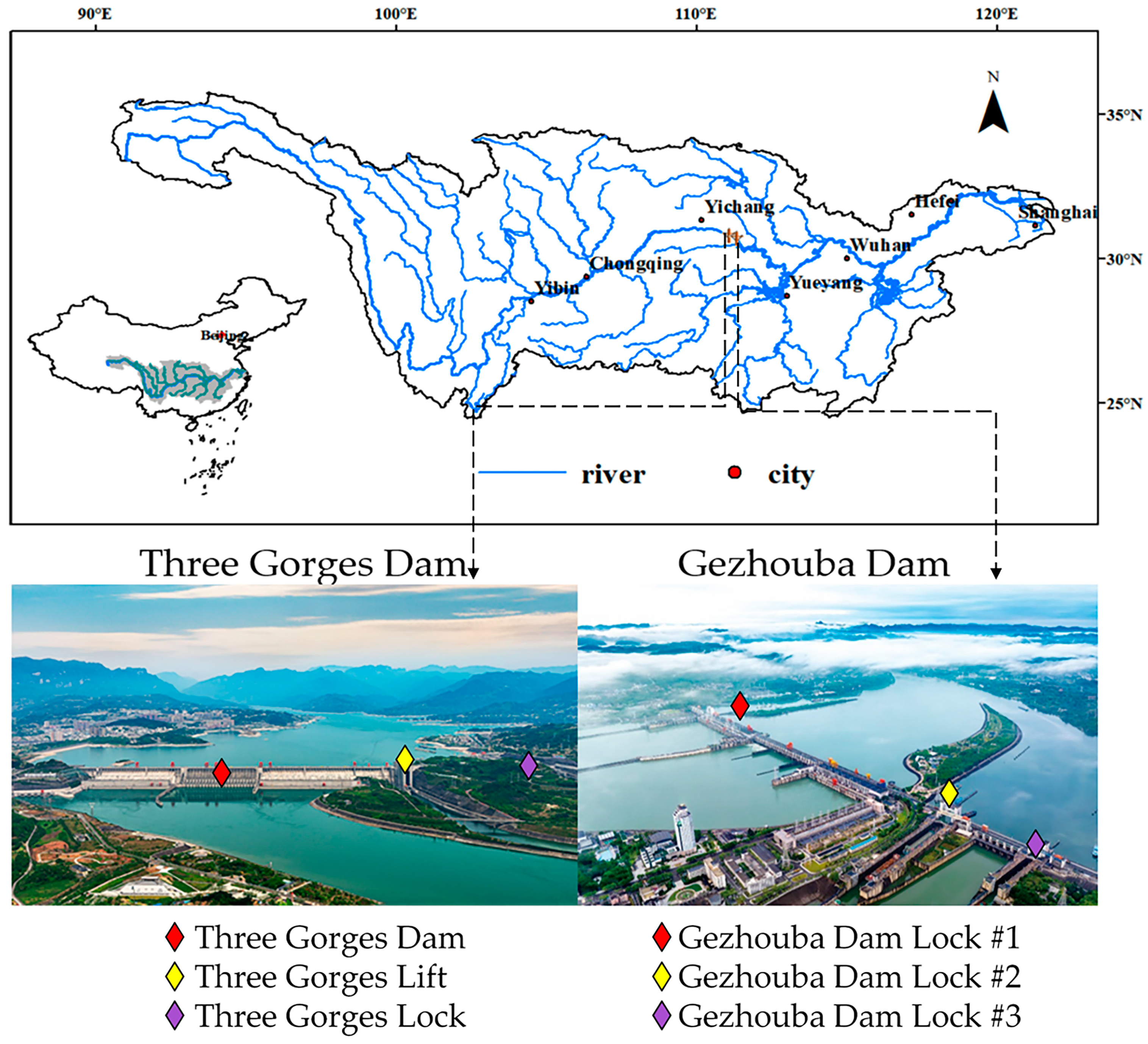
2.1. Location

The location of this study is Yichang City, Hubei Province, China, which is situated at the demarcation point between the upper and middle reaches of the Yangtze River. The terrain is relatively complex, with a significant disparity in elevation, and has a subtropical monsoon humid climate, covering an area of 21,000 square kilometers. As of the end of 2023, the resident population of Yichang City was 3.924 million [27]. Two major dams, the Three Gorges Dam and the Gezhouba Dam, are present within Yichang City, as shown in Figure 1.

The statistical data from the Three Gorges Navigation Authority indicate that in 2024, the throughput of the Three Gorges Hub amounted to 159 million tons. The Three Gorges Ship Lock operated more than 10,000 times, with a throughput of 154 million tons; the Three Gorges Ship Lift operated over 4700 times, handling 5.03 million tons [28]. It can be observed from Figure 1 that both of these dams are close to populated areas, and the exhaust emissions from ships directly impact the overall air quality of Yichang City. This study selects the Three Gorges Ship Lock area as the research object, primarily due to the following considerations: Firstly, the Three Gorges Ship Lock is one of the world’s busiest inland ship locks and serves as a critical hub on the Yangtze River Golden Waterway. It connects China’s eastern coastal economic zone with its central and western regions, handling a substantial proportion of the river’s freight and passenger traffic. Consequently, ship activities in this region significantly influence atmospheric pollutant emissions (such as SO₂, NO₂, PM_2.5, and PM₁₀), making the research results invaluable for understanding pollution characteristics and control strategies in inland shipping. Secondly, air pollution in the Three Gorges Ship Lock area is particularly severe, largely attributed to ship emissions. Ships must wait for extended periods before entering the lock and require significant power usage during passage, leading to concentrated emissions. As a typical operating environment for inland ship locks, studying its emission characteristics and pollution impacts provides crucial references for other inland waterways. Additionally, this area is ideal for assessing policy interventions, allowing for precise quantification of policy effects. Unlike seaports or open waters, the Three Gorges Ship Lock operates as a closed, high-density traffic node with relatively fixed ship activity patterns, facilitating easier identification of pollutant emission characteristics. Furthermore, the ship lock linkage control policy that was officially implemented in December 2017 provided a natural policy breakpoint for this study, enabling the RD model to identify the impact of this policy on air quality more accurately. Therefore, choosing the Three Gorges Ship Lock as the research area can evaluate the actual effect of the policy more reliably on the basis of controlling external interference factors.

2.2. Policy

The passage of ships through locks is mainly conducted by queuing and waiting. Vessels frequently concentrate near the lock gates, causing prolonged congestion. This pattern increases the idle running time of ships, resulting in higher fuel consumption and exhaust emissions. Meanwhile, it has an adverse impact on the air quality of the surrounding residents [29,30]. On 27 December 2017, the Three Gorges Navigation Authority promulgated the “Plan for Coordinated Control and Transportation Organization of Ships Passing Through the Dam on the Main Line of the Yangtze River” to mitigate the negative influence of passing ships on the air quality of Yichang City [31]. The policy is referred to hereinafter as the ship lock passage policy. The implementation scheme of this policy can be generalized as follows:

Water area division: According to the distance of vessels from the Three Gorges Dam, the main channel of the Yangtze River is divided into five zones—core water area, near-dam water area, control water area, dispatch water area, and remote water area—to manage the passage order of vessels in a hierarchical manner. The core water area is the last waiting area before passing through the dam. All vessels entering this area must strictly follow the dispatch instructions to execute the dam passage plan, ensuring the smoothness of the waterway and reducing unnecessary emissions. The near-dam water area serves as a buffer zone where some vessels can wait for passage, reducing the traffic pressure in the core water area. The control water area covers a larger waiting area and allows some vessels to enter the queuing sequence in advance, reducing traffic congestion in case of emergencies. The dispatch water area is mainly used for the management of vessels far from the dam area, ensuring the smooth flow of traffic. The remote water area covers the far end of the main channel of the Yangtze River and is used for early control of vessels that have not yet entered the main queuing sequence to prevent congestion caused by a large number of vessels concentrating in the near-dam area.

Dam passage declaration system: Vessels passing through the Three Gorges Dam on the Yangtze River must submit remote dam passage applications through the Yangtze River Three Gorges Waterborne GPS Positioning Comprehensive Application System to achieve real-time monitoring and management of vessel information. For vessels that do not have the conditions for GPS declaration, they need to submit written dam passage applications to the maritime authority and be approved before being entered into the system. All vessels that have passed the declaration must keep their GPS and AIS devices on to ensure real-time tracking of their positions and avoid affecting the execution of the dam passage plan due to loss of positioning.

Vessel sequencing management: The sequencing of vessels passing through the dam is confirmed based on the time they pass through the Shishou Yangtze River Bridge (upstream) or the Yunyang Yangtze River Bridge (downstream) to ensure fairness and passage efficiency. To enhance the orderliness of traffic management, the policy stipulates that vessels are classified and sequenced by type, including hazardous cargo vessels, container ships, and vehicle carriers, among others. Special mission vessels, long-distance passenger ships, vessels carrying fresh and live cargo, and those transporting key and urgent materials are given priority passage to ensure the smooth flow of emergency supplies and special shipping needs.

Rolling plan formulation: This policy implements a rolling plan management model to dynamically adjust vessel passage schedules and enhance the flexibility of shipping dispatch. The Three Gorges Navigation Command Center publishes a 24 h daily operation plan at 3 pm each day to ensure efficient short-term dispatch execution. Additionally, it releases a rolling pre-plan at 9 am daily to notify vessels already in the queue for passage, allowing them to optimize their sailing times, minimize unnecessary waiting, and consequently reduce fuel consumption and pollutant emissions.

The waiting zone system: It stipulates that vessels awaiting passage must comply with the principles of “total volume control, segmented management, staged waiting, and orderly release” to mitigate traffic congestion and optimize the management of waiting areas. The core waters impose strict entry restrictions, permitting only vessels listed in the 1–2 day rolling pre-plan to wait there, thereby alleviating pressure on the waterway. Vessels listed in the 3-day rolling pre-plan may wait in the near-dam waters but are required to enter the core waters within 24 h to minimize uncertainty in berthing times. Vessels listed in the 4-day or later rolling pre-plans can wait in the control waters to reduce safety risks associated with frequent repositioning. Additionally, dispatching waters accommodates vessels waiting for longer-term plans, preventing a surge of vessels into the near-dam area. Priority vessels are allowed direct access to the core waters to ensure the smooth execution of critical transportation tasks.

Information Disclosure Mechanism: To enhance the transparency of policy implementation, the government website (www.sxthj.org.cn, accessed on 28 February 2025.) publishes daily the over-dam operation plans, rolling pre-plans, priority vessel lists, and the number of vessels waiting at each water area, enabling vessel operators to obtain the latest passage information. Meanwhile, the policy requires that the investigation and handling of vessels in violation be promptly disclosed to ensure the traceability of violations and strengthen the policy’s binding force. Additionally, the policy has established a dedicated hotline for vessel operators to report and supervise violations, forming a comprehensive information feedback mechanism to further improve the policy’s enforcement and fairness.

In summary, the policy improves ship traffic efficiency and reduces congestion and waiting time through fine water division, an intelligent declaration system, hierarchical ranking management, dynamic rolling scheduling, a reasonable lock waiting mechanism, and an information disclosure system. While ensuring shipping safety, it also reduces the impact of ship emissions on air quality along the river. It provides a management model for other inland shipping hubs.

2.3. Data

This research gathered information on the concentrations of the air pollutants SO₂, NO₂, and Particulate Matter 2.5 (PM_2.5), and Particulate Matter 10 (PM₁₀), as well as the values of the AQI (Air Quality Index) from the online monitoring and analysis platform for air quality in China at https://www.aqistudy.cn (accessed on 17 March 2025). The calculation approach of AQI employed the concentration limits stipulated in the “Ambient Air Quality Standards” GB 3095-2012 formulated by the Ministry of Ecology and Environment of the People’s Republic of China [32]. Furthermore, we also collected data on the industrial dust emissions (hereinafter referred to as IDE; unit: tons), industrial SO₂ emissions (hereinafter referred to as ISE; unit: tons), and industrial wastewater emissions (hereinafter referred to as IWE; unit: ten thousand tons) in Yichang City during the same period. The data originated from the Hubei Provincial Bureau of Statistics at https://tjj.hubei.gov.cn/ (last access was on 17 March 2025).

Annually, from March to November, the concentrations of SO₂, NO₂, PM_2.5, and PM₁₀ and the AQI values are relatively low, while from December to February of the subsequent year, the concentrations of all these pollutants are generally higher. Through preliminary data statistics, it can be discerned that the concentrations of particulate matter from March to November are typically lower than those from December to February of the following year. For example, the average concentration of SO₂ from March to November is 10 µg/m³, while that from December to February of the subsequent year is 18 µg/m³. The average concentrations of other particulate matter exhibit the same pattern as SO₂, with higher average concentrations in winter compared to other seasons. The primary reason for this phenomenon is that the temperature inversion in winter precludes pollutants from ascending to higher altitudes, causing them to accumulate near the ground and deteriorating air quality. Additionally, the augmented demand for heating in winter, particularly the utilization of coal and gas, leads to increased emissions of pollutants such as sulfur dioxide, nitrogen oxides, and particulate matter. The low wind speed and lower air humidity also render it difficult for pollutants to disperse or settle, further exacerbating pollution levels. Coupled with traffic emissions and stable weather conditions, all these factors jointly contribute to higher concentrations of pollutants in winter compared to other seasons, resulting in poorer air quality. To circumvent the influence of typically poorer air quality in winter on the RD model’s discontinuity regression calculation, this study divided the data into three groups and employed the RD model for computation. The first group encompassed all the data from 2014 to 2020 for calculation. The second group solely considered the calculation data from the winter months (December to February of the following year), and the third group exclusively included the data from the spring, summer, and autumn months (March to November), as shown in

Table 1. Descriptive statistics of the variables.

Groups	Variable	Obs.	Mean.	Std. Dev.	Min.	Max.
1	SO2	2187	12	9	3	92
	NO2		32	11	8	83
	PM2.5		56	43	3	318
	PM10		84	52	8	407
	AQI		87	48	21	368
	IDE		44	19	21	82
	ISE		72	59	16	199
	IWE		26	12	16	50
2	SO2	538	18	14	5	92
	NO2		38	13	8	83
	PM2.5		105	50	10	318
	PM10		131	63	16	407
	AQI		138	60	26	368
	IDE		46	19	21	82
	ISE		72	59	16	199
	IWE		27	13	16	50
3	SO2	1649	10	5	3	56
	NO2		29	9	12	64
	PM2.5		40	25	3	206
	PM10		68	35	8	286
	AQI		71	28	21	256
	IDE		43	19	21	82
	ISE		72	59	25	199
	IWE		26	12	16	50

Obs. represents the number of samples; Mean, Min, Max, and Std. dev. represent the average value, minimum value, maximum value, and standard deviation of SO₂, NO₂, PM_2.5, PM₁₀, and AQI concentrations, respectively. IDE, ISE, and IWE, respectively, refer to industrial dust emissions, industrial SO₂ emissions, and industrial wastewater emissions. The concentration units of all pollutants are µg/m³, the units of IDE and ISE are tons, the unit of IWE is ten thousand tons, and AQI has no unit. This study divided the data into three groups and employed the RD model for computation. The first group encompassed all the data from 2014 to 2020 for calculation. The second group solely considered the calculation data from the winter months (December to February of the following year), and the third group exclusively included the data from the spring, summer, and autumn months (March to November). Lastly, 1, 2, and 3 respectively refer to the first group, the second group, and the third group.

.

2.4. Model

The RD model is a quasi-experimental approach employed for assessing the efficacy of policies or intervention measures [33]. Its core notion is to divide the sample into treatment and control groups by leveraging a distinct cut-off point (such as time, score, etc.) [34].

Supposing that individual characteristics are similar in the vicinity of the breakpoints, the effect of policy schemes can be estimated by comparing the outcome differences on both sides of the breakpoint. In this research, the ship dispatching plan in Yichang City was implemented at a specific time. Hence, this time point can be utilized as a demarcation line to construct an RD model for analyzing the influence of the policy on air quality. The advantage of this approach lies in that it can simulate causal inference in a non-random experimental setting. Comparing the alterations in air quality before and after policy implementation, it reduces the interference from other external factors and guarantees the reliability of the estimation results. To ensure the robustness of the model, additional stability tests are typically conducted to verify whether the fundamental characteristics of the samples on both sides of the breakpoint are similar prior to the policy implementation. Meanwhile, appropriate bandwidth selection is adopted to ensure that the analysis focuses on the crucial data around the time when the policy becomes effective. Through these mechanisms, the RD model is capable of precisely assessing the actual impact of policies, making it a frequently employed analytical tool in domains such as environmental governance measures and social policy interventions.

In this study, the fundamental principle of the method is presented as Formula (1).

$$Y_t={\alpha }_0+r{D}_t+{\alpha }_{1}f\left(x_t\right)+{\alpha }_2{D}_{t}f\left(x_t\right)+\phi Z_t+{\mu }_t$$

(1)

Herein, Y_t denotes the average mass concentrations of SO₂, NO₂, PM_2.5, and PM₁₀, along with the AQI value measured at moment t. α₀ represents the individual fixed effect, which is an unobservable variable influencing Y_t, but remains invariant with time at the individual level. r indicates the coefficient of the treatment variable D_t, reflecting the treatment effect of the policy. When t < 0, it implies that the policy has not been implemented, and at this point, D_t = 0. When t ≥ 0, it suggests that the policy has been implemented, and at this juncture, D_t = 1. If r is statistically significant, it suggests that the implementation of the policy has a significant correlation with the levels of SO₂, NO₂, PM_2.5, PM₁₀, and AQI in Yichang City; if r is not significant, it indicates that the implementation of the policy has no significant influence on the alterations in air quality. f(x_t) is the polynomial trend term function of time t, and α₁ is its estimated coefficient. D_tf(x_t) represents the interaction term between the treatment variable and the time trend term, facilitating a better understanding of their combined effect on the outcome variable, and α₂ is the estimated coefficient of D_tf(x_t). The relevant control variable Z_t encompasses industrial smoke and dust emissions, industrial sulfur dioxide emissions, and industrial wastewater emissions. φ represents its effect coefficient. μ_t represents the error term, accounting for unknown contributing factors.

The core of the RD model lies in leveraging the policy implementation time point as a breakpoint to construct a pre- and post-comparison for evaluating the policy effect. The time trend term f(x_t), acting as a function to describe the long-term variations in pollutant concentrations, has appropriate polynomial orders selected for different pollutants in this research. Specifically, a ninth-order polynomial (order = 9) is adopted for SO₂, NO₂, PM_2.5, and PM₁₀, while an eighth-order polynomial (order = 8) is used for AQI. The selection of polynomials is based on the Akaike Information Criterion (AIC) and the Bayesian Information Criterion (BIC) to ensure the optimal fitting of the model and simultaneously avoid overfitting. Regarding data processing, the time variable x_t is initially set with December 2017 as the reference point, and the policy treatment variable D_t is calculated for each time point. Subsequently, the pollutant concentration data are regarded as the dependent variable, while the time trend term f(x_t), the policy variable D_t, and their interaction term D_tf(x_t) are utilized as independent variables. Ordinary Least Squares (OLS) regression is employed to estimate the actual influence of the policy. Additionally, to mitigate the interference of external factors, industrial dust emissions (IDE), industrial SO₂ emissions (ISE), and industrial wastewater emissions (IWE) are introduced as control variables to further validate the causal effect of policy implementation on air quality. Through the aforementioned regression analysis, the model can effectively identify the changing trend of pollutant concentrations after policy implementation and guarantee the reliability of the results through robustness tests.

3. Results

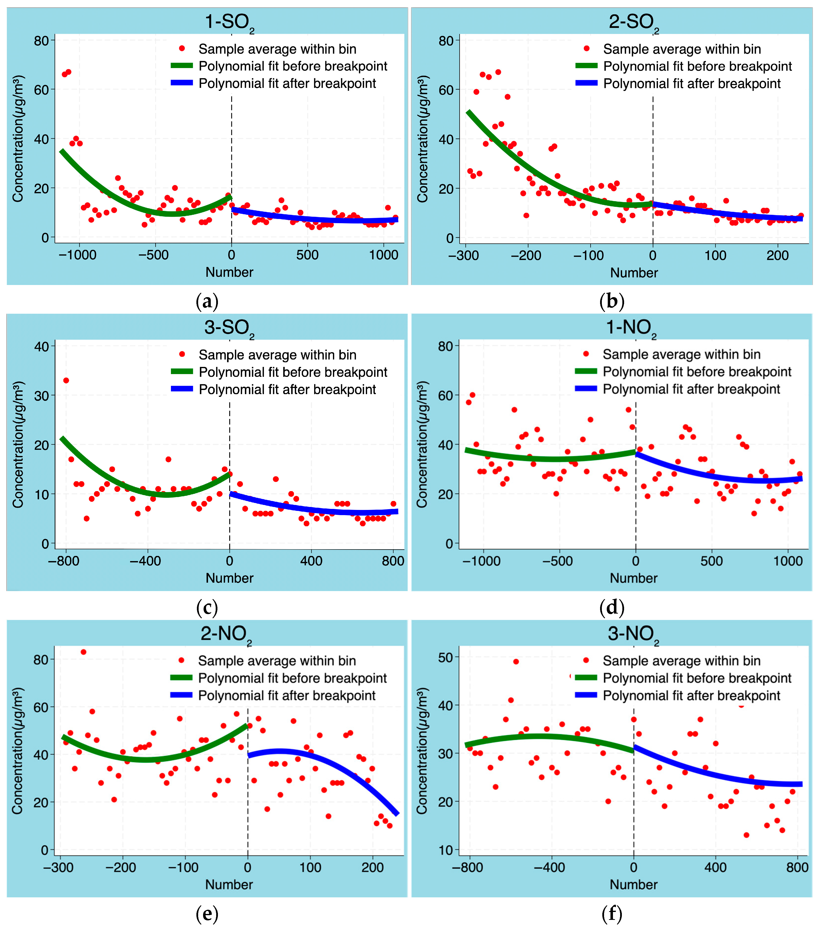
3.1. The Influence of Policy Implementation on SO₂ and NO₂

The results of computing the SO₂ concentration data using the RD model are depicted in Figure 2. The first group exhibits a relatively conspicuous demarcation point at the breakpoint, with a marked trend variation before and after the breakpoint. The green curve (prior to policy implementation) indicates a higher SO₂ concentration, while the blue curve (post-policy implementation) drops and stabilizes, suggesting a significant control effect of the policy on SO₂ concentration. The second group has no obvious demarcation point at the breakpoint, and the trend change before and after the breakpoint is relatively smooth. Although a decreasing trend in concentration can be observed, the significance of the breakpoint is not as pronounced as in other periods. The third group has a relatively distinct demarcation point at the breakpoint, with a significant trend variation before and after the breakpoint. On the whole, the policy implementation has a notable control effect on the SO₂ concentration. Although the effect is weaker in the second group, this might be attributed to seasonal factors, resulting in an insignificant reduction in concentration.

The results of calculating the NO₂ concentration data using the RD model are presented in Figure 2. The first group has no obvious demarcation point at the breakpoint, and the trend change before and after the breakpoint is relatively smooth. The NO₂ concentration was higher before policy implementation and decreased and stabilized after policy implementation, indicating a significant control effect of the policy on NO₂ concentration. The second group has a distinct demarcation point at the breakpoint, with a notable trend change before and after the breakpoint, suggesting that the policy implementation transformed the NO₂ concentration from an upward trend to a downward trend, with a significant control effect on NO₂ concentration. The third group has no obvious demarcation point at the breakpoint. Although a decreasing trend in concentration can be observed, the significance of the breakpoint is not as evident as in other periods. Overall, the policy implementation effectively improved the NO₂ concentration. Particularly in the second group, even during the winter when the concentration of polluting gases is relatively high, the control effect of the policy is more pronounced, indicating that the policy achieved relatively significant results in controlling air pollution and effectively enhanced air quality.

The fitted curves in Figure 2c,e exhibit significant jumps at the breakpoints, whereas the curves in Figure 2b,f are notably smoother. This discrepancy is primarily attributed to the timing of policy implementation in December 2017. Specifically, the observation period for SO₂ in Figure 2c spans from March to November, creating a one-year gap before and after the breakpoint. SO₂ emissions originate directly from the combustion of sulfur in fuel oil, and their concentrations can decrease markedly within a short timeframe following policies that restrict sulfur content in fuel oil or reduce ship fuel consumption. Consequently, this leads to a steep change trend in the fitted curve. In contrast, NO₂ emissions mainly result from the combustion of marine diesel oil and can react with O₃ and other oxidants in the atmosphere to establish a dynamic equilibrium. As a result, the impact of the policy on NO₂ levels is not immediate but rather manifests gradually after an adjustment period, leading to a relatively stable change trend. Interestingly, the fitted curve in Figure 2e also shows a significant jump at the breakpoint. However, the actual sampling points do not exhibit such a large jump but instead show a gentle downward trend. This phenomenon is likely due to the substantial decrease in the observed values before and after the breakpoint during the observation period, which results in a pronounced jump in the fitted curve.

The results of the RD quantification analysis of SO₂ are presented in

Table 2. Polynomial regression results of SO₂.

	1-SO2		2-SO2		3-SO2
	(a)	(b)	(a)	(b)	(a)	(b)
r	−9.60 *** (1.50)	−8.06 *** (1.46)	−6.78 ** (2.68)	−4.81 ** (2.14)	−4.51 *** (0.82)	−2.89 *** (0.82)
Cons.	24.40 *** (1.34)	24.39 *** (1.96)	20.17 *** (2.01)	23.85 *** (2.94)	16.68 *** (0.53)	19.02 *** (1.04)
IDE		−0.06 (0.05)		0.01 (0.10)		−0.18 *** (0.03)
ISE		0.07 ** (0.03)		0.01 (0.05)		0.12 *** (0.01)
IWE		−0.14 * (0.07)		−0.37 *** (0.12)		−0.20 *** (0.04)
Obs.	2187	2187	538	538	1649	1649
R2	0.718	0.732	0.774	0.780	0.663	0.671
AIC	13,023.29	12,915.82	3541.99	3529.52	8457.41	8420.76
BIC	13,068.81	12,978.41	3584.87	3580.98	8500.68	8480.25
Order	9	9	9	9	7	7

Values in parentheses are the standard deviations corrected for autocorrelation and heteroscedasticity; *, **, and *** indicate significant values at 10, 5, and 1%, respectively. The regression models (a) and (b) were fitted without and with covariates; IDE, ISE, and IWE, respectively, refer to the industrial dust emissions, industrial SO₂ emissions, and industrial wastewater emissions. Cons. represents the constant term. Obs. denotes sample size, while R² indicates goodness of fit. AIC represents the Akaike information criterion value, and BIC represents the Bayesian information criterion value. Order is the order of f(x_t).

. In the first group, r is significantly negative, suggesting that the ship lock passage policy has a marked reduction effect on the SO₂ concentration. Compared with the second and third groups, the policy effect in the first group is stronger (with a larger absolute value of r). After incorporating control variables, the absolute value of r slightly decreases, and the explanatory power of the control variables for the result is relatively minor. In the second group, r is not significant whether control variables are included or not, indicating that the influence of ship activities or the policy on the SO₂ concentration is insignificant or negligible, and the impact of control variables on the outcome variable is also small. In the third group, r is negative and significant in both models, indicating that the ship lock passage policy significantly decreased the SO₂ concentration. After adding control variables, the absolute value of r reduces but the regression values among the data groups do not vary significantly, which implies that the control variables, such as industrial smoke and dust emissions, industrial SO₂ emissions, and industrial wastewater emissions, have a relatively limited influence on the SO₂ concentration in the air at the wharf. Whether control variables are considered or not, the r value in each group of data is negative. This indicates that, in contrast to the influence of the control variables, the reduction effect of policy implementation on the SO₂ concentration is robust, and the experimental results are not prone to interference.

The results of the RD quantification analysis of NO₂ are presented in

Table 3. Polynomial regression results of NO₂.

	1-NO2		2-NO2		3-NO2
	(a)	(b)	(a)	(b)	(a)	(b)
r	−20.31 *** (3.38)	−18.52 *** (3.32)	−21.38 *** (6.22)	−21.94 *** (6.47)	−9.75 *** (3.10)	−9.37 *** (3.47)
Cons.	74.19 *** (2.10)	56.59 *** (3.92)	76.55 *** (3.29)	73.05 *** (6.10)	54.24 *** (2.34)	43.01 *** (3.74)
IDE		0.84 *** (0.15)		0.06 (0.21)		0.61 *** (0.13)
ISE		−0.06 ** (0.02)		0.048 (0.04)		−0.17 *** (0.05)
IWE		−0.75 *** (0.14)		−0.10 (0.22)		−0.16 (0.13)
Obs.	2187	2187	538	538	1649	1649
R2	0.420	0.445	0.439	0.441	0.379	0.388
AIC	15,395.96	15,300.48	3974.99	3975.72	11,080.51	11,057.79
BIC	15,441.48	15,363.07	4017.87	4031.46	11,123.78	11,117.27
Order	9	9	8	8	9	9

** and *** indicate significant values at 5% and 1%.

. In the first group, the AIC and BIC values were lower after incorporating the control variables but the change in the regression coefficient was minor, suggesting that during this long-term data period, the influence of policy implementation on the NO₂ concentration was relatively stable, and the introduction effect of the control variables was relatively weak. In the third group, the addition of control variables once again led to a reduction in the AIC and BIC values, and the regression results became more reliable after including the control variables. In the second group, whether the control variables were included or not, the regression coefficients exhibited a significant negative correlation. Among them, group (b) could reduce the influence of the estimated coefficient more effectively than group (a), indicating that the control variables could effectively improve the fitting effect of the model. Regardless of whether the control variables were considered or not, the r value of each group of data was negative, the policy had a significant effect in reducing the NO₂ concentration, and the introduction of control variables (IDE, ISE, IWE) could enhance the goodness of fit of the model, suggesting that the effect of policy implementation in reducing the NO₂ concentration was positive.

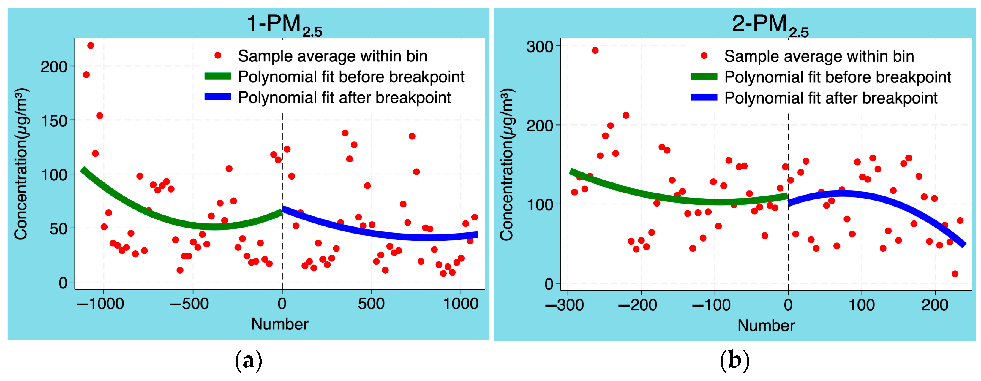
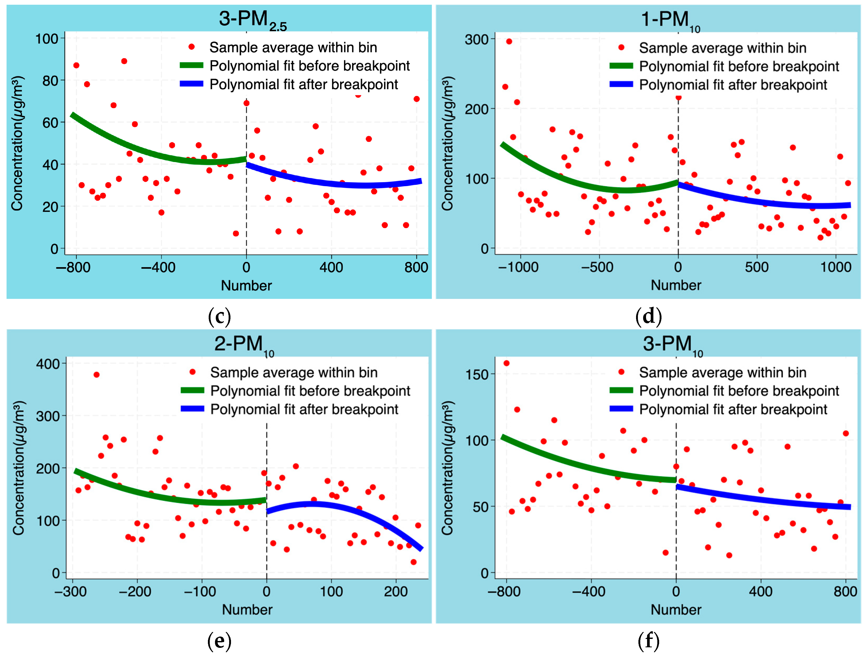
3.2. The Influence of Policy Implementation on PM_2.5 and PM₁₀

The results of computing the PM_2.5 concentration data using the RD model are depicted in Figure 3. In the first group, there is no distinct demarcation point at the breakpoint, and the trend changes before and after the breakpoint are relatively smooth. Although a downward trend in concentration can be observed, the significance of the breakpoint is not as pronounced as in other periods. In the second group, there is a relatively obvious demarcation point at the breakpoint, and the trend changes before and after the breakpoint are more pronounced. The PM_2.5 concentration was higher before the policy implementation, and it decreased significantly after the implementation, indicating that the policy implementation had a remarkable effect on controlling the PM_2.5 concentration. In the third group, there is also a relatively obvious demarcation point at the breakpoint, and the trend changes before and after the breakpoint are more distinct. Overall, the PM_2.5 concentration shows a significant downward trend after the policy implementation, and the control effect on the PM_2.5 concentration is relatively notable. The insignificant concentration decrease at the breakpoint of the data of the first group might be attributed to the higher average PM_2.5 concentration in winter.

The results of the calculation of PM₁₀ concentration data using the RD model are presented in Figure 3. In the first group, there is no pronounced demarcation point at the breakpoint, and the trend changes before and after the breakpoint are relatively smooth. Although a downward trend in concentration can be observed, the significance of the breakpoint is less conspicuous than in other periods. In the second group, there is a distinct dividing point at the breakpoint, and the trend changes before and after the breakpoint are more evident, suggesting that the policy implementation transformed the PM₁₀ concentration from an upward trend to a downward trend, exerting a significant control effect on PM₁₀ concentration. In the third group, there is a relatively obvious dividing point at the breakpoint, and the trend of concentration decline is steady. The implementation of the policy effectively ameliorated the PM₁₀ concentration. On the whole, whether it is in winter, with higher average concentrations of pollutant gases, or other seasons, the PM₁₀ concentration exhibits a stable downward trend, illustrating the effectiveness of the policy.

The results of the RD quantification analysis of PM_2.5 are presented in

Table 4. Polynomial regression results of PM_2.5.

	1-PM2.5		2-PM2.5		3-PM2.5
	(a)	(b)	(a)	(b)	(a)	(b)
r	−17.71 (14.26)	−15.10 (14.52)	−37.59 (28.15)	−24.11 (25.58)	−13.28 * (7.44)	−23.16 *** (8.59)
Cons.	174.0 *** (9.42)	213.9 *** (15.70)	155.4 *** (14.29)	189.9 *** (27.37)	90.34 *** (5.69)	106.5 *** (10.13)
IDE		−1.61 *** (0.58)		−1.08 (1.13)		−0.21 (0.37)
ISE		0.30 ** (0.15)		0.16 (0.25)		−0.24 (0.17)
IWE		0.35 (0.62)		−0.22 (1.14)		0.61 (0.42)
Obs.	2187	2187	538	538	1649	1649
R2	0.381	0.397	0.263	0.267	0.287	0.294
AIC	21,641.10	21,587.13	5581.02	5580.75	14,686.53	14,671.92
BIC	21,686.63	21,649.72	5623.89	5636.50	14,729.80	14,731.40
Order	9	9	9	9	9	9

*, **, and *** indicate significant values at 10, 5, and 1%, respectively.

. In the first group, the policy implementation has a significant influence on the concentration of PM_2.5. The regression coefficient shows a distinct negative correlation whether the control variables are incorporated or not. Particularly, in (b), after the inclusion of control variables, the regression coefficient decreases significantly, indicating that the addition of control variables significantly enhances the model-fitting effect. The influence of control variables on the PM_2.5 concentration is relatively significant during this period. Especially in the long-time series data, the inhibitory effect of policy implementation on the PM_2.5 concentration is further validated. In the second group, the AIC and BIC values also decline with the introduction of control variables, suggesting an improvement in the model fit. The regression coefficient of ISE turns negative after the inclusion of control variables and is closer to the significant level, indicating that ISE may have a certain influence on the PM_2.5 concentration. Therefore, the introduction of control variables in this group, although it does not cause a substantial change in the coefficient, significantly improves the model fit and explanatory power, reflecting the potential role of control variables on air quality. In the third group, when the control variables (IDE, ISE, IWE) are included in the model, the AIC and BIC values decrease, indicating an improvement in the model-fitting effect. However, the change in the regression coefficients is relatively small, suggesting that these control variables have a weak influence on this group of data. Numerically, the control variables have no significant impact on the regression coefficients, suggesting that in this case, the policy has a relatively stable influence on the change in the PM_2.5 concentration, and the influence of the control variables is limited. Overall, the control variables (IDE, ISE, IWE) exhibit different degrees of influence in different groups and have a potential role in air quality but are insufficient to affect the experimental conclusion. The addition of control variables significantly improves the model fit and effectively inhibits the PM_2.5 concentration.

The results of the RD quantification analysis of PM₁₀ are presented in

Table 5. Polynomial regression results of PM₁₀.

	1-PM10		2-PM10		3-PM10
	(a)	(b)	(a)	(b)	(a)	(b)
r	−49.13 *** (15.09)	−46.81 *** (15.15)	−39.03 (26.82)	−21.40 (24.28)	−55.31 *** (11.44)	−57.63 *** (11.95)
Cons.	211.5 *** (9.63)	246.5 *** (16.11)	192.8 *** (14.41)	233.6 *** (31.30)	127.9 *** (7.32)	159.2 *** (14.54)
IDE		−0.99 * (0.58)		−1.55 (1.29)		−0.33 (0.52)
ISE		0.31 * (0.17)		0.28 (0.28)		−0.09 (0.24)
IWE		−0.92 (0.66)		−0.01 (1.33)		−0.55 (0.56)
Obs.	2187	2187	538	538	1649	1649
R2	0.390	0.403	0.353	0.356	0.283	0.299
AIC	22,372.91	22,329.05	5760.36	5758.96	15,896.35	15,863.89
BIC	22,424.12	22,397.34	5807.52	5814.70	15,945.02	15,928.79
Order	9	1	9	9	8	9

* and *** indicate significant values at 10% and 1%.

. In the first group, the introduction of control variables significantly enhanced the model fit, with the AIC and BIC values decreasing. IDE exhibited a significant negative correlation with the PM₁₀ concentration, while the influence of ISE and IWE on the concentration was relatively minor. Overall, the control variables more conspicuously improved the model fit in this group, demonstrating the efficacy of the policy. In the second group, the inclusion of control variables also ameliorated the model fit. IDE had a distinct positive impact on the PM₁₀ concentration while the effects of ISE and IWE were relatively small, but the positive regression coefficient of ISE indicated its latent effect. The role of control variables in this group was more intricate but it still enhanced the fitting effect. In the third group, after the addition of control variables (IDE, ISE, IWE), the AIC and BIC values decreased significantly, suggesting an improvement in the model-fitting effect. Among the regression coefficients, IDE had a significant positive influence on the PM₁₀ concentration, while IWE manifested a certain negative influence. Overall, the incorporation of control variables significantly enhanced the model fit and verified the effective inhibitory effect of policy implementation on the PM₁₀ concentration.

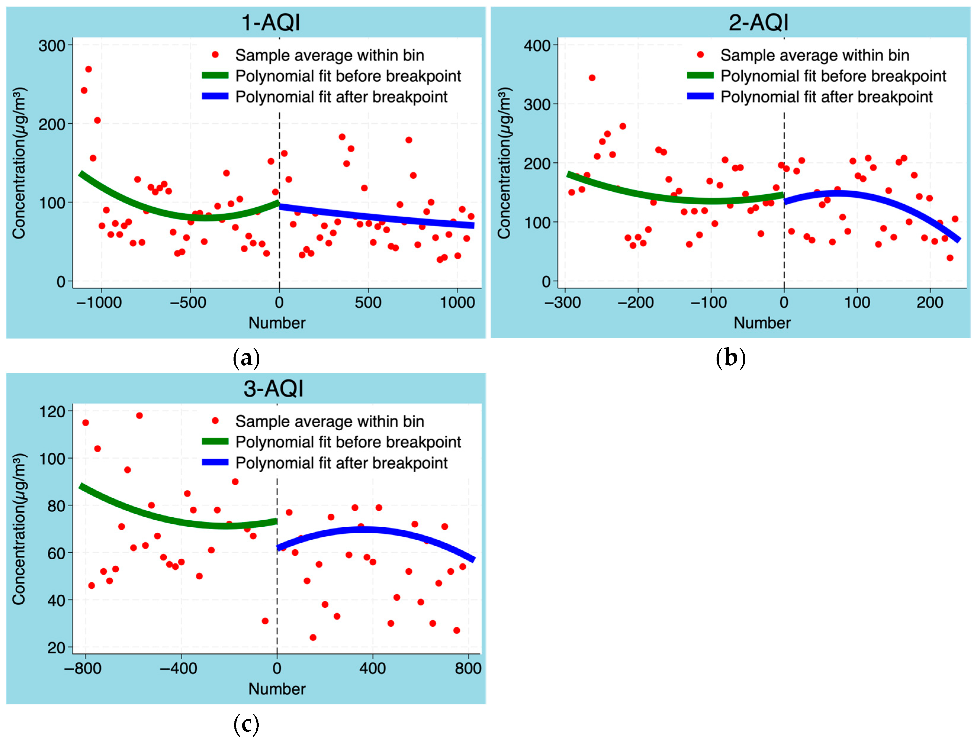
3.3. The Influence of Policy Implementation on AQI

The results of computing the AQI concentration data using the RD model are depicted in Figure 4. The first group presents no distinct demarcation point at the breakpoint but maintains a stable downward trend after the breakpoint. The second group has a relatively obvious demarcation point at the breakpoint, and the trend changes significantly before and after the breakpoint. The AQI concentration was relatively high before the policy implementation, and a marked downward trend was exhibited after the policy implementation, indicating that the policy implementation has a significant control effect on the AQI concentration. The third group also has a distinct demarcation point at the breakpoint, and the trend changes significantly before and after the breakpoint. On the whole, regardless of whether it is in winter, with higher average concentrations of pollutant gases, or other seasons, all three groups of data maintain a stable downward trend after the breakpoint, suggesting that the policy implementation effectively enhanced the air quality in Yichang City and has a notable effect on improving the AQI value.

The results of the quantile regression analysis of the AQI are presented in

Table 6. Polynomial regression results of the Air Quality Index (AQI).

	1-AQI		2-AQI		3-AQI
	(a)	(b)	(a)	(b)	(a)	(b)
r	−20.12 (16.36)	−17.92 (16.45)	−40.17 (34.07)	−25.14 (31.22)	−43.35 *** (9.60)	−44.62 *** (9.86)
Cons.	208.7 *** (10.46)	251.6 *** (17.49)	198.6 *** (18.60)	244.0 *** (34.75)	110.3 *** (6.52)	141.3 *** (12.11)
IDE		−1.61 ** (0.64)		−1.35 (1.42)		−0.71 * (0.43)
ISE		0.35 ** (0.16)		0.15 (0.29)		0.21 (0.21)
IWE		−0.10 (0.70)		−0.22 (1.41)		−0.78 (0.49)
Obs.	2187	2187	538	538	1649	1649
R2	0.325	0.340	0.254	0.259	0.157	0.168
AIC	22,324.73	22,279.16	5787.93	5785.12	15,439.75	15,420.65
BIC	22,375.94	22,347.45	5835.10	5840.86	15,488.42	15,485.54
Order	9	9	9	9	8	8

*, **, and *** indicate significant values at 10, 5, and 1%, respectively.

. In the first group, regardless of the inclusion of control variables, the regression coefficients exhibit a negative correlation trend, and the introduction of control variables significantly reduces the AIC and BIC values. The regression coefficient of IDE is negative and approaches the significant level while the influence of ISE and IWE is relatively small, but ISE shows a slight positive relationship. The incorporation of control variables significantly enhances the model’s fitting effect, particularly in the variation of AQL values, where the negative impact of IDE is more pronounced. In the second group, the addition of control variables also lowers the AIC and BIC values, indicating an improvement in the model’s fitting effect. Among the regression coefficients, the influence of IDE on AQL remains negative but its significance decreases. The regression coefficients of ISE and IWE are relatively small; especially, ISE shows a slight positive relationship, suggesting that ISE may have a positive contribution to air quality. On the whole, the inclusion of control variables in this group improved the model but the effect is relatively weak. In the third group, after including the control variables (IDE, ISE, IWE), both the AIC and BIC values decrease, indicating an enhancement in the model’s fitting effect. The regression coefficients show that the influence of IDE on AQL is negative and significant. While the regression coefficients of ISE and IWE are relatively small, their influence is rather limited. Overall, the inclusion of control variables significantly improves the model fitting. The negative influence of IDE on AQL is relatively prominent, demonstrating the positive impact of policy implementation on AQI and the positive effect of policy implementation on the improvement of air quality.

4. Robustness Tests

The purpose of conducting robustness tests is to ensure the adaptability of the regression model to different datasets, model settings, and methods, thereby enhancing the reliability and accuracy of the results. Different robustness testing methods help verify the robustness of the model from various perspectives and reduce potential biases and errors when the model is confronted with different situations. This study employed local linear regression based on rectangular kernel functions, local linear regression based on triangular kernel functions, polynomial order tests, and continuity tests of control variables.

4.1. Polynomial Order Test

When the polynomial function f(x_t) assumes different continuous orders, if the estimation results of the RD model remain stable and invariant, it suggests that the variation in the polynomial order has no significant influence on the robustness of the RD results. In the relevant studies of SO₂, NO₂, and particulate matter, only the regression results corresponding to the polynomial order with the minimum AIC or BIC value were presented, without displaying the fitting results of all orders. This study further validates the robustness of the regression model by selecting the second and third-order fitting results of AIC or BIC and combining IDE, ISE, and IWE as the control variables. The regression results are shown in

Table 7. Polynomial regression test results of SO₂.

	1-SO2		2-SO2		3-SO2
	(a)	(b)	(a)	(b)	(a)	(b)
r	−8.93 *** (1.33)	−1.25 (1.07)	−2.35 (2.07)	−1.72 (2.01)	−2.31 ** (0.94)	−3.43 *** (1.05)
Cons.	20.91 *** (2.09)	26.54 *** (1.85)	23.99 *** (2.81)	23.95 *** (2.76)	20.09 *** (0.98)	20.28 *** (1.13)
IDE	0.03 (0.07)	−0.35 *** (0.06)	−0.08 (0.09)	−0.09 (0.09)	−0.20 *** (0.03)	−0.20 *** (0.03)
ISE	0.09 *** (0.03)	0.15 *** (0.03)	0.04 (0.04)	0.04 (0.04)	0.10 *** (0.01)	0.13 *** (0.01)
IWE	−0.38 *** (0.05)	−0.13 (0.08)	−0.46 *** (0.10)	−0.44 *** (0.11)	−0.06 (0.04)	−0.16 *** (0.04)
Obs.	2187	2187	538	538	1649	1649
Order	8	7	7	8	9	8

** and *** indicate significant values at 5% and 1%. (a) and (b) represent different orders of the polynomial order test.

,

Table 8. Polynomial regression test results of NO₂.

	1-NO2		2-NO2		3-NO2
	(a)	(b)	(a)	(b)	(a)	(b)
r	−20.26 *** (3.28)	−9.03 *** (3.14)	−18.79 *** (6.14)	−23.42 *** (6.86)	−16.99 *** (3.53)	−10.69 *** (3.33)
Cons.	52.74 *** (3.73)	61.50 *** (3.54)	74.65 *** (6.07)	74.26 *** (6.06)	44.54 *** (4.18)	43.11 *** (4.05)
IDE	0.98 *** (0.15)	0.37 *** (0.12)	−0.05 (0.22)	0.03 (0.21)	0.61 *** (0.14)	0.57 *** (0.14)
ISE	−0.04 (0.03)	0.05 ** (0.02)	0.07 (0.04)	0.04 (0.04)	−0.02 (0.06)	−0.11 ** (0.05)
IWE	−1.03 *** (0.12)	−0.71 *** (0.11)	−0.11 (0.22)	−0.01 (0.20)	−0.77 *** (0.13)	−0.46 *** (0.14)
Obs.	2187	2187	538	538	1649	1649
Order	8	6	9	7	8	7

** and *** indicate significant values at 5% and 1%.

,

Table 9. Polynomial regression test results of PM_2.5.

	1-PM2.5		2-PM2.5		3-PM2.5
	(a)	(b)	(a)	(b)	(a)	(b)
r	22.69 * (12.67)	−22.64 * (13.27)	−8.54 (27.07)	−0.16 (25.45)	−28.70 *** (8.50)	−30.73 *** (9.04)
Cons.	186.9 *** (15.17)	219.7 *** (14.35)	195.3 *** (26.34)	191.4 *** (26.77)	104.0 *** (10.94)	106.2 *** (11.17)
IDE	−3.10 *** (0.52)	−0.73 (0.60)	−1.98 * (1.07)	−2.01 * (1.08)	−0.15 (0.40)	−0.19 (0.40)
ISE	0.86 *** (0.13)	0.46 *** (0.14)	0.39 * (0.22)	0.40 * (0.22)	−0.09 (0.18)	−0.05 (0.20)
IWE	−0.39 (0.54)	−1.51 *** (0.54)	−0.58 (1.06)	−0.66 (1.12)	−0.19 (0.45)	−0.23 (0.44)
Obs.	2187	2187	538	538	1649	1649
Order	8	6	7	8	7	8

* and *** indicate significant values at 10% and 1%.

,

Table 10. Polynomial regression test results of PM₁₀.

	1-PM10		2-PM10		3-PM10
	(a)	(b)	(a)	(b)	(a)	(b)
r	−54.86 *** (14.64)	1.52 (13.17)	16.06 (23.26)	6.98 (24.96)	−46.17 *** (11.38)	−31.81 *** (11.79)
Cons.	222.0 *** (15.68)	258.9 *** (14.92)	231.0 *** (27.77)	236.0 *** (31.56)	149.6 *** (13.05)	155.6 *** (13.94)
IDE	−0.17 (0.59)	−3.03 *** (0.53)	−2.68 ** (1.11)	−2.61 ** (1.24)	−0.37 (0.51)	−0.23 (0.49)
ISE	0.47 *** (0.16)	0.97 *** (0.15)	0.53 ** (0.21)	0.57 ** (0.26)	−0.27 (0.23)	−0.57 ** (0.22)
IWE	−2.65 *** (0.57)	−1.49 ** (0.58)	−0.31 (1.15)	−0.55 (1.30)	−0.02 (0.57)	1.20 ** (0.55)
Obs.	2187	2187	538	538	1649	1649
Order	8	6	6	8	9	7

** and *** indicate significant values at 5% and 1%.

and

Table 11. Polynomial regression test results of AQI.

	1-AQI		2-AQI		3-AQI
	(a)	(b)	(a)	(b)	(a)	(b)
r	−25.70 (15.67)	20.31 (14.83)	−7.08 (32.60)	1.15 (30.79)	−41.54 *** (9.72)	−38.21 *** (9.35)
Cons.	220.4 *** (16.97)	266.3 *** (17.11)	249.2 *** (33.50)	245.0 *** (33.99)	145.0 *** (12.26)	141.3 *** (12.11)
IDE	−0.61 (0.66)	−3.24 *** (0.59)	−2.33 * (1.33)	−2.35 * (1.35)	−0.86 ** (0.43)	−0.74 * (0.43)
ISE	0.54 *** (0.16)	0.83 *** (0.16)	0.40 (0.25)	0.41 (0.25)	0.16 (0.20)	0.12 (0.20)
IWE	−2.24 *** (0.61)	−0.15 (0.73)	−0.62 (1.31)	−0.71 (1.38)	−0.37 (0.45)	−0.50 (0.50)
Obs.	2187	2187	538	538	1649	1649
Order	8	7	7	8	6	7

*, **, and *** indicate significant values at 10%, 5%, and 1%.

.

4.2. Local Linear Regression Test Based on Rectangular Kernel Function

The regression results are shown in

Table 12. Local linear regression results based on rectangular kernel function.

	1-SO2	2-SO2	3-SO2	1-NO2	2-NO2	3-NO2
r-Treat	2.45	1.75	−2.22	−10.18	−12.98	−16.13
r-0.5Treat	4.26	4.26	−0.4	4.2	−4.22	4
r-2Treat	0.02	0.76	−4.25	−17.12	−19.38	−17.75
Obs.	2187	538	1649	2187	538	1649
Bandwidth	6.95	7.07	6.01	8.69	10.18	7.70
0.5Bandwidth	3.47	3.53	3.00	4.34	5.09	3.85
2Bandwidth	13.90	14.14	12.03	17.39	20.37	15.40
	1-PM2.5	2-PM2.5	3-PM2.5	1-PM10	2-PM10	3-PM10
r-Treat	50.16	53.88	−36.75	43.11	37.18	−71.80
r-0.5Treat	59.61	35.10	−23.25	9.06	32.56	−39.04
r-2Treat	24.05	13.28	−16.87	7.01	7.16	−33.34
Obs.	2187	538	1649	2187	538	1649
Bandwidth	11.12	13.76	10.34	12.84	16.05	11.59
0.5Bandwidth	5.56	6.88	5.17	6.42	8.02	5.79
2Bandwidth	22.24	27.52	20.69	25.69	32.10	23.18
	1-AQI	2-AQI	3-AQI
r-Treat	65.91	73.74	−41.42
r-0.5Treat	74.72	45.79	−26.98
r-2Treat	31.85	11.13	−41.42
Obs.	2187	538	1649
Bandwidth	11.87	15.13	10.82
0.5Bandwidth	5.93	7.56	5.41
2Bandwidth	23.75	30.27	21.64

Bandwidth, 0.5Bandwidth, and 2Bandwidth represent the optimal bandwidth, half of the optimal bandwidth, and twice the optimal bandwidth, respectively. Treat, 0.5Treat, and 2Treat, respectively, represent the results of breakpoint regression analysis conducted with half and twice the optimal bandwidth.

. In the first group, the regression coefficients of the concentrations of SO₂, NO₂, PM_2.5, and PM₁₀ and the AQI value did not exhibit a negative correlation. The implementation of the policy should have reduced the emissions of pollutant gases; however, the regression results did not reveal a distinct downward trend. This might be attributed to the selected breakpoint being in winter when the average concentration of pollutants was relatively high or the pollution sources underwent changes in the initial stage of policy implementation. In the second group, the regression coefficients of the concentrations of SO₂, NO₂, PM_2.5, and PM₁₀ and the AQI value did not demonstrate a strong negative correlation, suggesting that the concentrations of various gases and the AQI value did not significantly decrease after the policy was executed. In the third group, the regression coefficients displayed substantial negative values. As time elapsed, the policy effect began to manifest, and the overall air quality improved. This indicates that the implementation of the policy effectively decreased the concentrations of SO₂, NO₂, PM_2.5, and PM₁₀ and the AQI value, and the sensitivity of each concentration value to the change in bandwidth was relatively low. The selection of different bandwidths had a minor impact on the regression model, indicating that the regression results were robust. The policy demonstrated a significant effect in reducing the concentrations of SO₂, NO₂, PM_2.5, and PM₁₀ and the AQI value. The results indicate that the regression model exhibited strong robustness in the prediction of multiple pollutants and time periods and concurrently verified the effective control effect of the policy on pollutant concentrations.

4.3. Local Linear Regression Test Based on Triangular Kernel Function

The policy effects of different pollutants during different time periods and under various bandwidths are largely consistent with the analysis results of the rectangular kernel function, yet exhibit a smoother changing trend. The regression results are shown in

Table 13. Local linear regression results based on triangular kernel function.

	1-SO2	2-SO2	3-SO2	1-NO2	2-NO2	3-NO2
r-Treat	2.60	2.55	−1.91	−9.83	−11.89	−15.23
r-0.5Treat	4.95	4.96	−0.42	−0.08	−2.89	−2.81
r-2Treat	1.10	1.07	−4.11	−16.09	−16.24	−17.50
Obs.	2187	538	1649	2187	538	1649
Bandwidth	8.84	9.00	7.66	11.07	12.96	9.80
0.5Bandwidth	4.42	4.50	3.83	5.53	6.48	4.90
2Bandwidth	17.69	18.01	15.32	22.14	25.93	19.61
	1-PM2.5	2-PM2.5	3-PM2.5	1-PM10	2-PM10	3-PM10
r-Treat	48.20	48.01	−32.75	38.41	30.46	−62.95
r-0.5Treat	44.31	40.02	−19.29	20.08	27.46	−34.62
r-2Treat	26.76	18.93	−16.30	15.24	10.03	−40.28
Obs.	2187	538	1649	2187	538	1649
Bandwidth	14.16	17.51	13.17	16.35	20.43	14.76
0.5Bandwidth	7.08	8.75	6.58	8.17	10.21	7.38
2Bandwidth	28.32	35.03	26.35	32.70	40.87	29.52
	1-AQI	2-AQI	3-AQI
r-Treat	64.47	60.99	−36.70
r-0.5Treat	52.78	52.42	−19.87
r-2Treat	32.92	19.09	−15.97
Obs.	2187	538	1649
Bandwidth	15.12	19.27	13.77
0.5Bandwidth	7.56	9.63	6.88
2Bandwidth	30.24	38.54	27.55

Bandwidth, 0.5Bandwidth, and 2Bandwidth represent the optimal bandwidth, half of the optimal bandwidth, and twice the optimal bandwidth, respectively. Treat, 0.5Treat, and 2Treat, respectively, represent the results of breakpoint regression analysis conducted with half and twice the optimal bandwidth.

. In the first group, the regression coefficients of the concentrations of SO₂, NO₂, PM_2.5, and PM₁₀ and the AQI value do not display a strong negative correlation. The implementation of the policy has no significant reduction effect on the concentrations of these pollutants and the AQI value. Nevertheless, the regression results herein do not show a distinct downward trend, which might be attributed to the influence of other pollution sources at the port, such as industrial emissions or local ship activities, or the relatively short implementation period of the policy, which has not yet fully manifested a significant impact. In the second group, the regression coefficients indicate that the concentrations of various pollutants did not significantly decrease after the policy was implemented. The consistency of the regression coefficients after adjusting the bandwidth is relatively high, suggesting that the bandwidth has a relatively minor impact on the regression model, further verifying the stability of the model. In the third group, the regression results of the concentrations of SO₂, NO₂, PM_2.5, and PM₁₀ and the AQI value reveal a strong negative correlation in the regression coefficients, suggesting that in the long term, the concentrations of various gases and the AQI value significantly decreased after the policy was implemented. The consistency of the regression coefficients after adjusting the bandwidth is relatively high. The regression model demonstrates strong robustness and adaptability in the prediction of multiple pollutants and time periods, enhancing the reliability and accuracy of the results. This indicates that the policy can stably reflect the effective control effect of the policy on pollutant concentrations. Meanwhile, the significant negative values of the regression coefficients also confirm the effectiveness of the policy, effectively improving the air quality in Yichang City.

4.4. Continuity Test for Covariates

In order to ensure that the control variables in the regression model are not biased due to other potential factors or external disturbances, a continuity test of the control variables was employed in this study. Based on the polynomial regression results, including the control variables in Section 3, it can be speculated that the collected data of the SO₂, NO₂, PM_2.5, and PM₁₀ concentrations and the AQI values might be influenced by IDE, ISE, and IWE during the monitoring period. Hence, the control variables IDE, ISE, and IWE were selected for polynomial regression tests.

The regression results are shown in

Table 14. Continuity test of covariates.

	1			2			3
	IDE	ISE	IWE	IDE	ISE	IWE	IDE	ISE	IWE
r	−5.46 *** (0.72)	−26.57 *** (3.12)	−2.69 *** (0.36)	3.86 *** (1.24)	−1.09 (4.42)	2.07 * (1.06)	−3.95 *** (0.73)	−8.41 *** (2.67)	−4.09 *** (0.64)
Cons.	42.43 *** (0.60)	77.47 *** (2.85)	15.95 *** (0.24)	37.64 *** (0.97)	61.91 *** (3.64)	12.76 *** (0.96)	41.45 *** (0.39)	65.47 *** (1.21)	15.88 *** (0.24)
Obs.	2187	2187	2187	538	538	538	1649	1649	1649
R2	0.937	0.908	0.919	0.940	0.895	0.933	0.946	0.953	0.919
Order	8	9	7	9	9	9	8	8	7

* and *** indicate significant values at 10% and 1%.

. In the first group, IDE, ISE, and IWE exhibit a significant negative correlation, featuring a favorable fitting effect and a relatively prominent influence. In the second group, IDE reveals a minor positive correlation, suggesting that its impact on the dependent variable during this period is relatively mild. ISE presents a negative correlation, yet its coefficient is small, indicating a relatively insignificant influence. IWE, although demonstrating a negative correlation, has a smaller influence compared to other variables. In the third group, IDE, ISE, and IWE possess a significant negative correlation, exerting a relatively notable influence on the dependent variable, and the model-fitting effect is stable. Owing to the stability of the analysis results, the conclusions drawn possess a high level of credibility. Particularly, after considering the control variables, the control effect of the policy implementation on the concentration of polluting gases has been further verified. Even under different model settings, the positive influence of the policy on air quality remains significant, substantiating the effectiveness of the policy in enhancing the air quality of Yichang City.

5. Conclusions

This study verified the significant improvement effect of the Linked Control Policy for Vessels Passing Through Locks on air quality using the RD model. The analysis based on the air quality monitoring data of Yichang City from 2014 to 2020 indicates that the concentrations of major pollutants showed a systematic decline after the policy’s implementation. Specifically, the concentration of SO₂ dropped by 67%, NO₂ dropped by 32%, PM_2.5 dropped by 42%, and PM₁₀ dropped by 46%, while the comprehensive Air Quality Index (AQI) improved by 27%. This study established the causal relationship between policy intervention and the reduction of pollutant concentrations through robustness tests, confirming that by optimizing the lock ship process and reducing the idle time of diesel engines at the lock, the direct impact of shipping emissions on the atmospheric environment of cities along the river can be effectively curbed. This discovery provides direct empirical evidence for the green management of inland shipping.

This study is the first to systematically disclose the environmental benefits of the “soft” management policy of optimizing the lock passage process. The existing literature mostly pays attention to the emission reduction effects of upgrading technical equipment, while this study discovers that significant environmental benefits can be achieved merely through innovative scheduling strategies. Particularly worthy of attention is that the prominent reduction of SO₂ (67%) far exceeds that of other pollutants. This might be attributed to the synergy with the policy controlling the sulfur content of fuel used by vessels waiting for lock passage, suggesting the superimposed and enhanced effect of combined policy tools [35].

However, this study does have certain limitations. For example, the monitoring data did not differentiate the contributions of shipping sources from those of other pollution sources, potentially underestimating the actual effect of the policy. Therefore, if there are emission sources such as volcanoes or large-scale power plants in other areas, the research method proposed in this paper requires the collection of more sufficient data and more refined modeling. Meanwhile, the research period encompassed the early stage of the COVID-19 pandemic, and the special socio–economic activities during this time might have exerted confounding effects [36,37]. Furthermore, the applicability of the conclusions to the ship locks in the plain river sections requires further verification. Subsequent studies could combine the AIS trajectories of ships with emission inventories to construct source apportionment models and expand to multiple hubs in the middle reaches of the Yangtze River for comparative research. At the same time, it is recommended that health benefit assessment and economic cost analysis be included in the policy evaluation system to provide multi-dimensional decision support for the optimization of green shipping policies. In order to further enhance the effectiveness of the joint control policy for ships passing through the lock, the use of generative artificial intelligence models can be considered to propose more efficient lock passage strategies. This direction is worthy of in-depth study.

References

1. Zhang, Y.; Yang, X.; Brown, R.; Yang, L.; Morawska, L.; Ristovski, Z.; Fu, Q.; Huang, C. Shipping emissions and their impacts on air quality in China. Sci. Total Environ. 2017, 581, 186–198. [Google Scholar] [PubMed]
2. Liu, Y.S.; Ge, Y.S.; Tan, J.W.; Fu, M.L.; Shah, A.N.; Li, L.Q.; Ji, Z.; Ding, Y. Emission characteristics of offshore fishing ships in the Yellow Bo Sea, China. J. Environ. Sci. 2018, 65, 83–91. [Google Scholar]
3. Mueller, N.; Westerby, M.; Nieuwenhuijsen, M. Health Impact Assessments of Shipping and Port-Sourced Air Pollution on a Global Scale: A Scoping Literature Review. Environ. Res. 2023, 216, 114460. [Google Scholar] [PubMed]
4. Matthias, V.; Bewersdorff, I.; Aulinger, A.; Quante, M. The contribution of ship emissions to air pollution in the North Sea regions. Environ. Pollut. 2010, 158, 2241–2250. [Google Scholar]
5. Zhang, X.; Aikawa, M. The Variation of PM2.5 from Ship Emission under Low-Sulfur Regulation: A Case Study in the Coastal Suburbs of Kitakyushu, Japan. Sci. Total Environ. 2023, 858, 159968. [Google Scholar]
6. Sofiev, M.; Winebrake, J.J.; Johansson, L.; Carr, E.W.; Prank, M.; Soares, J.; Vira, J.; Kouznetsov, R.; Jalkanen, J.-P.; Corbett, J.J. Cleaner Fuels for Ships Provide Public Health Benefits with Climate Tradeoffs. Nat. Commun. 2018, 9, 406. [Google Scholar]
7. Yuan, T.; Song, H.; Wood, R.; Wang, C.; Oreopoulos, L.; Platnick, S.E.; Von Hippel, S.; Meyer, K.; Light, S.; Wilcox, E. Global Reduction in Ship-Tracks from Sulfur Regulations for Shipping Fuel. Sci. Adv. 2022, 8, eabn7988. [Google Scholar]
8. Liu, H.; Fu, M.; Jin, X.; Shang, Y.; Shindell, D.; Faluvegi, G.; Shindell, C.; He, K. Health and Climate Impacts of Ocean-Going Vessels in East Asia. Nat. Clim. Chang. 2016, 6, 1037–1041. [Google Scholar]
9. Zhou, F.; Hou, L.; Zhong, R.; Chen, W.; Ni, X.; Pan, S.; Zhao, M.; An, B. Monitoring the Compliance of Sailing Ships with Fuel Sulfur Content Regulations Using Unmanned Aerial Vehicle (UAV) Measurements of Ship Emissions in Open Water. Atmos. Meas. Tech. 2020, 13, 4899–4909. [Google Scholar]
10. Fu, M.; Ding, Y.; Ge, Y.; Yu, L.; Yin, H.; Ye, W.; Liang, B. Real-World Emissions of Inland Ships on the Grand Canal, China. Atmos. Environ. 2013, 81, 222–229. [Google Scholar] [CrossRef]
11. Kurtenbach, R.; Vaupel, K.; Kleffmann, J.; Klenk, U.; Schmidt, E.; Wiesen, P. Emissions of NO, NO2, and PM from Inland Shipping. Atmos. Chem. Phys. 2016, 16, 14285–14295. [Google Scholar]
12. Zhou, F.; Wang, Y.; Hou, L.; An, B. Air Pollutant Emission Factors of Inland River Ships under Compliance. J. Mar. Sci. Eng. 2024, 12, 1732. [Google Scholar] [CrossRef]
13. Wang, X.; Zhao, Y.; Sun, P.; Wang, X. An Analysis on Convergence of Data-Driven Approach to Ship Lock Scheduling. Math. Comput. Simul. 2013, 88, 31–38. [Google Scholar]
14. Zhao, X.; Lin, Q.; Yu, H. A Co-Scheduling Problem of Ship Lift and Ship Lock at the Three Gorges Dam. IEEE Access 2020, 8, 132893–132910. [Google Scholar]
15. Wu, Z.; Ji, B.; Yu, S.S. Modeling and Solution Algorithm for Green Lock Scheduling Problem on Inland Waterways. Mathematics 2024, 12, 1192. [Google Scholar] [CrossRef]
16. Liu, S.; Zhang, Y.; Guo, W.; Tian, H.; Tang, K. Ship Scheduling Problem Based on Channel-Lock Coordination in Flood Season. Expert Syst. Appl. 2024, 254, 124393. [Google Scholar]
17. Zhang, H.; Ke, J. An Intelligent Scheduling System and Hybrid Optimization Algorithm for Ship Locks of the Three Gorges Hub on the Yangtze River. Mech. Syst. Signal Process. 2024, 208, 110974. [Google Scholar]
18. Zhang, Y.; Zheng, Q.-Q.; He, L.-J.; Tian, H.-W. Ship Traffic Optimization Method for Solving the Approach Channel and Lock Co-Scheduling Problem of the Three Gorges Dam on the Yangzi River. Ocean Eng. 2023, 276, 114196. [Google Scholar] [CrossRef]
19. Ji, B.; Yuan, X.; Yuan, Y.; Lei, X.; Fernando, T.; Iu, H.H.C. Exact and Heuristic Methods for Optimizing Lock-Quay System in Inland Waterway. Eur. J. Oper. Res. 2019, 277, 740–755. [Google Scholar]
20. Xin, Q.; Wang, Y.; Zhang, M.; Wang, R.; Wang, Y. Quantitative Analysis of Influencing Factors on Changzhou Ship Lock Capacity. Appl. Sci. 2024, 14, 4958. [Google Scholar] [CrossRef]
21. Li, X.; Mou, J.; Chen, L.; Huang, Y.; Chen, P. Ship–Infrastructure Cooperation: Survey on Infrastructure Scheduling for Waterborne Transportation Systems. J. Mar. Sci. Eng. 2022, 11, 31. [Google Scholar] [CrossRef]
22. Schwarzkopf, D.A.; Petrik, R.; Matthias, V.; Quante, M.; Yu, G.; Zhang, Y. Comparison of the Impact of Ship Emissions in Northern Europe and Eastern China. Atmosphere 2022, 13, 894. [Google Scholar] [CrossRef]
23. Golak, J.A.P.; Defryn, C.; Grigoriev, A. Optimizing Fuel Consumption on Inland Waterway Networks: Local Search Heuristic for Lock Scheduling. Omega 2022, 109, 0305–0483. [Google Scholar]
24. Smith, L.D.; Ii, D.C.S.; Campbell, J.F. Simulation of Alternative Approaches to Relieving Congestion at Locks in a River Transportion System. Oper. Res. 2010, 50, 105–106. [Google Scholar]
25. Segovia, P.; Negenborn, R.R.; Reppa, V. Vessel Passage Scheduling through Cascaded Bridges Using Mixed-integer Programming. IFAC Pap. 2022, 55, 248–253. [Google Scholar]
26. Pang, Q.H.; Wu, X.Y. Optimization Scheduling Model of Double Line Shiplock Based on Nonlinear Goal Programming. J. Appl. Res. Technol. 2014, 12, 192–200. [Google Scholar]
27. National Economic and Social Development Statistical Bulletin of Yichang City. 2023. Available online: http://www.yichang.gov.cn/zfxxgk/show.html?aid=1&id=233339 (accessed on 8 March 2024).
28. Three Gorges Navigation Authority. The Throughput of the Three Gorges Hub Will Be Nearly 160 Million Tons in 2024. 2025. Available online: https://sxth.mot.gov.cn/xw_1/thyw_5769/202501/t20250102_427449.html (accessed on 6 January 2025).
29. Ma, Y.; Chen, D.; Fu, X.; Shang, F.; Guo, X.; Lang, J.; Zhou, Y. Impact of Sea Breeze on the Transport of Ship Emissions: A Comprehensive Study in the Bohai Rim Region, China. Atmosphere 2022, 13, 1094. [Google Scholar] [CrossRef]
30. Zhou, F.; Fan, Y.; Zou, J.; An, B. Ship Emission Monitoring Sensor Web for Research and Application. Ocean Eng. 2022, 249, 110980. [Google Scholar]
31. Three Gorges Navigation Authority. The Traffic Organization of Yangtze River Trunk Line Crossing Dam by Coordinated Control of Ships. 2017. Available online: https://sxth.mot.gov.cn/fw/thfw/thgg_5774/202103/P020210327592677984068.pdf (accessed on 6 January 2025).
32. GB 3095—2012; Ministry of Ecology and Environment Ambient Air Quality Standards. 2012. Available online: https://www.mee.gov.cn/ywgz/fgbz/bz/bzwb/dqhjbh/dqhjzlbz/201203/W020120410330232398521.pdf (accessed on 8 February 2025).
33. Zhang, Q.; Zheng, Z.; Wan, Z.; Zheng, S. Does Emission Control Area Policy Reduce Sulfur Dioxides Concentration in Shanghai? Transp. Res. Part Transp. Environ. 2020, 81, 102289. [Google Scholar]
34. Zhang, Q.; Liu, H.; Wan, Z. Evaluation on the effectiveness of ship emission control area policy: Heterogeneity detection with the regression discontinuity method. Environ. Impact Assess. Rev. 2022, 94, 106747. [Google Scholar]
35. Song, S.K.; Shon, Z.H.; Moon, S.H.; Lee, T.H.; Kim, H.S.; Kang, S.H.; Park, G.H.; Yoo, E.C. Impact of international Maritime Organization 2020 sulfur content regulations on port air quality at international hub port. J. Clean. Prod. 2022, 347, 131298. [Google Scholar]
36. Xiao, G.; Xu, L. Challenges and Opportunities of Maritime Transport in the Post-Epidemic Era. J. Mar. Sci. Eng. 2024, 12, 1685. [Google Scholar] [CrossRef]
37. Xiao, G.; Wang, Y.; Wu, R.; Li, J.; Cai, Z. Sustainable Maritime Transport: A Review of Intelligent Shipping Technology and Green Port Construction Applications. J. Mar. Sci. Eng. 2024, 12, 1728. [Google Scholar] [CrossRef]
Figure 1. The map of the Yangtze River system, along with the locations of the Three Gorges Dam, Gezhouba Dam, and the distribution of their locks.
Atmosphere 16 00368 g001
Figure 2. The concentration data of SO2 and NO2 in Yichang City from 2014 to 2020. (ac) and (df) represent the results of the first to the third groups of SO₂ and NO₂ respectively. The abscissa represents the serial numbers of the concentration data, which are arranged in chronological order. The breakpoints (gray vertical lines) determine whether the policy was not implemented (<0) or implemented (>0). The red dots indicate the concentrations of SO2 and NO2 at the corresponding times. The green and blue lines, respectively, represent the fitting results of the RD model before and after the breakpoints.
Atmosphere 16 00368 g002
Figure 3. The concentration data of PM2.5 and PM10 in Yichang City from 2014 to 2020. (ac) and (df) represent the results of the first to the third groups of PM2.5 and PM10 respectively. The breakpoints (gray vertical lines) determine whether the policy was not implemented (<0) or implemented (>0). The red dots indicate the concentrations of SO2 and NO2 at the corresponding times. The green and blue lines, respectively, represent the fitting results of the RD model before and after the breakpoints.
Atmosphere 16 00368 g003aAtmosphere 16 00368 g003b
Figure 4. The concentration data of the Air Quality Index in Yichang City from 2014 to 2020. (ac) represent the results of the first to the third groups of the Air Quality Index (AQI). The breakpoints (gray vertical lines) determine whether the policy was not implemented (<0) or implemented (>0). The red dots indicate the concentrations of SO2 and NO2 at the corresponding times. The green and blue lines, respectively, represent the fitting results of the RD model before and after the breakpoints.
Atmosphere 16 00368 g004