

Development of High-Precision Local and Regional Ionospheric Models Based on Spherical Harmonic Expansion and Global Navigation Satellite System Data in Serbia

 ,
,  ,
,  , ,
, , 

Abstract
1. Introduction
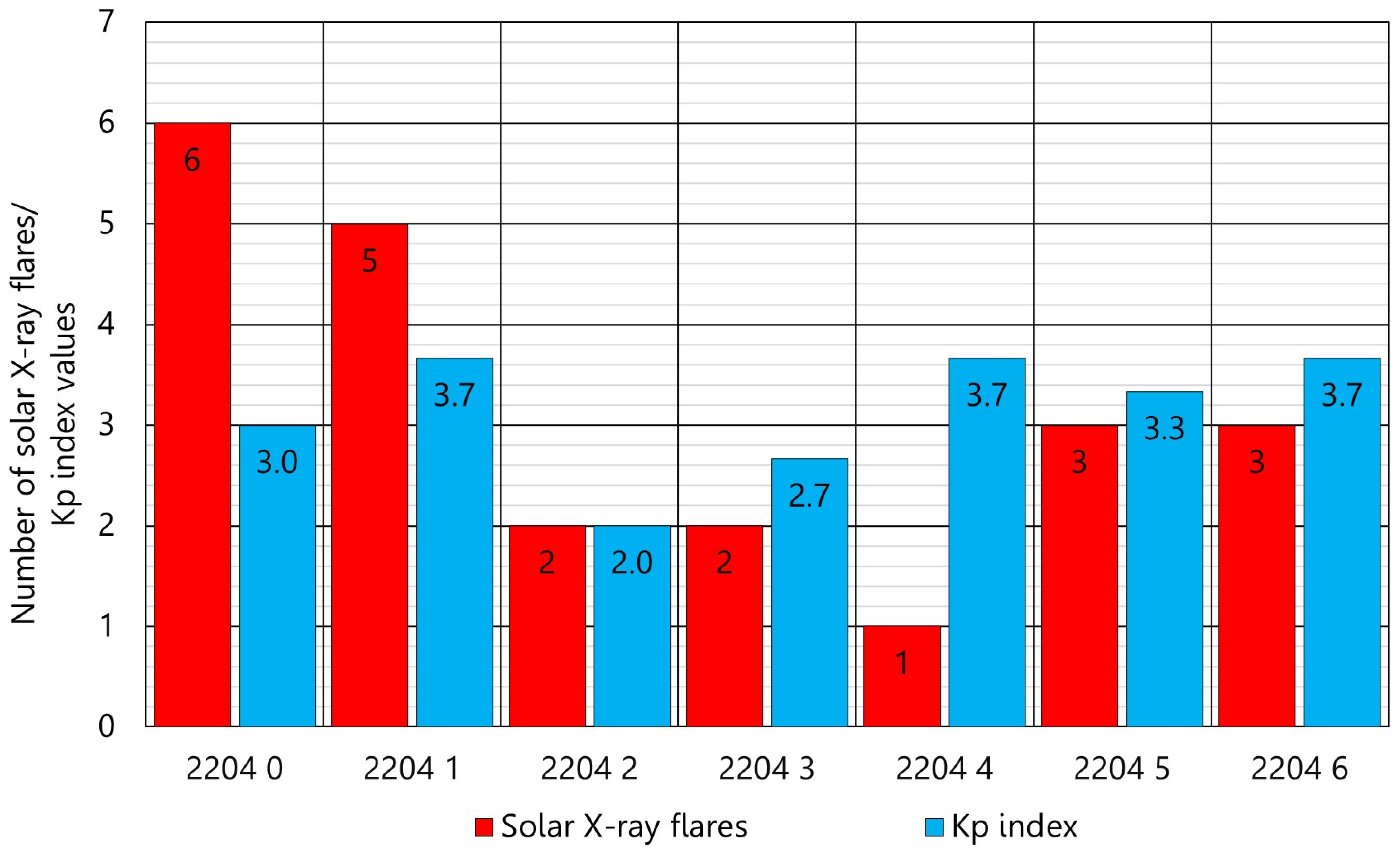
- The D-region exists at lower altitudes (from 50 km to 90 km) only during daytime and exhibits weak ionisation. The influence of the D-region is generally considered negligible. However, during the solar cycle maximum and periods of maximum perturbations of electron concentration caused by solar X flares, the influence is not insignificant [5];
- The E-region (from 90 km to 140 km) represents an intermediate region with moderate ionisation, present both during the day and partially at night. Compared to the higher regions, the E-region is weakly ionised. Although partially present at night, this region has a minor effect on radio waves, compared to higher ones;
- The F-region (from 140 km to 1000 km) contains the highest concentration of electrons and is the most significant for radio wave propagation [6]. During the day, the F-region splits into the F1 and F2 regions. The F2 is the most significant cause of delay in satellite signals and is the most critical for navigation and space communication. A high variability rate also characterises this region in time, so it is difficult to predict its impact. It is present both during the day and during the night [7].
- The direct approach, which utilises existing ionospheric models to minimise their impact on GNSS positioning and support other aspects of data processing;
- The indirect approach, which leverages GNSS observations to estimate ionospheric parameters and develop ionospheric models.
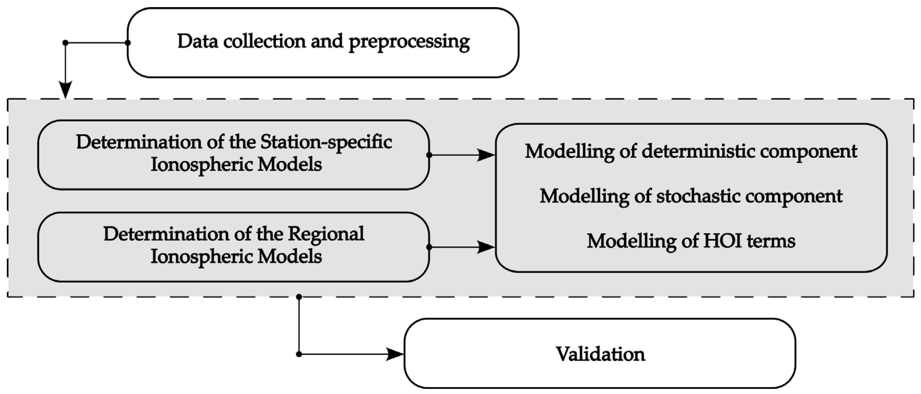
2. Data and Methodology
2.1. Mathematical Background
- Deterministic component;
- Stochastic component.
2.1.1. Deterministic Component
- Local ionospheric models based on two-dimensional Taylor series expansions;
- Global or regional ionospheric models based on spherical harmonic expansion;
- Station-specific ionospheric models, represented as (2), with an estimated set of ionosphere parameters for each station involved.
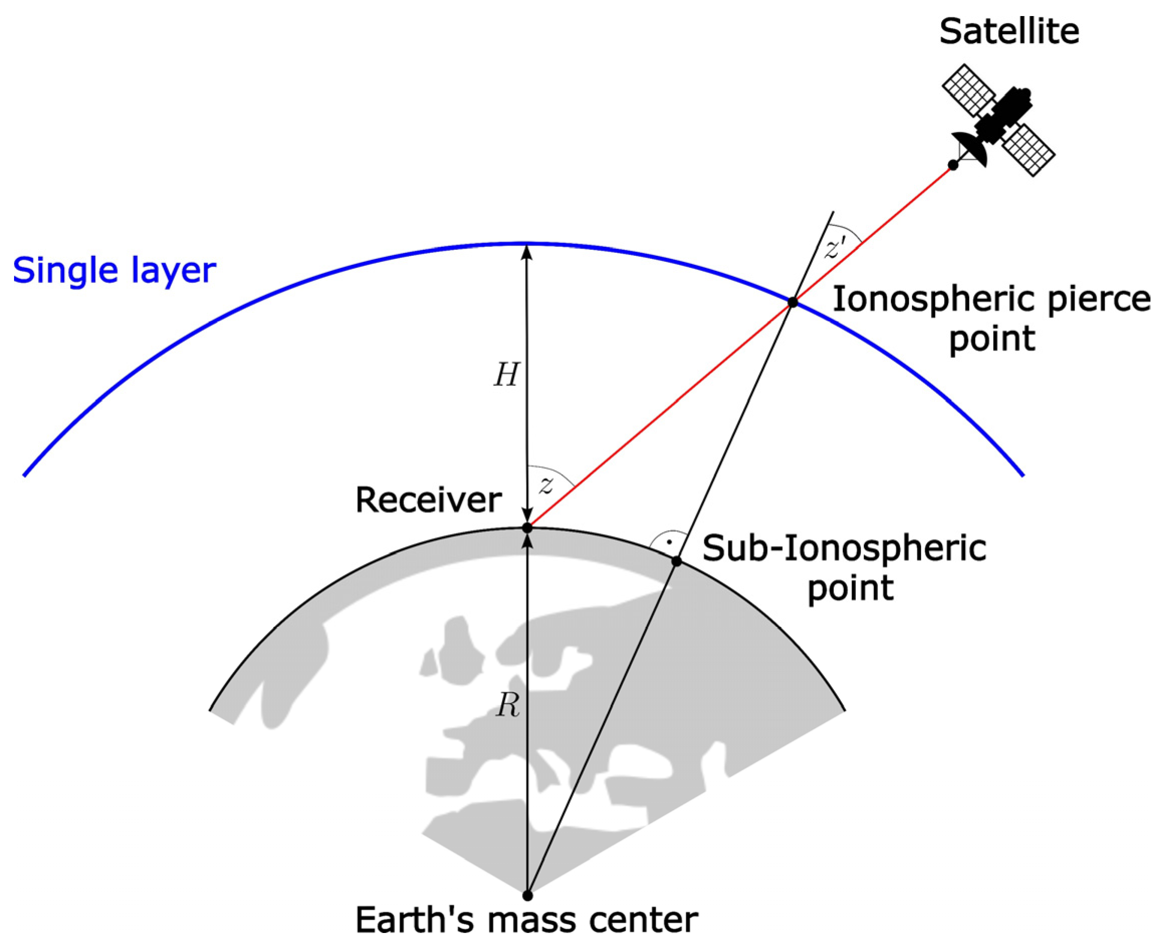
2.1.2. Mapping Function
- It is assumed that the free electrons in the ionosphere are concentrated within a thin membrane (shell) at a constant height above the Earth’s surface;
- The height of the ionospheric shell is adopted following the characteristic profile of the ionosphere;
- The satellite signal emitted by the satellite changes its direction of propagation when interacting with the ionospheric shell;
- The adopted height is considered a fixed value.
2.1.3. Stochastic Component
2.1.4. High-Order Terms and Signal-Bending Effect
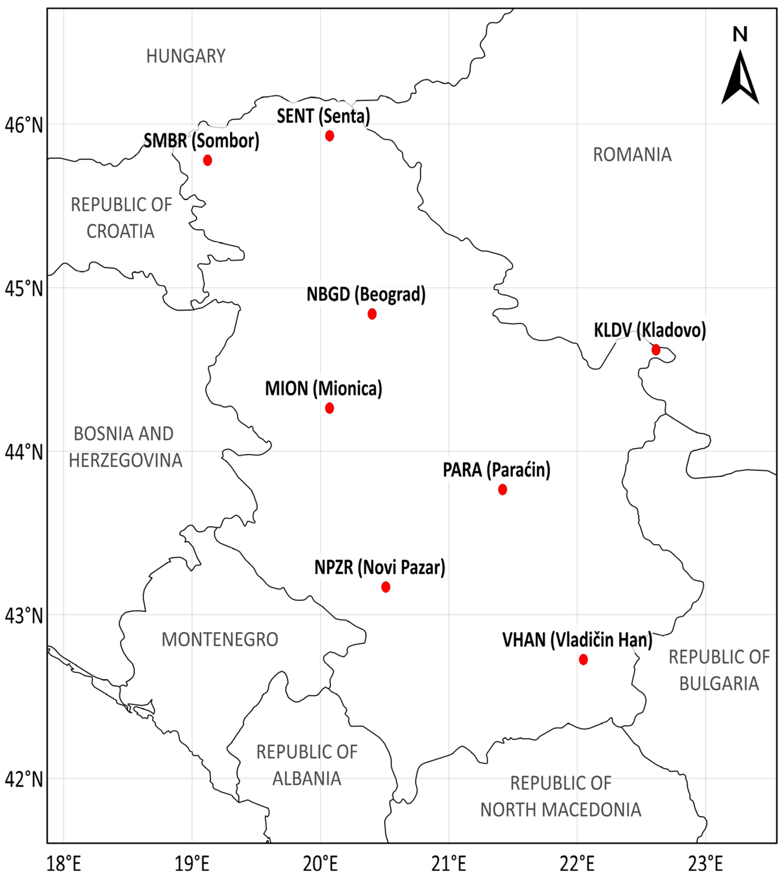
2.2. Study Area and Data Collection
2.3. Software and Computation Strategy
3. Results and Discussion
3.1. Station-Specific (Local) Ionospheric Models
- Ionospheric modelling was performed by modelling the stochastic and deterministic components, considering higher-order ionospheric correction terms;
- Unknown TEC parameters and of the spherical harmonic expansion were estimated for all GNSS stations with the initial values of the maximum degree and order ;
- The height of the ionosphere layer within the single-layer model was chosen as 450 km;
- In terms of the mode of temporal modelling, the ionospheric models represented static (frozen) TEC structures in the sun-fixed frame with reference to specific time intervals;
- This approach assumes that the TEC distribution remains approximately constant within each interval, allowing dynamic changes to be captured by generating successive models over time;
- The MSLM mapping function was chosen for mapping slant TEC values into vertical TEC;
- The solar magnetic (SM) coordinate system was chosen as the reference frame of coordinates ;
- Estimated spherical harmonic coefficients were developed in the ION format and valid for 24 h;
- For each selected GNSS station, an estimate of unknown DCB parameters was also performed.
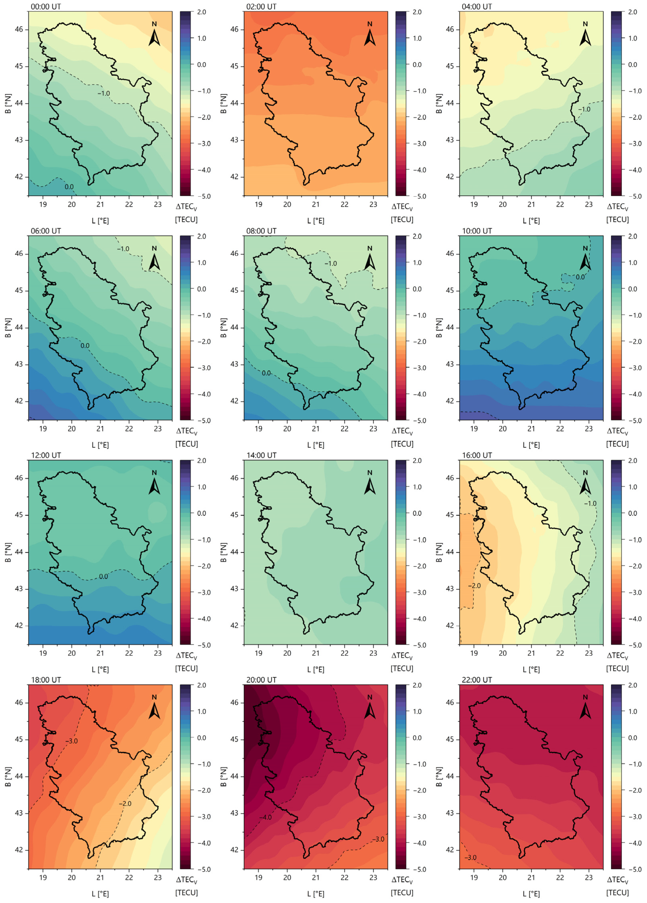
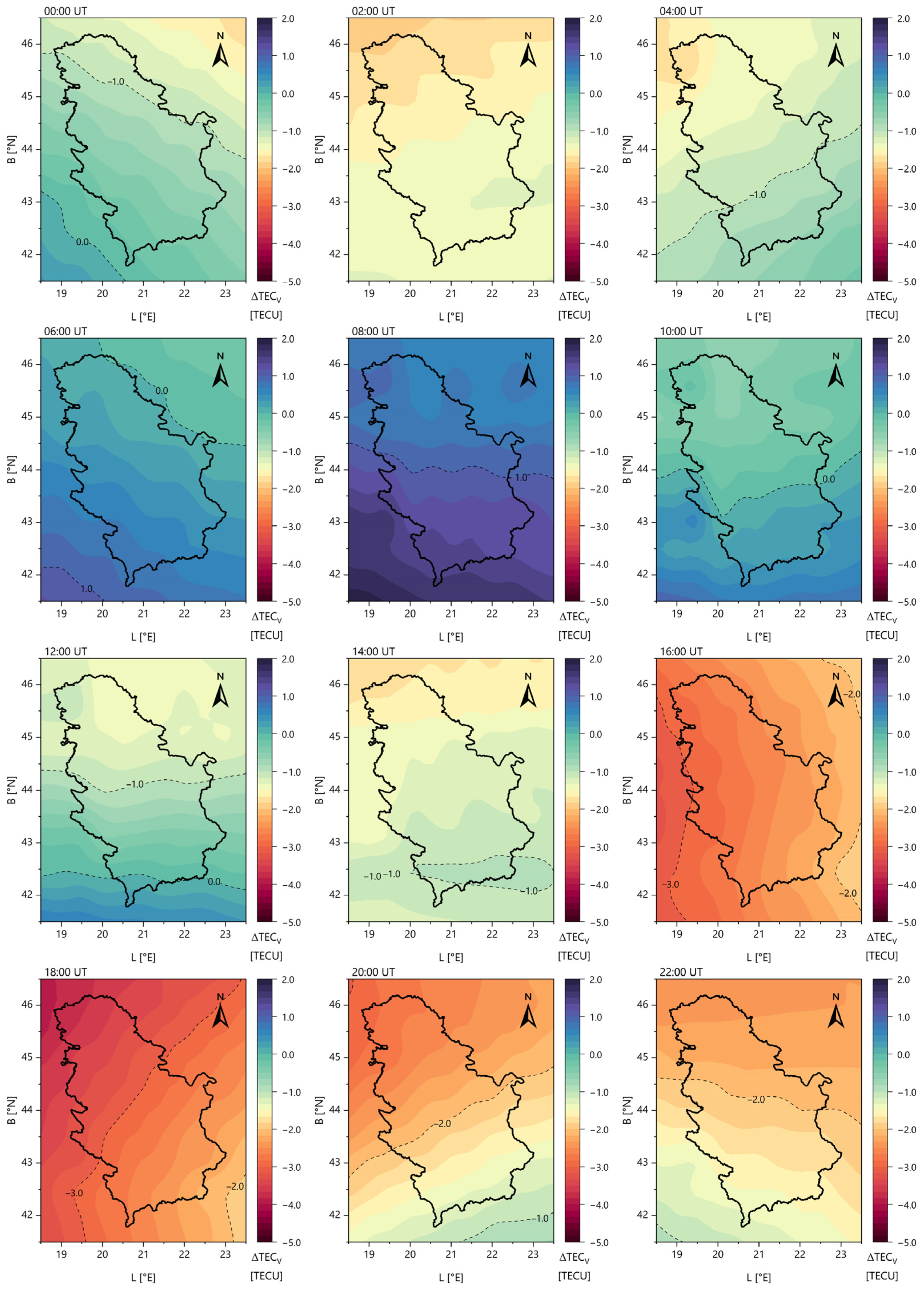
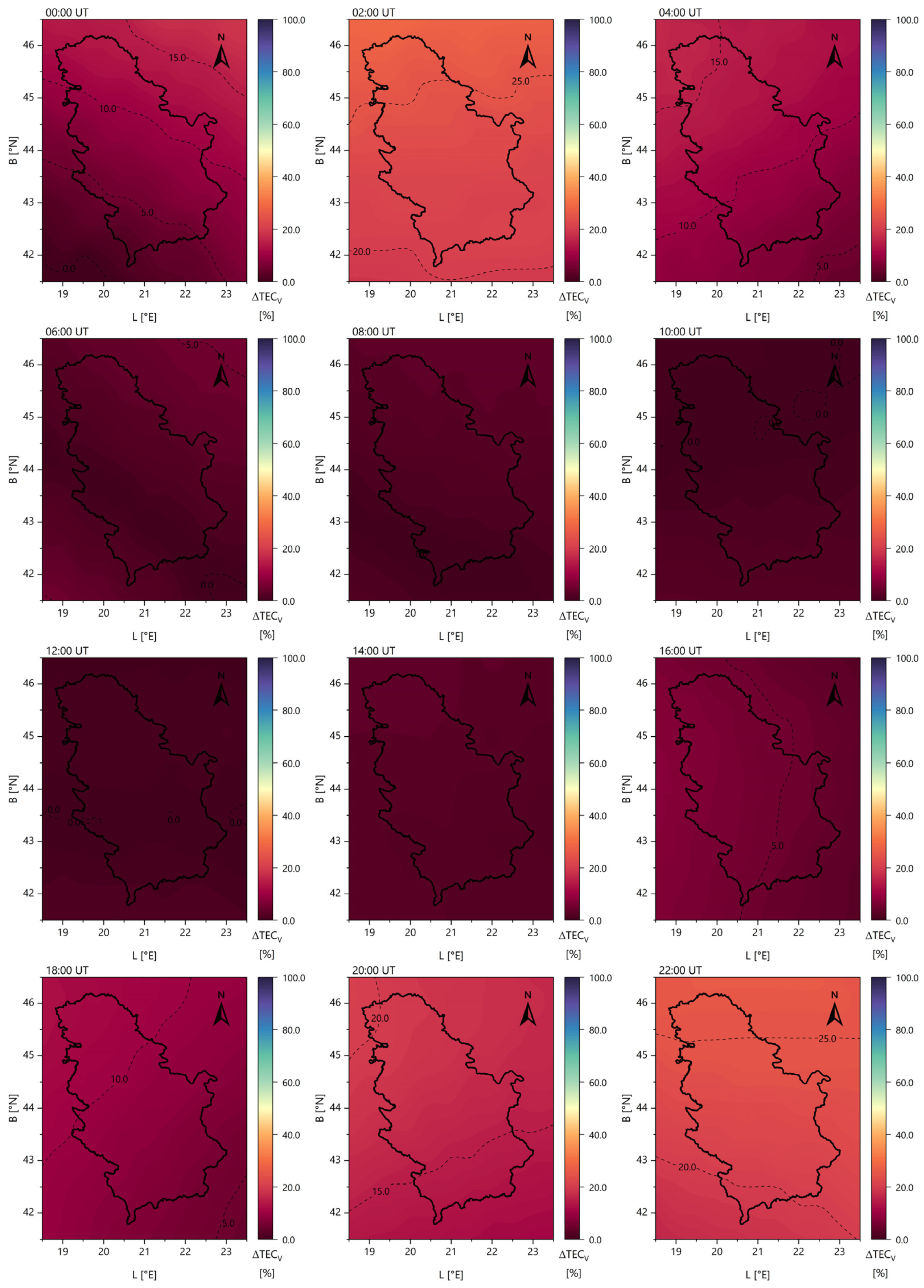
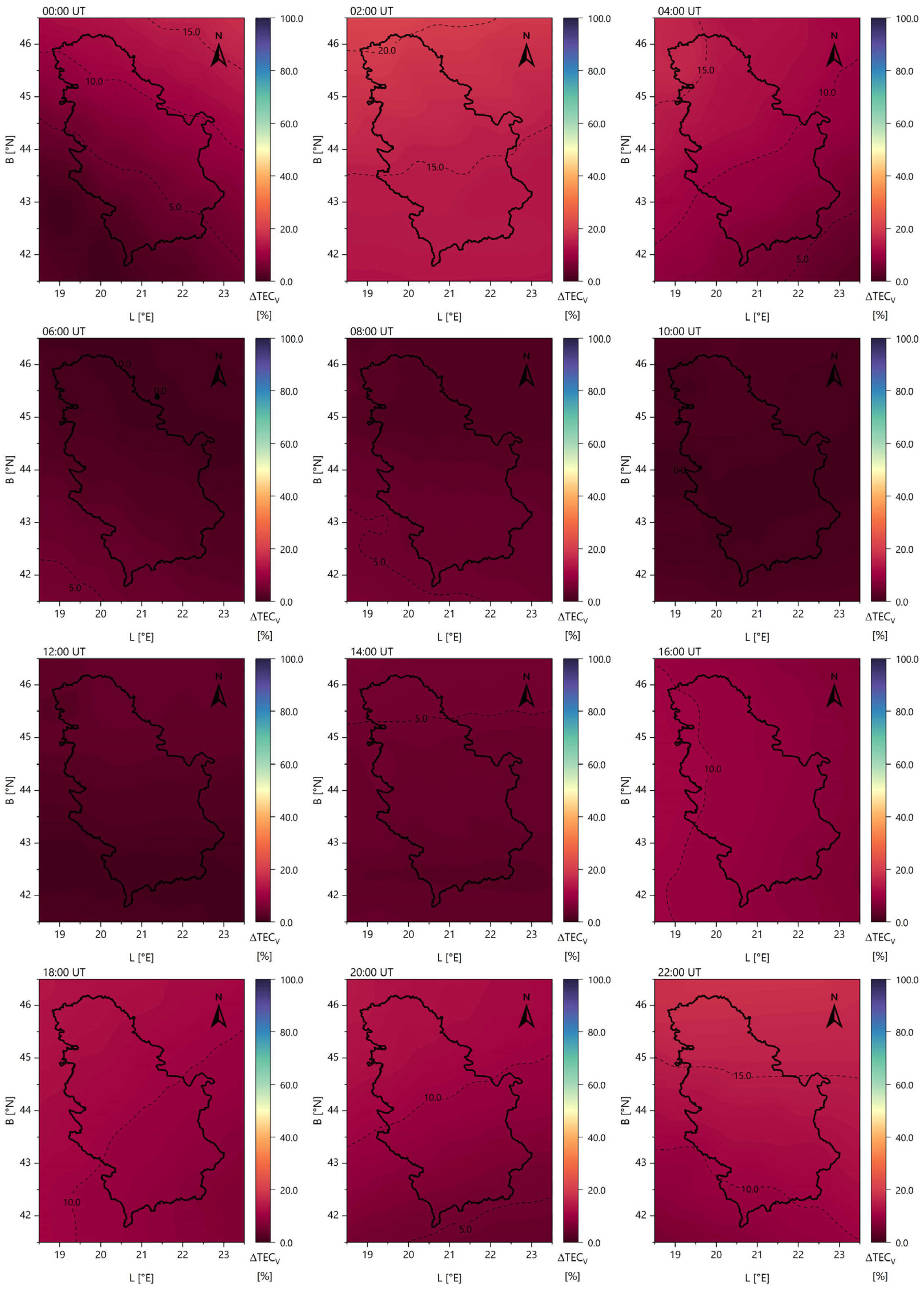
3.2. Regional Ionospheric Models
- The modelling was conducted for the territory of the Republic of Serbia (one set of SH coefficients with the initial values ), covering the latitude range from N to N and the longitude range from E to E;
- The spatial resolution of the created models was ();
- The temporal resolution of the created regional models was 2 h.
- The average RMS value was approximately 0.3 TECU, with most values ranging from 0.2 to 0.5 TECU. These values correspond to the ionospheric maps generated during the deterministic component modelling process.
- The RMS values were nearly two to three times higher when modelling the stochastic component. The specific values depended on the TEC estimates obtained from stochastic modelling, with the RMS values increasing as the TEC values increased. In most cases, the RMS values ranged from 0.6 to 1.2 TECU.
3.3. Ionospheric Modelling Parameters Analysis
3.4. Validation
4. Conclusions
- Modelling the TEC as a harmonic function, i.e., by estimating the SH expansion coefficients, results in local ionospheric models that represent ionospheric conditions more accurately than traditional Taylor series-based approaches.
- High-resolution regional ionospheric models can be developed based on local models, offering a more accurate representation of the ionosphere compared to publicly available GIMs.
- The developed local and regional models incorporate both the deterministic and stochastic components, providing a detailed and precise depiction of ionospheric conditions over the study area within the defined timeframe.
- The agreement between the generated ionospheric models and GIM data was observed within 5 TECU, indicating a significant improvement in regional representation for GNSS data processing.
- The choice of the maximum degree and order in the SH expansion plays a crucial role in the accuracy of the models and should not be overlooked when selecting modelling parameters. It was shown that TEC values do not change significantly with an increase in the maximum degree and order of the SH expansion above eight.
- TEC RMS values primarily depend on the type of the modelled ionospheric component, particularly on the presence of stochastic parameters. While the RMS values ranged from 0.2 to 0.5 TECU for the deterministic components, introducing the stochastic components can increase RMS values by two to three times. It is worth noting that RMS values associated with global ionospheric maps typically span a broader range, with extreme cases reaching values as high as 2 TECU.
Author Contributions
Funding
Institutional Review Board Statement
Informed Consent Statement
Data Availability Statement
Acknowledgments
Conflicts of Interest
Abbreviations
| CODE | Center for Orbit Determination in Europe |
| COSPAR | Committee on Space Research |
| DCB | Differential code bias |
| DGR | Di Giovanni and Radicella |
| DOW | Day of week |
| ESA | European Space Agency |
| GIM | Global ionospheric maps |
| GLONASS | Globalnaya Navigationnaya Sputnikovaya Sistema |
| GNSS | Global navigation satellite system |
| GPS | Global Positioning System |
| HOI | Higher-order ionosphere |
| ICTP | Abdus Salam International Centre for Theoretical Physics |
| IGAM | Institute for Geophysics, Astrophysics, and Meteorology |
| IGS | International GNSS Service |
| IONEX | IONosphere map EXchange |
| IRI | International Reference Ionosphere |
| ITU | International Telecommunication Union |
| LF | Low-frequency |
| MSLM | Modified single-layer model |
| PPP | Precise point positioning |
| RIM | Regional ionospheric models |
| RMS | Root mean square |
| SIP | Stochastic ionospheric parameter |
| SLM | Single-layer model |
| SM | Solar magnetic |
| TID | Travelling ionospheric disturbance |
| URSI | International Union of Radio Science |
| VLF | Very-low-frequency |
| RTK | Real-time kinematic |
| CDDIS | Crustal Dynamics Data Information System |
| RINEX | Receiver Independent Exchange |
| SH | Spherical harmonic |
| IGRF | International geomagnetic reference field |
| TEC | Total electron content |
| TECU | Total electron content unit |
| TECV | Vertical total electron content |
References
- Davies, K. Ionospheric Radio, 3rd ed.; The Institution of Engineering and Technology: London, UK, 1990. [Google Scholar] [CrossRef]
- Schunk, R.; Nagy, A. Ionospheres. Physics, Plasma Physics, and Chemistry, 2nd ed.; Cambridge University Press: New York, NY, USA, 2009. [Google Scholar] [CrossRef]
- Budden, K.B. The Propagation of Radio Waves. The Theory of Radio Waves of Low Power in the Ionosphere and Magnetosphere, 1st ed.; Cambridge University Press: New York, NY, USA, 1985. [Google Scholar] [CrossRef]
- Memarzadeh, Y. Ionospheric Modelling for Precise GNSS Applications. Ph.D. Thesis, Delft University of Technology, Delft, The Netherlands, 2009. [Google Scholar]
- Nina, A.; Nico, G.; Odalović, O.; Čadež, V.M.; Todorović Drakul, M.; Radovanović, M.; Popović, L.Č. GNSS and SAR Signal Delay in Perturbed Ionospheric D-Region During Solar X-Ray Flares. IEEE Geosci. Remote Sens. Lett. 2020, 17, 1198–1202. [Google Scholar] [CrossRef]
- Schaer, S. Mapping and Predicting the Earth’s Ionosphere Using the Global Positioning System. Ph.D. Thesis, Astronomical Institute, University of Bern, Bern, Switzerland, 1999. [Google Scholar]
- Hofmann-Wellenhof, B.; Lichtenegger, H.; Wasle, E. GNSS—Global Navigation Satellite Systems. GPS, GLONASS, Galileo, and More, 1st ed.; SpringerWienNewYork: Vienna, Austria, 2008. [Google Scholar] [CrossRef]
- Seeber, G. Satellite Geodesy. Foundations, Methods, and Applications, 2nd ed.; De Gruyter: Berlin, Germany, 2003. [Google Scholar] [CrossRef]
- Bilitza, D. IRI the International Standard for the Ionosphere. Adv. Radio Sci. 2018, 16, 1–11. [Google Scholar] [CrossRef]
- Radicella, S.M.; Nava, B. Chapter 6—Empirical ionospheric models. In The Dynamical Ionosphere. A Systems Approach to Ionospheric Irregularity, 1st ed.; Materassi, M., Forte, B., Coster, A.J., Skone, S., Eds.; Elsevier: Amsterdam, The Netherlands, 2020; pp. 39–53. [Google Scholar] [CrossRef]
- Bilitza, D. International Reference Ionosphere 2000. Radio Sci. 2001, 36, 261–275. [Google Scholar] [CrossRef]
- Bilitza, D.; Altadill, D.; Zhang, Y.; Mertens, C.; Truhlik, V.; Richards, P.; McKinnell, L.-A.; Reinisch, B. The International Reference Ionosphere 2012—A model of international collaboration. J. Space Weather Space Clim. 2014, 4, A07. [Google Scholar] [CrossRef]
- Bilitza, D.; Altadill, D.; Truhlik, V.; Shubin, V.; Galkin, I.; Reinisch, B.; Huang, X. International Reference Ionosphere 2016: From ionospheric climate to real-time weather predictions. Space Weather 2017, 15, 418–429. [Google Scholar] [CrossRef]
- Bilitza, D.; Pezzopane, M.; Truhlik, V.; Altadill, D.; Reinisch, B.W.; Pignalberi, A. The International Reference Ionosphere model: A review and description of an ionospheric benchmark. Rev. Geophys. 2022, 60, e2022RG000792. [Google Scholar] [CrossRef]
- Di Giovanni, G.; Radicella, S.M. An analytical model of the electron density profile in the ionosphere. Adv. Space Res. 1990, 10, 27–30. [Google Scholar] [CrossRef]
- Nava, B.; Coïsson, P.; Radicella, S.M. A new version of the NeQuick ionosphere electron density model. J. Atmos. Sol.-Terr. Phys. 2008, 70, 1856–1862. [Google Scholar] [CrossRef]
- Nava, B.; Radicella, S.M.; Azpilicueta, F. Data ingestion into NeQuick 2. Radio Sci. 2011, 46, RS0D17. [Google Scholar] [CrossRef]
- Radicella, S.M. The NeQuick model genesis, uses and evolution. Ann. Geophys. 2009, 52, 417–422. [Google Scholar] [CrossRef]
- Subirana, J.S.; Zornoza, J.M.J.; Hernández-Pajares, M. GNSS Data Processing. Volume I: Fundamentals and Algorithms, 1st ed.; TM-23/1; ESA Communications: Noordwijk, The Netherlands, 2013. [Google Scholar]
- Falcone, M.; Hahn, J.; Burger, T. Galileo. In Springer Handbook of Global Navigation Satellite Systems, 1st ed.; Teunissen, P.J.G., Montenbruck, O., Eds.; Springer International Publishing: Cham, Switzerland, 2017; pp. 247–272. [Google Scholar] [CrossRef]
- Semeter, J. Chapter 15—High-resolution approaches to Ionospheric exploration. In The Dynamical Ionosphere. A Systems Approach to Ionospheric Irregularity, 1st ed.; Materassi, M., Forte, B., Coster, A.J., Skone, S., Eds.; Elsevier: Amsterdam, The Netherlands, 2020; pp. 223–241. [Google Scholar] [CrossRef]
- Bibl, K.; Reinisch, B.W. The universal digital ionosonde. Radio Sci. 1978, 13, 519–530. [Google Scholar] [CrossRef]
- Reinisch, B.W.; Galkin, I.A.; Khmyrov, G.M.; Kozlov, A.V.; Bibl, K.; Lisysyan, I.A.; Cheney, G.P.; Huang, X.; Kitrosser, D.F.; Paznukhov, V.V.; et al. New Digisonde for research and monitoring applications. Radio Sci. 2009, 44, RS0A24. [Google Scholar] [CrossRef]
- Mošna, Z.; Kouba, D.; Knížová, P.K.; Burešová, D.; Chum, J.; Šindelářová, T.; Urbář, J.; Boška, J.; Saxonbergová-Jankovičová, D. Ionospheric storm of September 2017 observed at ionospheric station Pruhonice, the Czech Republic. Adv. Space Res. 2020, 65, 115–128. [Google Scholar] [CrossRef]
- Wang, J.; Chen, G.; Yu, T.; Deng, Z.; Yan, X.; Yang, N. Middle-Scale Ionospheric Disturbances Observed by the Oblique-Incidence Ionosonde Detection Network in North China after the 2011 Tohoku Tsunamigenic Earthquake. Sensors 2021, 21, 1000. [Google Scholar] [CrossRef]
- Nina, A.; Nico, G.; Mitrović, S.T.; Čadež, V.M.; Milošević, I.R.; Radovanović, M.; Popović, L.Č. Quiet Ionospheric D-Region (QIonDR) Model Based on VLF/LF Observations. Remote Sens. 2021, 13, 483. [Google Scholar] [CrossRef]
- Nina, A. Modelling of the Electron Density and Total Electron Content in the Quiet and Solar X-ray Flare Perturbed Ionospheric D-Region Based on Remote Sensing by VLF/LF Signals. Remote Sens. 2022, 14, 54. [Google Scholar] [CrossRef]
- Pal, S.; Hobara, Y.; Shvets, A.; Schnoor, P.W.; Hayakawa, M.; Koloskov, O. First Detection of Global Ionospheric Disturbances Associated with the Most Powerful Gamma Ray Burst GRB221009A. Atmosphere 2023, 14, 217. [Google Scholar] [CrossRef]
- Langley, R.B.; Teunissen, P.J.; Montenbruck, O. Introduction to GNSS. In Springer Handbook of Global Navigation Satellite Systems, 1st ed.; Teunissen, P.J.G., Montenbruck, O., Eds.; Springer International Publishing: Cham, Switzerland, 2017; pp. 3–23. [Google Scholar] [CrossRef]
- Dach, R.; Lutz, S.; Walser, P.; Fridez, P. Bernese GNSS Software, Version 5.2; User Manual; University of Bern, Bern Open Publishing: Bern, Switzerland, 2015. [CrossRef]
- Klobuchar, J.A. Ionospheric Time-Delay Algorithm for Single-Frequency GPS Users. IEEE Trans. Aerosp. Electron. Syst. 1987, AES-23, 325–331. [Google Scholar] [CrossRef]
- Wild, U. Ionosphere and Geodetic Satellite Systems: Permanent GPS Tracking Data for Modelling and Monitoring. Ph.D. Thesis, Swiss Geodetic Commission, ETH Zurich, Zurich, Switzerland, 1994. [Google Scholar]
- Komjathy, A. Global Ionospheric Total Electron Content Mapping Using the Global Positioning System. Ph.D. Thesis, Department of Geodesy and Geomatics Engineering Technical Report No. 188, University of New Brunswick, Fredericton, NB, Canada, 1997. [Google Scholar]
- Schaer, S.; Beutler, G.; Mervart, L.; Rothacher, M.; Wild, U. Global and regional ionosphere models using the GPS double difference phase observable. In Proceedings of the IGS Workshop, Potsdam, Germany, 15–17 May 1995. [Google Scholar]
- Schaer, S.; Beutler, G.; Rothacher, M. Mapping and predicting the ionosphere. In Proceedings of the IGS AC Workshop, Darmstadt, Germany, 9–11 February 1998. [Google Scholar]
- Hernández-Pajares, M.; Juan, J.M.; Sanz, J.; Orus, R.; Garcia-Rigo, A.; Feltens, J.; Komjathy, A.; Schaer, S.C.; Krankowski, A. The IGS VTEC maps: A reliable source of ionospheric information since 1998. J. Geod. 2009, 83, 263–275. [Google Scholar] [CrossRef]
- International GNSS Service. Available online: https://igs.org/ (accessed on 17 March 2025).
- Hernández-Pajares, M.; Roma-Dollase, D.; Krankowski, A.; García-Rigo, A.; Orús-Pérez, R. Methodology and consistency of slant and vertical assessments for ionospheric electron content models. J. Geod. 2017, 91, 1405–1414. [Google Scholar] [CrossRef]
- Roma-Dollase, D.; Hernández-Pajares, M.; Krankowski, A.; Kotulak, K.; Ghoddousi-Fard, R.; Yuan, Y.; Li, Z.; Zhang, H.; Shi, C.; Wang, C.; et al. Consistency of seven different GNSS global ionospheric mapping techniques during one solar cycle. J. Geod. 2017, 92, 691–706. [Google Scholar] [CrossRef]
- Li, Z.; Wang, N.; Hernández-Pajares, M.; Yuan, Y.; Krankowski, A.; Liu, A.; Zha, J.; García-Rigo, A.; Roma-Dollase, D.; Yang, H.; et al. IGS real-time service for global ionospheric total electron content modelling. J. Geod. 2020, 94, 32. [Google Scholar] [CrossRef]
- Cherniak, I.; Krankowski, A.; Zakharenkova, I. Observation of the ionospheric irregularities over the Northern Hemisphere: Methodology and service. Radio Sci. 2014, 49, 653–662. [Google Scholar] [CrossRef]
- Galkin, I.; Froń, A.; Reinisch, B.; Hernández-Pajares, M.; Krankowski, A.; Nava, B.; Bilitza, D.; Kotulak, K.; Flisek, P.; Li, Z.; et al. Global Monitoring of Ionospheric Weather by GIRO and GNSS Data Fusion. Atmosphere 2022, 13, 371. [Google Scholar] [CrossRef]
- Todorović Drakul, M. Ionosphere Modelling for the Purposes of Determination of Influence to the GPS Signals Within Network RTK Environment. Ph.D. Thesis, University of Belgrade, Faculty of Civil Engineering, Belgrade, Serbia, 2016. [Google Scholar]
- Todorović Drakul, M.; Čadez, V.; Bajčetić, J.; Popović, L.; Blagojević, D.; Nina, A. Behaviour of electron content in the ionospheric D-region during solar X-ray flares. Serbian Astron. J. 2016, 193, 11–18. [Google Scholar] [CrossRef]
- Todorović Drakul, M.; Samardžić-Petrović, M.; Grekulović, S.; Odalović, O.; Blagojević, D. Modelling extreme values of the total electron content: Case study of Serbia. Geofizika 2017, 34, 297–314. [Google Scholar] [CrossRef]
- Natras, R.; Goss, A.; Halilovic, D.; Magnet, N.; Mulic, M.; Schmidt, M.; Weber, R. Regional Ionosphere Delay Models Based on CORS Data and Machine Learning. Navig. J. Inst. Navig. 2023, 70, navi.577. [Google Scholar] [CrossRef]
- Schaer, S.; Gurtner, W.; Feltens, J. IONEX: The IONosphere Map Exchange Format Version 1.0. In Proceedings of the IGS AC Workshop, Darmstadt, Germany, 9–11 February 1998. [Google Scholar]
- Schaer, S.; Gurtner, W.; Feltens, J. IONEX: The IONosphere Map Exchange Format Version 1.1. In Proceedings of the IGS AC Workshop, Darmstadt, Germany, 9–11 February 1998. [Google Scholar]
- Padokhin, A.M.; Andreeva, E.S.; Nazarenko, M.O.; Kalashnikova, S.A. Phase-Difference Approach for GNSS Global Ionospheric Total Electron Content Mapping. Radiophys. Quantum Electron. 2022, 65, 481–495. [Google Scholar] [CrossRef]
- Ren, X.; Zhang, X.; Xie, W.; Zhang, K.; Yuan, Y.; Li, X. Global Ionospheric Modelling Using Multi-GNSS: BeiDou, Galileo, and GPS. Sci. Rep. 2016, 6, 33499. [Google Scholar] [CrossRef]
- Zhang, Q.; Zhao, Q. Analysis of the Data Processing Strategies of Spherical Harmonic Expansion Model on Global Ionosphere Mapping for Moderate Solar Activity. Adv. Space Res. 2019, 63, 1214–1226. [Google Scholar] [CrossRef]
- Choi, B.-K.; Lee, W.K.; Cho, S.-K.; Park, J.-U.; Park, P.-H. Global GPS Ionospheric Modelling Using Spherical Harmonic Expansion Approach. J. Astron. Space Sci. 2010, 27, 359–366. [Google Scholar] [CrossRef]
- Mehmood, M.; Shahid, I.; Nawaz, R.; Mushtaq, S. Total Electron Content (TEC) Estimation over Pakistan from Local GPS Network. Ann. Geophys. 2021, 64, GD102. [Google Scholar] [CrossRef]
- Liu, J.; Chen, R.; An, J.; Hyyppa, J. Spherical Cap Harmonic Analysis of the Arctic Ionospheric TEC for One Solar Cycle. J. Geophys. Res. Space Phys. 2014, 119, 601–619. [Google Scholar] [CrossRef]
- Li, W.; Zhao, D.; Shen, Y.; Zhang, K. Modeling Australian TEC Maps Using Long-Term Observations of Australian Regional GPS Network by Artificial Neural Network-Aided Spherical Cap Harmonic Analysis Approach. Remote Sens. 2020, 12, 3851. [Google Scholar] [CrossRef]
- Liu, J.; Chen, R.; Wang, Z.; Zhang, H. Spherical Cap Harmonic Model for Mapping and Predicting Regional TEC. GPS Solut. 2011, 15, 109–119. [Google Scholar] [CrossRef]
- Hauschild, A. Basic Observation Equations. In Springer Handbook of Global Navigation Satellite Systems, 1st ed.; Teunissen, P.J.G., Montenbruck, O., Eds.; Springer International Publishing: Cham, Switzerland, 2017; pp. 561–582. [Google Scholar] [CrossRef]
- Jakowski, N. Ionosphere Monitoring. In Springer Handbook of Global Navigation Satellite Systems, 1st ed.; Teunissen, P.J.G., Montenbruck, O., Eds.; Springer International Publishing: Cham, Switzerland, 2017; pp. 1139–1162. [Google Scholar] [CrossRef]
- Hobiger, T.; Jakowski, N. Atmospheric Signal Propagation. In Springer Handbook of Global Navigation Satellite Systems, 1st ed.; Teunissen, P.J.G., Montenbruck, O., Eds.; Springer International Publishing: Cham, Switzerland, 2017; pp. 165–193. [Google Scholar] [CrossRef]
- Seemala, G.K. Chapter 4—Estimation of ionospheric total electron content (TEC) from GNSS observations. In Atmospheric Remote Sensing: Principles and Applications, 1st ed.; Singh, A.K., Tiwari, S., Eds.; Elsevier: Amsterdam, The Netherlands, 2023; pp. 63–84. [Google Scholar] [CrossRef]
- Böhm, J.; Schuh, H. Atmospheric Effects in Space Geodesy, 1st ed.; Springer: Berlin/Heidelberg, Germany, 2013. [Google Scholar] [CrossRef]
- Odalović, O.; Petković, D.; Grekulović, S.; Todorović Drakul, M. A compliance assessment of GNSS station networks in Serbia. J. Geogr. Inst. Jovan Cvijić SASA 2024, 74, 47–61. [Google Scholar] [CrossRef]
- Space Weather Prediction Center, National Oceanic and Atmospheric Administration. Available online: https://www.swpc.noaa.gov/noaa-scales-explanation (accessed on 11 January 2024).
- Space Weather. Available online: https://www.spaceweatherlive.com/en/archive.html (accessed on 4 August 2023).
- The Helmholtz Centre Potsdam—GFZ German Research Centre for Geosciences. Available online: https://kp.gfz-potsdam.de/en/ (accessed on 25 December 2023).
- Dach, R.; Schaer, S.; Arnold, D.; Brockmann, E.; Kalarus, M.S.; Lasser, M.; Stebler, P.; Jäggi, A. CODE Final Product Series for the IGS; Astronomical Institute, University of Bern: Bern, Switzerland, 2024; Available online: https://www.aiub.unibe.ch/download/CODE (accessed on 17 July 2023). [CrossRef]
- Johnston, G.; Riddell, A.; Hausler, G. The International GNSS Service. In Springer Handbook of Global Navigation Satellite Systems, 1st ed.; Teunissen, P.J.G., Montenbruck, O., Eds.; Springer International Publishing: Cham, Switzerland, 2017; pp. 967–982. [Google Scholar] [CrossRef]
- Noll, C. The Crustal Dynamics Data Information System: A resource to support scientific analysis using space geodesy. Adv. Space Res. 2010, 45, 1421–1440. [Google Scholar] [CrossRef]
- Dach, R.; Fridez, P. Bernese GNSS Software, Version 5.2; Tutorial; University of Bern, Bern Open Publishing: Bern, Switzerland, 2021.
- Dach, R.; Arnold, D. Bernese GNSS Software, Version 5.4; Tutorial; University of Bern, Bern Open Publishing: Bern, Switzerland, 2025.
- Alken, P.; Thébault, E.; Beggan, C.D.; Amit, H.; Aubert, J.; Baerenzung, J.; Bondar, T.N.; Brown, W.J.; Califf, S.; Chambodut, A.; et al. International Geomagnetic Reference Field: The thirteenth generation. Earth Planets Space 2021, 73, 49. [Google Scholar] [CrossRef]
- Laundal, K.M.; Richmond, A.D. Magnetic Coordinate Systems. Space Sci. Rev. 2017, 206, 27–59. [Google Scholar] [CrossRef]
- Hapgood, M.A. Space physics coordinate transformations: A user guide. Planet. Space Sci. 1992, 40, 711–717. [Google Scholar] [CrossRef]
- Russell, C.T. Geophysical Coordinate Transformations. Cosm. Electrodyn. 1971, 2, 184–196. [Google Scholar]
- Crustal Dynamics Data Information System (CDDIS DAAC). Available online: https://cddis.nasa.gov/archive/gnss/products/ionex/ (accessed on 17 July 2023).


| Station ID | Location | Receiver/ Antenna | |||
|---|---|---|---|---|---|
| Town Name | Latitude B [°N] | Longitude L [°E] | Ellipsoidal Height h [m] | ||
| KLDV | Kladovo | 44.60901 | 22.63690 | 97.24 | ComNav M300 Mini/ComNav AT330 (GPS, GLONASS, BeiDou, Galileo) |
| MION | Mionica | 44.25117 | 20.08014 | 237.43 | |
| NBGD | Beograd | 44.82887 | 20.41289 | 140.56 | |
| NPZR | Novi Pazar | 43.15391 | 20.52042 | 572.39 | |
| PARA | Paraćin | 43.75226 | 21.43569 | 189.34 | |
| SMBR | Sombor | 45.77159 | 19.12456 | 149.00 | |
| VHAN | Vladičin Han | 42.70896 | 22.06835 | 388.75 | |
| Date | Statistical Indicator | Station ID | Serbia Average | ||||||
|---|---|---|---|---|---|---|---|---|---|
| KLDV | MION | NBGD | NPZR | PARA | SMBR | VHAN | |||
| 3 April 2022 | MIN | 9.3 | 8.8 | 9.4 | 9.6 | 9.4 | 8.1 | 10.5 | 9.3 |
| MAX | 30.2 | 31.5 | 31.2 | 33.7 | 31.6 | 29.6 | 35.6 | 31.9 | |
| RANGE | 20.9 | 22.7 | 21.8 | 24.1 | 22.2 | 21.5 | 25.1 | 22.6 | |
| 4 April 2022 | MIN | 10.0 | 10.6 | 10.1 | 9.7 | 10.5 | 10.2 | 10.5 | 10.2 |
| MAX | 26.5 | 27.8 | 28.0 | 28.5 | 26.7 | 26.9 | 31.3 | 28.0 | |
| RANGE | 16.5 | 17.2 | 17.9 | 18.8 | 16.2 | 16.7 | 20.8 | 17.7 | |
| 5 April 2022 | MIN | 10.1 | 10.1 | 11.7 | 8.6 | 11.3 | 9.3 | 10.1 | 10.2 |
| MAX | 35.2 | 34.6 | 34.8 | 37.6 | 35.2 | 33.1 | 39.3 | 35.7 | |
| RANGE | 25.2 | 24.6 | 23.1 | 29.0 | 23.9 | 23.9 | 29.2 | 25.5 | |
| 6 April 2022 | MIN | 10.6 | 10.8 | 9.6 | 8.6 | 11.7 | 10.1 | 11.0 | 10.3 |
| MAX | 35.8 | 37.0 | 36.6 | 38.4 | 35.9 | 34.5 | 39.6 | 36.8 | |
| RANGE | 25.2 | 26.3 | 27.0 | 29.8 | 24.3 | 24.4 | 28.6 | 26.5 | |
| 7 April 2022 | MIN | 9.5 | 10.2 | 9.9 | 9.5 | 10.0 | 9.3 | 7.4 | 9.4 |
| MAX | 37.9 | 38.1 | 38.4 | 40.9 | 38.7 | 36.8 | 41.5 | 38.9 | |
| RANGE | 28.4 | 27.9 | 28.5 | 31.5 | 28.7 | 27.4 | 34.1 | 29.5 | |
| 8 April 2022 | MIN | 10.5 | 9.0 | 8.5 | 8.4 | 10.5 | 9.5 | 9.4 | 9.4 |
| MAX | 28.9 | 28.0 | 29.1 | 31.0 | 28.8 | 27.1 | 31.6 | 29.2 | |
| RANGE | 18.4 | 19.0 | 20.6 | 22.6 | 18.3 | 17.5 | 22.2 | 19.8 | |
| 9 April 2022 | MIN | 8.0 | 7.8 | 6.9 | 7.1 | 8.6 | 6.4 | 8.2 | 7.6 |
| MAX | 40.7 | 42.3 | 40.3 | 43.9 | 41.6 | 39.1 | 45.5 | 41.9 | |
| RANGE | 32.7 | 34.5 | 33.4 | 36.8 | 33.0 | 32.7 | 37.2 | 34.3 | |
| Solution ID | |||||||
|---|---|---|---|---|---|---|---|
| MIN | MAX | RANGE | AVG | STDEV | |||
| 1 | 2 | 9 | −1.2 | 5.8 | 7.0 | 1.6 | 1.8 |
| 2 | 3 | 16 | −1.2 | 2.8 | 4.0 | 0.6 | 1.2 |
| 3 | 4 | 25 | −0.4 | 1.6 | 2.0 | 0.4 | 0.6 |
| 4 | 5 | 36 | 0.0 | 1.0 | 1.0 | 0.4 | 0.3 |
| 5 | 6 | 49 | 0.1 | 1.0 | 0.9 | 0.5 | 0.2 |
| 6 | 8 | 81 | - | - | - | - | - |
| 7 | 10 | 121 | −0.2 | 0.4 | 0.6 | 0.1 | 0.1 |
| 8 | 12 | 169 | −0.2 | 0.4 | 0.6 | 0.1 | 0.2 |
| 9 | 14 | 225 | −0.3 | 0.5 | 0.9 | 0.1 | 0.2 |
| 10 | 16 | 289 | −0.5 | 0.5 | 1.0 | 0.0 | 0.3 |
| Statistical Indicator | 2204 6 | |||||||||||
|---|---|---|---|---|---|---|---|---|---|---|---|---|
| 00 | 02 | 04 | 06 | 08 | 10 | 12 | 14 | 16 | 18 | 20 | 22 | |
| MIN | −1.9 | −3.0 | −1.7 | −1.3 | −1.1 | −0.3 | −0.4 | −1.0 | −2.3 | −3.6 | −5.0 * | −3.9 |
| MAX | 0.1 | −2.1 | −0.6 | 1.0 | 0.5 | 0.9 | 0.5 | −0.6 | −0.5 | −1.4 | −2.9 | −2.9 |
| RANGE | 2.0 | 0.9 | 1.1 | 2.3 *** | 1.6 | 1.2 | 0.9 | 0.4 | 1.8 | 2.2 | 2.1 | 1.0 |
| MIN | −1.8 | −2.1 | −1.8 | −0.4 | 0.6 | −0.6 | −1.5 | −1.8 | −3.3 | −4.0 | −3.1 | −2.5 |
| MAX | 0.3 | −1.3 | −0.4 | 1.1 | 1.8 ** | 0.6 | 0.3 | −0.9 | −1.8 | −2.0 | −1.0 | −1.0 |
| RANGE | 2.1 | 0.8 | 1.4 | 1.5 | 1.3 | 1.3 | 1.8 | 0.9 | 1.6 | 2.0 | 2.1 | 1.5 |
Disclaimer/Publisher’s Note: The statements, opinions and data contained in all publications are solely those of the individual author(s) and contributor(s) and not of MDPI and/or the editor(s). MDPI and/or the editor(s) disclaim responsibility for any injury to people or property resulting from any ideas, methods, instructions or products referred to in the content. |
© 2025 by the authors. Licensee MDPI, Basel, Switzerland. This article is an open access article distributed under the terms and conditions of the Creative Commons Attribution (CC BY) license (https://creativecommons.org/licenses/by/4.0/).
Share and Cite
Petković, D.; Odalović, O.; Nina, A.; Todorović-Drakul, M.; Kolarski, A.; Grekulović, S.; Krstić, S. Development of High-Precision Local and Regional Ionospheric Models Based on Spherical Harmonic Expansion and Global Navigation Satellite System Data in Serbia. Atmosphere 2025, 16, 496. https://doi.org/10.3390/atmos16050496
Petković D, Odalović O, Nina A, Todorović-Drakul M, Kolarski A, Grekulović S, Krstić S. Development of High-Precision Local and Regional Ionospheric Models Based on Spherical Harmonic Expansion and Global Navigation Satellite System Data in Serbia. Atmosphere. 2025; 16(5):496. https://doi.org/10.3390/atmos16050496
Chicago/Turabian StylePetković, Dušan, Oleg Odalović, Aleksandra Nina, Miljana Todorović-Drakul, Aleksandra Kolarski, Sanja Grekulović, and Stefan Krstić. 2025. "Development of High-Precision Local and Regional Ionospheric Models Based on Spherical Harmonic Expansion and Global Navigation Satellite System Data in Serbia" Atmosphere 16, no. 5: 496. https://doi.org/10.3390/atmos16050496
APA StylePetković, D., Odalović, O., Nina, A., Todorović-Drakul, M., Kolarski, A., Grekulović, S., & Krstić, S. (2025). Development of High-Precision Local and Regional Ionospheric Models Based on Spherical Harmonic Expansion and Global Navigation Satellite System Data in Serbia. Atmosphere, 16(5), 496. https://doi.org/10.3390/atmos16050496